Phase space contraction and quantum operations

Abstract

We give a criterion to differentiate between dissipative and diffusive quantum operations. It is based on the classical idea that dissipative processes contract volumes in phase space. We define a quantity that can be regarded as “quantum phase space contraction rate” and which is related to a fundamental property of quantum channels: non-unitality. We relate it to other properties of the channel and also show a simple example of dissipative noise composed with a chaotic map. The emergence of attaractor-like structures is displayed.

I Introduction

Quantum dissipative processes in the context of quantum optics Gardiner and Zoller (2000), of superradiance Haake (1992), of cooling mechanisms in ion traps Gardiner et al. (1997) and open nanostructures Mahler and Weberruß (1992) have been widely studied using a master equation approach. The corresponding master equation for each case is derived by modeling a microscopic interaction between the system (according to the case: an oscillator, a large spin, etc.) and a heat bath representing the environment. Under standard approximations (e.g. Born-Markov, random wave)Gardiner and Zoller (2000) one ends with a Lindblad master equation, which automatically insures the preservation of positivity Lindblad (1976); Gorini et al. (1976). For general dissipative processes the operators in the master equation are not normal.

In this article dissipation is understood in analogy with classical dynamics, that is, we call dissipative any process in which phase space volume is not preserved. We have to keep in mind that this definition is different from the concept of ‘dissipativity’ which is often found in the literature. For example, in Lindblad (1976) Lindblad calls dissipative maps the generators of completely positive semigroups, that is, dissipativity is linked to irreversibility. For Lidar et al.Lidar et al. the condition of dissipativity is related to strictly purity decreasing, and shows its close relation to unitality. The concept of phase space contraction is well defined in a classical context as the divergence of the velocity field. In quantum mechanics this divergence can be related to the sum of the commutators of the Lindblad generators in the classical limit. Percival (1998)

The evolution of the density matrix of the system between two given times, that is, the transformation that takes $\rho(t)$ to $\rho(t+\delta t)$ can be obtained by integration of the master equation. This leads to a superoperator which can be written in an operator sum or Kraus form Kraus (1983). The detailed procedure depends on each particular process and can be mathematically complicated. In this work we follow an alternative approach to the description of dissipative quantum noise which consists in directly modeling the superoperator in its Kraus representation. The formalism of quantum operations to describe open systems, which is especially well adapted in the context of quantum information and quantum computing Chuang and Nielsen (2001); Preskill (1998), has also been used for open quantum maps Bianucci et al. (2002); García-Mata et al. (2003); García-Mata and Saraceno (2004); Aolita et al. (2004); Łoziński et al. (2002); Nonnenmacher (2003), which are quantum maps in the usual sense with some non-unitary noise that can be considered the effect of an interaction with some environment.

In Aolita et al. (2004) the authors analyze several models for purely diffusive noises and show that generalization of simple channels known in quantum information theory (depolarizing and phase damping channels) can be written as an incoherent sum of translations in phase space. Since the translation operators are unitary the preservation of the trace implies that the noise superoperator is unital (i.e. identity preserving). In this paper we focus on non-unital channels in a finite dimensional Hilbert space and show that their action can be interpreted as a contraction of the phase space volume leading to dissipative dynamics.

This paper is organized as follows. In Sec. II we briefly go through the formalism of the Lindblad master equation and the superoperator approach. A parameter measuring phase space contraction in the quantum operations formalism is introduced in Sec. III. Some examples of quantum diffusive and dissipative processes are given inSec. IV. In Sec. V we give a simple dissipative channel as an example and show the effects when composed with a unitary map in Sec. VI.

II Master equation and Quantum dynamical semigroups

Open systems involve non-unitary evolution of states into probabilistic ensembles of states, or mixed states. The description of mixed states is given by the density operator $\rho$. Usually the dynamics of open quantum systems is described by a Hamiltonian

$$H=H_{s}+H_{r}+H_{i}$$ (1)

consisting of the dynamics of the system ($s$) and the reservoir ($r$) and an interaction term. If the Markov approximation holds for the reservoir, then the problem can be reduced to a master equation for the density matrix of the system,

$$\frac{\partial{\rho}}{\partial t}={\cal L}(\rho)$$ (2)

which in general can be written (in the interaction picture) in GKS form Gorini et al. (1976) and in turn can be simplified into the so-called Lindblad Lindblad (1976) form

$$\frac{\partial{\rho}}{\partial t}=\frac{1}{2\hbar}\sum_{i}\left\{[L_{i},\rho L_{i}^{\dagger}]+[L_{i}\rho,L_{i}^{\dagger}]\right\}$$ (3)

where the Lindblad operators $L_{i}$ are system operators which are in principle arbitrary and which characterize the noise.

The formal solution of the master equation is

$$\rho(\Delta t)=e^{\Delta t{\cal L}}\rho(0)$$ (4)

so ${\cal L}$ is the generator of a one-parameter family of completely positive (CP), trace preserving (TP) linear maps S called quantum dynamical semigroupLindblad (1976); Gorini et al. (1976). These operators acting on the space of density matrices (the subspace of positive semidefinite operators include the density matrices) are given such names as superoperators, quantum operations or channels depending on the context in which they appear. We use any of those names indistinctively. Moreover in this work we consider only discrete time CP maps which can (but not necessarily do) arise from an integration of a Lindblad equation through time $\Delta t$.

It is well known Chuang and Nielsen (2001); Preskill (1998) that a completely positive superoperator can be written in the operator sum or Kraus Kraus (1983) form. That is, there exists a set of operators $M_{\mu}$ such that

$$\text{{{S}}}(\rho)=\sum_{\mu}M_{\mu}\rho M_{\mu}^{\dagger},$$ (5)

where $\mu\leq N^{2}$, with $N$ the dimension of the state space. the map S is TP if

$$\sum_{\mu}M_{\mu}^{\dagger}M_{\mu}=1.$$ (6)

In the analysis that follows pure states are vectors in finite dimensional Hilbert space ${\cal H}_{N}$ (of dimension $N$) and therefore density operators are represented as complex $N\times N$ matrices. A finite Hilbert space of dimension $N$ is naturally associated to a classical phase space of finite volume (that we normalize to unity). The dimension is then given by the semiclassical rule $N=1/h$ The volume occupied by a state $\rho$ is well represented by the purity ${\rm Tr}[\rho^{2}]$. The simplest examples are the sphere (for angular momentum applications) and the torus (for quantum maps). The association of quantum density matrices to distributions in phase space can be done in several well known ways via the Weyl-Wigner, Husimi or Kirkwood representations.

III Quantum phase space contraction

The standard definition of dissipation in classical mechanics is related to the contraction of phase space volumes given by the divergence of the drift vector entering the Fokker Plank equation Lichtenberg and Lieberman (1983).

At the level of the quantum master equation it is well understood how the properties of the Lindblad operators determine whether dissipation will be present in the corresponding classical dynamics Brodier and de Almeida (2004); Percival (1998). In Strunz and Percival (1998) Strunz and Percival derive a Fokker Planck equation by taking the semiclassical limit of a quantum master equation of the type (3) and show how non-Hermitian Lindblad operators lead to classical dissipation (and quantum fluctuations), while Hermitian ones describe diffusion (these could also have a contribution to dissipation, but in usual physical applications they do not). They obtain an expression to lowest order in $\hbar$ of the phase space divergence of the vector drift $\mathbf{A}$ in terms of the Poisson brackets of the Wigner-Moyal transforms $L_{i}(q,p)$ of the Lindblad operators

$${\rm div}\,\mathbf{A}=-i\sum_{i}\{L_{i}(q,p),L_{i}^{\dagger}(q,p)\}.$$ (7)

Given the correspondence between Poisson brackets and commutators it is clear from this equation that dissipative processes (${\rm div}\,\mathbf{A}\neq 0$) correspond to non normal Lindblad operators (i.e. $L_{i}L_{i}^{\dagger}=L_{i}^{\dagger}L_{i}$) in the master equation (3), that is to non-unital processes which by definition satisfy ${\cal L}(I)\neq 0$ or, at the level of superoperators $\text{{{S}}}(I)\neq I$.

Dissipation is then described by non-unital quantum operations. On this basis we now introduce a dissipation parameter, which measures the non unitality of a given quantum channel,

$$\eta=\frac{{\rm Tr}\left[\left(\text{{{S}}}(\rho_{I})-\rho_{I}\right)^{2}\right]}{{\rm Tr}[(\rho_{I})^{2}]}=N\,{\rm Tr}[\Gamma^{2}],$$ (8)

where $\rho_{I}=I/N$ is the maximally mixed state and

$$\Gamma=\text{{{S}}}(\rho_{I})-\rho_{I}=\frac{1}{N}\sum_{\mu}[M_{\mu},M_{\mu}^{\dagger}]$$ (9)

is a traceless, Hermitian operator which gives a measure of the non-normality of the Kraus operators $M_{\mu}$.

Dissipation leads to a concentration of probability in some states (with a consequent reduction in others). In this sense, a non-vanishing $\eta$ implies that a contraction of the available phase space volume with respect to the uniform distribution has been achieved. It is this contraction that is measured by the parameter $\eta$.

This operator has significance in a phase space representation. For example, its Husimi function

$$\Gamma(z,z^{*})=\frac{\langle z|\Gamma|z\rangle}{\langle z|z\rangle},$$ (10)

where $|z\rangle$ is the coherent state centered at $z=(q,p)$ (and $z^{*}$ implies complex conjugate), gives a local description of the dissipation process. However, this is not the only possibility as other operator bases may be used to provide different pictures. For example, for quantum information applications the Pauli Chuang and Nielsen (2001) basis plays a prominent role.

A more precise connection between the parameter $\eta$ and a classical contraction rate can be made by writing Eq. (8) in terms of the variation of the purity

$$p_{n}(\rho)={\rm Tr}[\rho_{n}^{2}]={\rm Tr}[(\text{{{S}}}^{n}(\rho))^{2}],$$ (11)

at “time” $n$. Expanding the square in Eq. (8) it follows that

$$\eta=\frac{{\rm Tr}\left[\text{{{S}}}(\rho_{I})^{2}-(\rho_{I})^{2}\right]}{{\rm Tr}[(\rho_{I})^{2}]}=\frac{p_{1}(\rho_{I})-p_{0}(\rho_{I})}{p_{0}(\rho_{I})}.$$ (12)

This quantity can also be related to the Lindblad operators by taking $\Delta t$ in Eq. (4) small enough so that a quadratic expansion of the purity

$$p_{t}(\rho_{I})=p_{0}(\rho_{I})+\dot{p}_{0}(\rho_{I})\Delta t+\frac{1}{2}\ddot{p}_{0}(\rho_{I})\Delta t^{2}+\cdots$$ (13)

is valid. Since the first derivative of the purity for $\rho_{I}$ vanishes, we find (for $\Delta t=1$)

$$\frac{p_{1}(\rho_{I})-p_{0}(\rho_{I})}{p_{0}(\rho_{I})}=\frac{1}{\hbar^{2}}\sum_{ij}{\rm Tr}\left([L_{i},L_{i}^{\dagger}][L_{j},L_{j}^{\dagger}]\right)$$ (14)

In the classical limit, from Eqs. (7) and (8) we get:

$$\eta\xrightarrow[\hbar\to 0]{}\int({\rm div}\,\mathbf{A})^{2}dqdp$$ (15)

and thus $\eta$ can be understood as a global contraction rate.

There is another way to interpret the parameter $\eta$. The map S acts linearly on the space of operators. Therefore it has associated a matrix representation. If we consider an orthonormal basis of $N^{2}$ operators $\Lambda_{i}$, such that $\Lambda_{0}=I/\sqrt{N}$ and the rest are traceless operators, the matrix representation of S takes the form

$$[\text{{{S}}}]=\left[\begin{array}[]{c|ccc}1&&\mathbf{v}_{2}&\\ \hline\cr&&&\\ \mathbf{v}_{1}&&\mathbf{M}&\end{array}\right]$$ (16)

where

$$[\text{{{S}}}]_{ij}={\rm Tr}[\Lambda_{i}^{\dagger}\text{{{S}}}(\Lambda_{j})].$$ (17)

The matrix $\mathbf{M}$ is $(N^{2}-1)\times(N^{2}-1)$ and $\mathbf{v}_{1}$ and $\mathbf{v}_{2}$ are column and row vectors respectively (we use the square brackets to identify the representation of a superoperator or an operator in this basis). This is the so-called affine representation. The trace preserving condition is met if $\mathbf{v}_{2}=0$ while $\mathbf{v}_{1}=0$ implies that the map is unital. So if $\mathbf{v}_{1}\neq 0$ in Eq. (16), the contraction parameter is

$$\eta=\frac{([\text{{{S}}}][\rho_{I}]-[\rho_{I}])^{\dagger}([\text{{{S}}}][\rho_{I}]-[\rho_{I}])}{[\rho_{I}]^{\dagger}[\rho_{I}]}.$$ (18)

Now in this basis

$$[\rho_{I}]=\left(\begin{array}[]{c}1/\sqrt{N}\\ 0\\ \vdots\\ 0\\ \end{array}\right)$$ (19)

which leads to

$$\eta=\mathbf{v}_{1}^{\dagger}\mathbf{v}_{1}$$ (20)

and the contraction information is contained in the first column of $[\text{{{S}}}]$. In a way $\eta$ measures the non-symmetric form the matrix takes in the affine representation.

It is worth remarking that while the left invariant eigenstate of $[\text{{{S}}}]$ is $[\rho_{I}]$ the right invariant eigenstate is something different which in the case of the noise composed with a unitary, possibly chaotic, map can take a very involved form resembling the fractal structure of a strange attractor. An example of this is given in Sec. VI.

IV Examples

In this section we analyze some examples of purely diffusive and dissipative noise models found in the literature to illustrate the classification introduced above and compute the corresponding contraction parameter $\eta$.

Our definition does not make any explicit reference to the classical phase space, it only refers to finite dimensional Hilbert space. In what follows we choose to use the torus which can be represented as a square of unit side, with periodic boundary conditions. Therefore the superoperator S acts on the space of complex $N\times N$ matrices.

IV.1 Random unitary processes

Trace preserving, unital processes are also called bistochastic. We identify bistochastic quantum operations, with non trivial Kraus representation, with pure diffusion (possibly with drift) while we associate dissipation with non-unital maps, characterized by a contraction parameter $\eta\neq 0$.

A typical example of bistochastic map is a random sum of unitary operations

$$\text{{{S}}}(\rho)=\sum_{\mu}c_{\mu}U_{\mu}\rho U_{\mu}^{\dagger},$$ (21)

with $U_{\mu}$ unitary and the trace preserving condition

$$\sum_{\mu}c_{\mu}=1,\ \ c_{\mu}\geq 0,$$ (22)

also known as random unitary process (RUP). Diffusive noise in the form of a RUP was studied in García-Mata et al. (2003); García-Mata and Saraceno (2004); Nonnenmacher (2003), as a Gaussian sum of (normalized) translations in phase space. When composed with a unitary map the whole noisy map can be interpreted as a coarse grainingNonnenmacher (2003); García-Mata and Saraceno (2004) of the original map.

Of course there can be other examples of bistochastic (or purely diffusive) channels which need not be RUP’s. The only necessary condition (which follows from Eq. (6)) is that the Kraus operators be normal. In the context of quantum information noise is characterized by operations that can either take place on single or multiple qubits, and consist in combinations of (tensor products of) Pauli matrices. While some well known noises can be re-expressed as RUP’sAolita et al. (2004), it is not the most general situationLeung (2000).

IV.2 Sloppy Bakers

Recently a model of an irreversible quantum baker map was presented by Łoziński et al.Łoziński et al. (2002). It consists of two steps: the usual quantizationBalazs and Voros (1989); Saraceno (1990) of the baker map which is unitary, and a projective measurement with a controlled translation in momentum. That is the bottom half of the torus is left untouched while the top half is translated an amount $\Delta/2$ The superoperator is non-unital except for the case where $\Delta=0$. The invariant state is a uniform distribution on a reduced Hilbert space of $\text{\it dim}=N(1-\Delta)$. Thus the original invariant state of the unitary baker’s map is reduced by a strip of area $\Delta$ (see Fig. 2 in Łoziński et al. (2002)).

We do not reproduce the exact expression for the superoperator but the parameter $\eta$ for this map can be shown to be

$$\eta=\Delta.$$ (23)

As expected $\eta$ depends directly on the model’s contraction parameter $\Delta$ in a simple way.

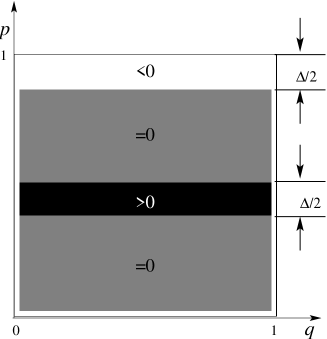
Figure 1: Sechematic representation of the Husimi function $\Gamma(z,z^{*})$ for the noise used in Łoziński et al. (2002). Dissipation takes place where $\Gamma(z,z^{*})\neq 0$.

The operator $A$ defined in Eq. (9) for this model is

$$\Gamma=\frac{1}{N}\left(V^{-N\Delta/2}D_{t}V^{N\Delta/2}-D_{t}\right)$$ (24)

where $V^{N\Delta/2}$ is a translation size $\Delta/2$ in momentum and $D_{t}$ is the projection onto the upper half of the torus. For clarity in FIG. 1, instead of the Weyl representation of $\Gamma$, the corresponding Husimi $\Gamma(z,z^{*})$ is shown. The regions where $\Gamma(z)\neq 0$ are the regions where dissipation takes place.

IV.3 Generalized amplitude damping noises

A large variety of dissipative noise models which are derived from a microscopic Hamiltonian for a system (an oscillator Liu et al. (2004), a rotor Dittrich and Graham (1990), a large spin Haake (1992); Braun et al. (1998), etc) in contact with a bath in thermal equilibrium can be interpreted as generalized amplitude damping models and modeled by the following Kraus superoperator:

$$\text{{{S}}}(\rho)=\sum_{k}A_{k}\rho A_{k}^{\dagger}$$ (25)

where

$$A_{k}=\sum_{n}c_{n}^{k}|n\rangle\langle n+k|$$ (26)

is a combination of the transition operators

$$P_{ij}\stackrel{{\scriptstyle{\rm def}}}{{=}}|i\rangle\langle j|.$$ (27)

Although the basis states $|i\rangle$ and the form of the coefficients $c_{n}^{k}$ depend on each particular problem, a common feature to all these models is that when S acts on the basis of the $P_{ij}$ the skewness $\alpha=(i-j)$ is conserved. With the notation $P_{ij}=P_{i}^{\alpha}$ the evolution of the $P_{l}^{\alpha}$ in each subspace labeled by $\alpha$ is given by

$$\text{{{S}}}P_{i}^{\alpha}=\sum_{l}m_{i,l}^{\alpha}P_{l}^{\alpha}$$ (28)

with $m_{i,l}^{\alpha}=c_{l}^{i-l}c_{l-\alpha}^{i-l*}$.

The preservation of the trace implies that $\sum_{l=0}^{N-1}m_{i,l}^{0}=1$ while the unitality condition corresponds in addition to $\sum_{i=0}^{N-1}m_{i,l}^{0}=1$. It is then clear that in order to analyze the unitality of a noise of this type it is sufficient to study the properties of the $(N\times N)$- matrix $m_{i,l}^{0}$, unitality corresponding to the bistochasticity of this matrix.

It is immediate to see that if the matrix $m_{i,l}^{0}$ is either symmetric, or symmetric with respect to the diagonal $i+j=N-1$ stochasticity implies bistochasticity.

A symmetric matrix corresponds to having a purely diffusive reservoir, i.e., a thermal bath at infinite temperature, exchanging quanta with the system in both directions at equal rate.

In the second case the matrix elements $m_{i,l}^{0}$ only depend on $(i-j)$, implying that in Eq. (26) the coefficients $c_{i}^{k}=c(k)$. Expanding the transition operators in the basis of the translations on the torus $T_{(q,p)}$ (as defined by SchwingerSchwinger (1960)), it is easy to see that the superoperator S is diagonal in this basis

$$\text{{{S}}}\rho=\frac{1}{N^{2}}\sum_{k}c(-k)T_{(k,0)}\rho T^{\dagger}_{(k,0)}$$ (29)

that is, it can be written as an incoherent sum of translations in phase space.

If we compute $\eta$ for this type of models we get:

$$\eta=\sum_{l}(\sum_{i}m_{i,l})^{2}-1.$$ (30)

For the dissipative map studied by Dittrich and Graham in Dittrich and Graham (1990) (adapted to a finite dimensional Hilbert space), this gives in the limit of zero temperature (to second order in $\gamma$)

$$\eta=\gamma^{2}(N-1),$$ (31)

where $\gamma$ is the friction parameter (differential rate of loss of action) of the corresponding classical map (see Eq. (2.4) in Dittrich and Graham (1990)).

V Simple Dissipation Channel

We propose a family of non-unital noise channels to serve as simplified models of dissipative processes like the one described in Sec. IV.3 Let

$$\text{{{D}}}_{\epsilon}(\rho)=(1-\epsilon)\rho+\epsilon\sum_{ij}p_{ij}P_{ij}\rho P_{ij}^{\dagger},$$ (32)

with $P_{ij}$ as in Eq. (27) and $p_{ij}$ real and positive. Equation (32) is in Kraus form and thus $\text{{{D}}}_{\epsilon}$ is CP. The TP condition (6) is

$$\sum_{ij}p^{T}_{ij}P_{ij}^{\dagger}P_{ij} = I$$

$$\sum_{i}P_{ii}\sum_{j}p^{T}_{ij} = I$$ (33)

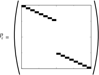
Figure 2: Graphical representation of the structure of the matrix $[p_{ij}]$ with $N=32$ and $\alpha=0.5$. The color scheme is as follows: white means null value and a black square equals one element of value equal to 1.

Figure 3: (Color online) The contracting parameter $\eta$ as a function of $\alpha$ for the dissipation model of Eq. (34) for two different values of $\epsilon$: ($*$) $\epsilon=0.5$, ($\blacktriangle$) $\epsilon=0.75$.

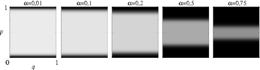
Figure 4: Plot of the Husimi function $\Gamma(z,z^{*})$ for $N=64$ (in gray scale, black is maximum and white minimum) and different values of $\alpha$.Lighter regions indicate local contractive regions.

where $T$ means ‘transpose’.Therefore the matrix of coefficients $p_{ij}$ should be stochastic. If it is doubly stochastic then the noise is unital. This is a model which is diagonal in the $P_{ij}$ representation and decoherence appears as a reduction by a factor $(1-\epsilon)$ of the non-diagonal terms of the density matrix.

We can create dissipative models just by using non-symmetric stochastic matrix of coefficients $p_{ij}$. Consider the family

$$\text{{{D}}}_{\epsilon\alpha}(\rho)=(1-\epsilon)\rho+\epsilon\sum_{i,j=-N/2}^{N/2}P_{[\alpha i]\,i}\rho P_{[\alpha i]\,i}^{\dagger},$$ (34)

with $\alpha\in[0,1)$ and the index $[\alpha i]$ is the integer part of $\alpha i$, as a function of the parameter $\alpha$ and the negative values are taken mod$(N)$. In FIG. 2 there is an illustration of the structure of the matrix $[p_{ij}]$ of Eq. (32) for the case $\alpha=0.5,N=32$.

For all values of $\alpha$, the first term attenuates uniformly the off-diagonal elements of the density matrix, introducing decoherence. The second term which acts on the probabilities (diagonal elements) takes the system to lower states. The permitted transitions of the diagonal elements are determined by the parameter $\alpha$ but its dependence on the parameter $\epsilon$, which accounts for the coupling strength of the system to the environment, becomes important when the contraction is considered.

If $P{ij}$ are transitions in the computational basis of a state of say $k=\log_{2}N$ qubits, then the noise can be interpreted as follows. With probability $(1-\epsilon)$ it leaves the initial state untouched while with probability $\epsilon$ it induces errors in the form of transitions which depend on the parameter $\alpha$. For $\alpha=1$ the superoperator is unital and corresponds to a phase damping channel for $k=\log_{2}N$ qubits . If $\alpha<1$ this very simple model captures some important features of the amplitude damping noises (an example of which is described in Sec. IV.3). On the other hand, if we take $P_{ij}$ to be transitions in momentum and since the invariant state (for all $\alpha\neq 0$) is $\rho^{*}=P_{00}=|p=0\rangle\langle p=0|$ then the noise has the effect of a friction. As is shown later, in phase space representation the parameter $\alpha$ is related to the region over which dissipation acts.

The simple form of Eq. (34) allows to compute the contraction parameter easily as

$$\eta = N{\rm Tr}\left[(\text{{{D}}}_{\epsilon\alpha}(I/N)-I/N)^{2}\right]$$ (35)

$$= \frac{\epsilon^{2}}{N}{\rm Tr}\left[I-2\sum_{i}P_{[\alpha i],[\alpha i]}+\sum_{ij}P_{[\alpha i],[\alpha i]}P_{[\alpha j],[\alpha j]}\right]$$

$$= \frac{\epsilon^{2}}{N}{\rm Tr}\left[\sum_{ij}|\langle\alpha j|\alpha i\rangle|^{2}-N\right]$$

where $\sum_{i}P_{[\alpha i],[\alpha i]}=N$ and for simplicity we drop the $[\ ]$ symbol inside the kets and bras. Now $\langle\alpha j|\alpha i\rangle=0,1$ so the square can be dropped and in order to calculate the sum we approximate by continuous variables as

$$\sum_{ij}\langle\alpha j|\alpha i\rangle \sim \iint\delta(\alpha(x_{i}-x_{j}))\simeq{1\over\alpha}\iint\delta(x_{i}-x_{j})$$ (36)

$$\sim {1\over\alpha}\sum_{ij}\delta_{ij}=\frac{N}{\alpha}.$$

Therefore we get

$$\eta=\epsilon^{2}\left(\frac{1-\alpha}{\alpha}\right).$$ (37)

In figure FIG. 3we plot $\eta(\alpha,\epsilon)$ for two different values of $\epsilon$. We see that the computed points fit exactly the analytic expression. Moreover the saturation value,

$$\eta(\alpha=1/N,\epsilon)=\epsilon^{2}(N-1).$$ (38)

for small $\alpha$ can be understood as follows. Since the dimension of Hilbert space is $N$ then the integer part $[\alpha\,i]$ ($i=0,\ldots N-1$) for any value of $\alpha<1/N$ is zero. We notice that the dependence on the coupling parameter $\epsilon$ is the same as the one given in Eq. (31) for the dissipative map of Dittrich and Graham (1990), if one identifies it with the friction parameter $\gamma$. In addition, it can be easily seen by taking the mean values of $p$ and $q$ that this operation implies the following dissipative map in the classical limit

$$\begin{array}[]{rcl}\bar{q}^{\prime}&=&\bar{q}\\ \bar{p}^{\prime}&=&(1-\epsilon)\bar{p}\end{array}$$ (39)

where the bar indicates mean values.

For this model the operator $\Gamma$ defined in Eq. (9) is

$$\Gamma=\epsilon\sum_{i=-N/2}^{N/2}\left(P_{[\alpha i][\alpha i]}-P_{ii}\right).$$ (40)

So the region of dissipation (determined by a negative value of $A$) has area equal to $1-\alpha$, and occupies the central region of the unit square. In figure FIG. 4 the Husimi function of the operator $\Gamma$ is represented taking different values of $\alpha$ (and $\epsilon=0.5$). The light region represents the area where contraction takes place and corresponds to a negative value of $\Gamma$. For $\alpha\sim 0$ the contraction is uniform over (almost) all phase space, except over the state $|0\rangle$ of momentum.

VI Composition with a Unitary Process

Following recent worksBianucci et al. (2002); García-Mata et al. (2003); García-Mata and Saraceno (2004); Nonnenmacher (2003); Łoziński et al. (2002); Braun (1999, 2001) we study the effect of the dissipative noise channel described in Sec. V when composed with a unitary map. As an example we take the quantum version of the standard map on the torus. We suppose that to a good approximation the whole noisy propagation takes place in two steps

$$\text{{{S}}}(\rho)=\text{{{D}}}_{\epsilon\alpha}(\text{{{U}}}(\rho))$$ (41)

where $\text{{{U}}}(\rho)=U\rho U^{\dagger}$ is the unitary step. The two-step scheme can can be used, in the master equation if the Hamiltonian part commutes, to some desired order in $\hbar$ with the non-Hamiltonian part. In the quantum operation formalism these scheme is suitable in the case for example where unitary evolution takes place in so short times that the noise is negligible (e.g. the micro-maser, a billiard where the interaction with the walls is very short and the evolution inside is dissipative).

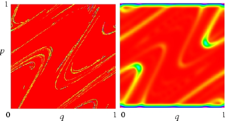
Figure 5: (Color online) Left: histogram representation of the attractor for the classical standard map (Eq. (42) with $k=0.065,\delta=0.6$) with dissipation. Right: Husimi representation for invariant state for the quantum standard map with the dissipative noise described in Sec. V ($\alpha\sim 0,\epsilon=0.4$

The unitary map chosen is the quantum version of the standard map on the torus

$$q^{\prime} = q+p^{\prime}$$ (42)

$$p^{\prime} = \delta p-2\pi k\sin(2\pi q)$$ (43)

where the factor $\delta<1$ on the momentum acts as friction.

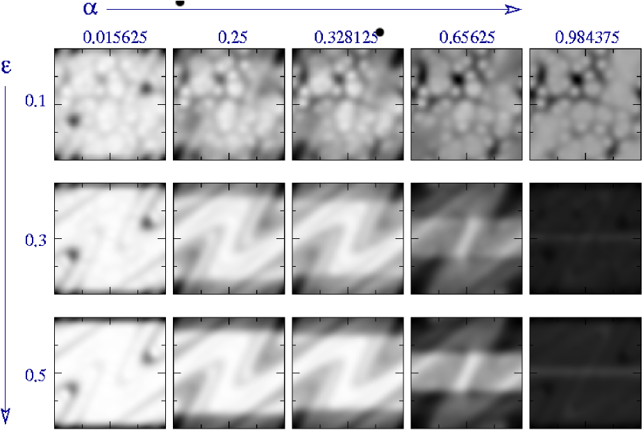
Figure 6: Husimi representation (same color scheme as FIG. 4) of the invariant state for the standard map with dissipation for different values of $\alpha$ and $\epsilon$ and $N=64$. The difference between $\alpha\approx 0$ (dissipation) and $\alpha\approx 1$ (diffusion) can be observed. (Axes and units are the same as in FIGS. 4 and FIG. 5.)

In FIG. 5 the classical and quantum invariant states are plotted. The classical attractor on the left is represented as density in phase space. On the right is the Husimi distribution of the invariant state for the quantum version of the map followed by the noise of Eq. (34) for $\alpha\sim 1/N$ ($N=64$). Since the dissipation terms in Eqs. (39) and (42) are the same when $\delta=(1-\epsilon)$, as expected the quantum invariant state exhibits the structure of the classical attractor.

The shadow on the lower and upper edge of the torus can be explained from the definition of $\Gamma$, Eq. (40), for this noise (corresponding to the rightmost image in FIG. 4). The same argument can be used to explain FIG. 6. As $\alpha$ grows the region of dissipation becomes smaller as well as the contracting parameter $\eta$. The noise becomes increasingly similar to a unital operation, at least on the upper and lower bands of width $\alpha/2$. So over the black shaded regions of FIG. 6 the noise acts like a generalized phase damping channel Aolita et al. (2004), where the preferred basis are the momentum projectors $P_{ii}$ with $i=\{0,\ldots,\alpha N/2\}\cup\{(1-\alpha/2)N-1,\cdots,N-1\}$, while on the lighter region, a dissipation of the type of Eq. (39) acts and the attractor is uncovered.

VII Conclusions

The fundamental difference between unital and non-unital processes was explored. In analogy to the classical limit of the master equation, which relates the commutator of the Lindblad operators to the vector drift in its Fokker-Planck limit, we defined a parameter that measures non-unitality and characterizes dissipative quantum operations. As an example we proposed a noise channel that displays in a simple way the essential features of decoherent and dissipative processes.

The non-unitality of the superoperator is related to a traceless Hermitian operator whose phase space distribution gives a local image of the dissipation process. This operator is independent on the Kraus representation and can give a useful insight into the dissipative properties of the superoperator when a phase space description or a semiclassical limit is not available, like for general noise channels in quantum information.