Atomic density of a harmonically trapped ideal gas near Bose-Einstein transition temperature

Abstract

We have studied the atomic density of a cloud confined in an isotropic harmonic trap at the vicinity of the Bose-Einstein transition temperature. We show that, for a non-interacting gas and near this temperature, the ground-state density has the same order of magnitude as the excited states density at the centre of the trap. This holds in a range of temperatures where the ground-state population is negligible compared to the total atom number. We compare the exact calculations, available in a harmonic trap, to semi-classical approximations. We show that these latter should include the ground-state contribution to be accurate.

The phenomenon of Bose-Einstein condensation (BEC) is a phase transition. Below the critical temperature $T_{c}$, the ground-state population, which is the order parameter, becomes macroscopic. This phenomenon, that happens strictly speaking only at the thermodynamic limit, is usually illustrated in textbooks with a homogeneous gas. Experimentally, the Bose-Einstein condensation of dilute gases has been observed since 1995 with atoms confined in a harmonic trap Varenna . These stimulating experimental data have quickly pointed out that two effects had to be taken into account: the interatomic interactions and the finite number of atoms stringari-revue . Several papers, as the present one, have studied harmonically trapped ideal gases containing a finite number of atoms. Two quantities have been investigated in detail: the atom number grossmann ; ketterle ; stringari ; darnval ; giorgini ; pathria and the specific heat inc ; darnval ; pathria . For a finite but large (typically $10^{6}$) number of atoms, the properties of the atomic cloud change abruptly at a characteristic temperature we will name the transition temperature $T^{*}$. This temperature is shifted compared to $T_{c}$, but by a small amount, typically of few percent for atom numbers around $10^{6}$. There is also a characteristic temperature for the specific heat; it is different from the previous one but still close to $T_{c}$ inc ; pathria .

Surprisingly, less attention has been paid on the atomic density of an ideal gas krauth96 . In a homogeneous gas it is obviously equivalent to the atom number but this is no more the case in a spatially varying potential. It becomes the good parameter of the theory, in particular to perform local density approximations. This quantity is then particularly important for the study of the shift of the critical temperature by the interatomic interactions, both within the mean-field approximation stringari and beyond this approximation arnold2 . We will show, in the case of an isotropic harmonic trapping and for a finite atom number, that the ground-state density at the centre of the trap increases much more sharply than its population as the temperature decreases. This leads to the fact that near the Bose-Einstein transition temperature the density is already dominated by the ground-state contribution. This holds whatever the atom number is, and is a remanence of the infinite compressibility of an ideal gas at the thermodynamic limit compressibilite . Usual semi-classical approximations do not take into account the ground-state contribution and then fail in the vicinity of the Bose-Einstein transition temperature. This is not a finite size effect in the sense that it is not related to the discretization of the excited states energy levels. We will compare the exact results with semi-classical approximations. The addition of the ground-state contribution on the latter ones improves their accuracy. We will finally show that the influence of the ground-state is smaller if the measured quantity is the density integrated over at least one dimension. It is still large for typical experimental parameters.

We will perform our calculations in the grand canonical ensemble (GCE). Then, the Bose-Einstein distribution gives the population $N_{i}$ of a given energy level $\epsilon_{i}$: $N_{i}=(e^{\beta(\epsilon_{i}-\mu)}-1)^{-1}$ with $\sum\limits_{i=0}^{\infty}N_{i}=N$. Here $\beta=1/k_{B}T$ with $k_{B}$ the Boltzmann’s constant, $\mu$ the chemical potential and $N$ the total atom number. The equivalence between GCE and the canonical or microcanonical ensemble, these latter being probably more appropriate descriptions, is generally not guaranteed, especially for systems that are not at the thermodynamic limit. For instance, it is well known that the GCE predicts unphysical large fluctuations of the condensate population at low temperature landau . However, the authors of Ref. krauth96 ; Politzer96 ; Olshanii97 have shown that the occupation numbers $N_{i}$ in GCE are very close to the ones in the canonical ensemble. The difference is more pronounced for small atom number and anisotropic clouds. As a result and because GCE enables to give analytic expressions on contrary to the other ensembles, we will use GCE in the following.

For a fixed atom number, the chemical potential increases as the temperature decreases. As $\mu$ has to be smaller than $\epsilon_{0}$, the ground-state energy, the excited states population will saturate when $\mu$ approaches $\epsilon_{0}$ whereas $N_{0}$ is still increasing: $N-N_{0}=\sum\limits_{i=1}^{\infty}N_{i}(\mu,T)\leq\sum\limits_{i=1}^{\infty}N_{i}(\epsilon_{0},T)$. As in Ref. stringari-revue ; castin , we will define the transition temperature $T^{*}$ as the temperature for which the excited states saturated population is equal to the total atom number:

$$\sum\limits_{i=1}^{\infty}N_{i}(\epsilon_{0},T^{*})=N$$ (1)

As pointed out in the introduction, there is not a unique definition of the transition temperature for a finite atom number. Other definitions use, for instance, a change in the slope for the condensate fraction in function of temperature (more explicitly $\frac{d^{3}(N_{0}/N)}{dT^{3}}=0$) Bergeman , a change in the power dependence on the condensate fraction in function of the atom number pathria , which are also pertinent. We have checked that these various definitions affect marginally the value of $T^{*}$ and do not modify our conclusions resTc . In the following we will then use Eq.(1) to define $T^{*}$. Note that the chemical potential $\mu^{*}$ at the transition temperature is close but not equal to the ground-state energy; it is determined by the constraint

$$\sum\limits_{i=0}^{\infty}N_{i}(\mu^{*},T^{*})=N$$ (2)

There are only a few examples of trapping potentials where the eigen-energies and the eigen-functions are known exactly. Semi-classical approximations give usually accurate enough results and are suited to include interatomic interactions, at least perturbatively. We will derive various type of semi-classical approximations in the following and test their accuracy because the harmonic potential is an exactly solvable potential.

We will first examine the situation where $\hbar\omega\ll k_{B}T$ with $\omega$ the oscillation frequency of the isotropic harmonic trap. This corresponds to the large atom number limit and semi-classical approximations should work. Replacing the discrete energy spectrum by a continuous one and neglecting the ground-state energy $\epsilon_{0}$, the density is $\rho(r)={1\over\lambda^{3}}g_{3\over 2}[z\exp(-{\tau\over 2}(r/\sigma)^{2}]$ with $z=e^{\beta\mu}$ the fugacity, $\tau={\hbar\omega\over k_{B}T}$ and $g_{3\over 2}()$ a Bose function bose . With the above notation, the thermal de Broglie wavelength is $\lambda=\sigma\sqrt{2\pi\tau}$ and the size of the cloud is $\sqrt{{k_{B}T\over m\omega^{2}}}=\sigma/\sqrt{\tau}$. Similarly, the atom number is $N=g_{3}(z)/\tau^{3}$. Equation (1) leads then to $N=\zeta(3)/{\tau^{*}}^{3}$, with $\tau^{*}$ the value of $\tau$ at $T=T^{*}$. The above expressions for the density and atom number are in fact approximations for the excited states and do not contain the ground-state contribution. Then $\mu^{*}$ defined by Eq.(2) is equal to 0 and $z^{*}=1$. The transition temperature defined here corresponds to the critical temperature $T_{c}$. The peak density at the transition temperature is then given by $\rho(0)\lambda^{3}=g_{3\over 2}(z^{*})=\zeta(3/2)\approx 2.612$. For temperatures below $T_{c}$, the excited states population is given by $\zeta(3)/\tau^{3}$. Then, the ground-state population fraction is $N_{0}/N=0$ for $T>T_{c}$ and $N_{0}/N=1-(T/T_{c})^{3}$ for $T<T_{c}$. This fraction will be plotted in fig.1, labelled with $sc_{\infty}$.

These approximations are too crude and give inaccurate results for the atomic density, however. The reason is that the ground-state contribution cannot be neglected. A better expression is $\rho(r)={1\over\lambda^{3}}g_{3\over 2}[ze^{-{\tau\over 2}(r/\sigma)^{2}}]+\rho_{0}(r)$ and similarly $N={1\over\tau^{3}}g_{3}(z)+N_{0}$ with $\rho_{0}(r)={N_{0}\over(\sqrt{\pi}\sigma)^{3}}e^{-(r/\sigma)^{2}}$ and $N_{0}={z\over 1-z}$. The value of $T^{*}$ is unchanged as it is defined by the excited states saturation, but $z^{*}$ is now different from 1. Using $g_{3}(z^{*})\approx\zeta(3)-\zeta(2)x^{*}$ with $z^{*}=e^{-x^{*}}$ ($x=\beta(\epsilon_{0}-\mu)>0$), one finds using Eq.(2) that $x^{*}\approx{\tau^{*}}^{3/2}/\sqrt{\zeta(2)}$ pathria . The ground-state population is $\sim 1/x^{*}$ and, as expected, is vanishingly small as $\tau^{*}\rightarrow 0$ compared to the excited-state population $\zeta(3)/{\tau^{*}}^{3}$. The ground-state peak density is $\sim{1\over(\sqrt{\pi}\sigma)^{3}x^{*}}$ whereas the excited state peak density is $\zeta(3/2)/{\lambda^{*}}^{3}$. As $\lambda^{*}=\sigma\sqrt{2\pi\tau^{*}}$, the two quantities have the same order of magnitude! The above high-N analysis predicts then that the degeneracy parameter at the transition temperature is $\rho(0)\lambda^{3}=\zeta(3/2)+2\sqrt{2\zeta(2)}\approx 6.24$ and not 2.612. The ground-state population is extremely small but the size of its wave-function is also extremely small compared to the atomic cloud size. For a harmonic trap both depend on the same small parameter, raised to the same power. So, even for very large atom number, the traditional criterion for BEC should be modified. This effect is linked to the pathological behaviour of the ground-state density at the thermodynamic limit, i.e. the infinite compressibility of an ideal gas compressibilite . This limit means $N\rightarrow\infty$ with $N\omega^{3}\rightarrow$ constant. The ground-state size being $\sigma=\sqrt{\hbar/m\omega}$, the density of that state behaves as $\sqrt{N}$ below threshold and is then infinite at the thermodynamic limit whereas the density above $T_{c}$ is finite.

We will now address the case of atom numbers in the accessible experimental range, $10^{3}-10^{6}$. It is well known that the transition temperature will be shifted compared to $T_{c}$ grossmann ; ketterle ; darnval . A better approximation, which takes into account the ground-state energy to first order, is $\rho(r)={1\over\lambda^{3}}\{g_{3\over 2}[\tilde{z}(r)]+{3\tau\over 2}g_{1\over 2}[\tilde{z}(r)]\}$ where $\tilde{z}(r)=ze^{-{\tau\over 2}(r/\sigma)^{2}}$. Then $N={1\over\tau^{3}}[g_{3}(z)+{3\tau\over 2}g_{2}(z)]$. The corresponding transition temperature is $T^{*}_{sc}$ such that $N={1\over\tau^{*3}_{sc}}[\zeta(3)+{3\over 2}\zeta(2)\tau^{*}_{sc}]$. This is the usual semi-classical approximation found in the literature. The ground-state population fraction is then $N_{0}/N=0$ for $T>T^{*}_{sc}$ and $N_{0}/N=1-({T\over T^{*}_{sc}})^{3}\frac{\zeta(3)+{3\tau\over 2}\zeta(2)}{\zeta(3)+{3\tau^{*}_{sc}\over 2}\zeta(2)}$ for $T<T^{*}_{sc}$. This fraction, also plotted in fig.1, will be labelled with $sc_{0}$. Note that $g_{1\over 2}(z)$ diverges at $z=1$ Yukalov05 , meaning that this approximation is intrinsically inaccurate near the centre of the trap and near the transition temperature. This divergence is however weak, and any spatial integration would give a finite result. We can still cure this pathology by adding, as before, the ground-state contribution. We obtain then

$$\left\{\!\!\!\begin{tabular}[]{l}$\rho_{sc}(r)={1\over\lambda^{3}}\{g_{3\over 2}[\tilde{z}(r)]+{3\tau\over 2}g_{1\over 2}[\tilde{z}(r)]\}+{z\over 1-z}{e^{-({r\over\sigma})^{2}}\over(\sqrt{\pi}\sigma)^{3}}$\\ $N={1\over\tau^{3}}[g_{3}(z)+{3\over 2}\tau g_{2}(z)]+{z\over 1-z}$\\ $T^{*}_{sc}$ such that $N={1\over\tau^{*3}_{sc}}[\zeta(3)+{3\over 2}\zeta(2)\tau^{*}_{sc}]$\end{tabular}\right.$$ (3)

This semi-classical approximation will be labelled with $sc$ in the following. The comparison of $T^{*}_{sc}$ with the value given by the exact model (see below) can be used to check the finite size correction. Even so, this comparison is useless to check the contribution coming from the ground state since it does not depend on it (same transition temperature as $sc_{0}$).

We can now test these semi-classical approximations for a harmonically trapped gas. As we referred before, for this case, the eigen-energies and the eigen-functions are known exactly. The corresponding expressions of the atomic density and atom number landau , labelled with $ex$ in the following, are :

$\left\{\begin{tabular}[]{l}$\rho_{ex}(r)={1\over(\sqrt{\pi}\sigma)^{3}}\sum\limits_{l=1}^{\infty}{z^{l}\over(1-e^{-2\tau l})^{3/2}}\;e^{-\tanh({\tau l\over 2})({r\over\sigma})^{2}}$\\ $N=\sum\limits_{l=1}^{\infty}{z^{l}\over(1-e^{-\tau l})^{3}}$\\ $T^{*}_{ex}$ such that $N=\sum\limits\limits_{l=1}^{\infty}({1\over(1-e^{-\tau^{*}_{ex}l})^{3}}-1)$\end{tabular}\right.$
where, here $z=e^{\beta(\mu-\epsilon_{0})}$. The semi-classical model corresponds to a Taylor expansion in $\tau$ of these last expressions.

In fig.1 we plot the ground-state population fraction in function of the temperature for the various models described above. When the number of atoms is only $10^{3}$, finite size effects are large. The prediction of model $sc_{\infty}$ is clearly wrong compared to the exact model prediction. On contrary models $sc_{0}$ and $sc$ give a result close to the one of $ex$ calcul . Figure 2 shows the relative deviations of $T_{c}$ and $T^{*}_{sc}$ from $T^{*}_{ex}$ in function of the atom number. As expected the different values are similar but, as above, the model $sc$ give a closer result to $ex$ than $sc_{\infty}$. The value $T^{*}_{sc}$ deviates less than $1\%$ for $N>400$ and the relative shift is $\sim 10^{-4}$ for typical experimental atom numbers. This is well below actual experimental uncertainties. The thermodynamic value $T_{c}$ deviates more, typically 1 % but is still close to $T_{ex}^{*}$ grossmann ; ketterle ; darnval ; pathria . The discrepancy with $T_{c}$ would have been more pronounced for an anisotropic trap (see below).

This two figures illustrate what is called finite size effects, the fact that the energy level spacing is not negligible compared to the temperature. What we are interested in is the role of the ground-state. For this, the transition temperature and the condensate population fraction are not the best observables. It is nevertheless already clear from fig.1 that $sc$ is a significant improved model to describe semi-classically a cloud near degeneracy compared to $sc_{0}$. The high-N model predicts that the ground-state influence should be much more pronounced on the peak density. We will now focus our attention on that observable, only in the more pertinent comparison between the models $sc$ and $ex$.

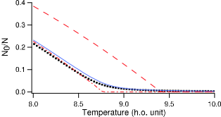
Figure 1: Ground-state population fraction in function of the temperature in $\hbar\omega/k_{B}$ unit for a cloud of $10^{3}$ atoms. The dotted curve corresponds to the exact result given by model $ex$. The solid, dot-dashed and dashed lines correspond respectively to the semi-classical models $sc$, $sc_{0}$ and $sc_{\infty}$. The last two neglect the ground-state contribution above their corresponding transition temperature and the first two take into account finite size effects. The model $sc$ is the closest to $ex$ near Bose-Einstein transition.

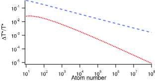
Figure 2: Relative shift of the semi-classical transition temperatures $T_{c}$ (dashed line) and $T_{sc}^{*}$ (dotted line) to $T_{ex}^{*}$ (see text) in function of the atom number. Both temperatures converge for high atom numbers. The critical temperature at thermodynamic limit, $T_{c}$, deviates by less than $1\%$ for $N>5\,10^{5}$. The semi-classical transition temperature defined for a finite atom number, $T_{sc}^{*}$, is much more accurate and deviates by less than $1\%$ for $N>400$.

This is first illustrated on fig. 3 where the degeneracy parameter $\rho(0)\lambda^{3}$ is plotted in function of the atom number for clouds at $T=T^{*}$. We plot this number for the semi-classical approximation $sc$ and for the exact model, $ex$. The two curves are higher than $2.612$. This highlights the inaccuracy of the standard semi-classical models ($sc_{0}$ or $sc_{\infty}$) that do not take into account the ground-state contribution. It confirms also the calculation developed above. The degeneracy parameter is astonishingly constant till $10^{3}$ atoms and does not differ much even for smaller atom numbers. Models $sc$ and $ex$, which have almost the same transition temperature, have the same asymptotic value of the degeneracy parameter. This value, $6.24$, is the one predicted by our high-N analysis. The model $sc$ is significantly higher than this value for experimentally accessible atom numbers. This is because our first analysis does not take into account the ${3\over 2}\tau$ term of model $sc$. To first order bose , $x^{*}_{sc}\approx{(\tau_{sc}^{*})^{3\over 2}\over\sqrt{\zeta(2)}}(1+{9\over 8\zeta(2)}\tau^{*}_{sc}\ln\tau^{*}_{sc})$ and is then slightly smaller than $(\tau_{sc}^{*})^{3\over 2}\over\sqrt{\zeta(2)}$. Consequently the ground-state peak density is bigger at $T^{*}_{sc}$ using model $sc$ than at $T_{c}$ using the high-N model. The excited states peak density is also higher in model $sc$ because of this ${3\over 2}\tau g_{1\over 2}$ term.

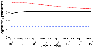
Figure 3: Degeneracy parameter $\rho(0)\lambda^{3}$ in function of the atom number $N$ for clouds at the transition temperature. The dotted line corresponds to the semi-classical model $sc$ at $T=T_{sc}^{*}$ and the solid line to model $ex$ at $T=T_{ex}^{*}$. Even if the degeneracy parameters are somewhat different, they both differ significantly to the usual value of 2.612 (dashed horizontal line). This deviation is due to an under-estimation of the ground-state density. The actual values are close to our high-N prediction of 6.24 (see text).

The next three figures deal with the cloud properties around the Bose-Einstein threshold. Figure 4 and fig.5 show the evolution of the condensate fraction $N_{0}/N$ and the condensate peak density fraction in function of $T$ for two different atom numbers, $10^{6}$ and $10^{3}$. Figure 6 shows the density profile of clouds near degeneracy. What prevails in fig.4 is the sharp increase of the condensate peak density compared to the condensate population. Moreover the models $sc$ and $ex$ give very close results validating our analysis on the ground-state contribution near degeneracy. This means that the peak density is a much better marker of the Bose-Einstein threshold than the atom number. This feature is in fact used experimentally: the appearance of a small peak over a broad distribution is the usual criterion to distinguish clouds above or below the transition temperature. This sharpness also explains why the value of the peak density is very sensitive to the value of the temperature (cf. fig.3). Figure 4 shows also that, above threshold, the ground-state peak density fraction decays slowly. This is even more pronounced in fig.5 where $N=10^{3}$ instead of $10^{6}$. It comes from the fact that the number of populated states is not macroscopic anymore ($k_{B}T<10\hbar\omega$) and then the transition is smoother for smaller atom number. Once again, the density is a better marker of degeneracy than the atom number. This figure shows also that the ${3\over 2}\tau$ term and the ground-state contribution make the model $sc$ still very close to model $ex$, respecting the density and population fractions, even for $10^{3}$ atoms.

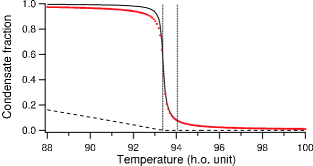
Figure 4: Condensate atom number fraction $N_{0}/N$ (dashed line) and peak density fraction $\rho_{0}(0)/\rho(0)$ (solid line) in function of the temperature in harmonic oscillator unit $\hbar\omega/k_{B}$, using model $ex$. The cloud contains $10^{6}$ atoms. The transition temperature is $T_{ex}^{*}=93.37\hbar\omega/k_{B}$ and the asymptotic thermodynamic temperature is $T_{c}=94.05\hbar\omega/k_{B}$. The positions of these temperatures are shown as vertical lines in the figure. The ground-state peak density increases much more sharply than the ground-state population around the transition temperature. The former has also a significant value above $T^{*}_{ex}$. The model $sc$ is indistinguishable for $N_{0}/N$, but is slightly different for $\rho_{0}(0)/\rho(0)$ (dotted line).

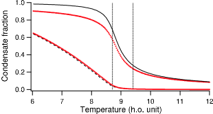
Figure 5: Same as in Fig.4 but with $10^{3}$ atoms. The transition temperature is $T_{ex}^{*}=8.71\hbar\omega/k_{B}$ and the asymptotic thermodynamic temperature is $T_{c}=9.41\hbar\omega/k_{B}$. Since the number of populated states is considerably reduced compared to fig.4, the discrepancy between $sc$ (dotted lines) and $ex$ is more pronounced. This also explains why the increase of the condensate peak density is slower.

The above analysis is focused on the peak density i. e. at the centre of the cloud. Figure 6 shows the total density profile of clouds, all at the same temperature, but containing different numbers of atoms around $N^{*}_{ex}$, the number of atoms for which $T=T^{*}_{ex}$ ($N=N^{*}_{ex}$ corresponds to the dotted line). This figure simulates somehow an experimental observation of BEC threshold. Only the central part is sensitive to the atom number; this corresponds to the condensate growing as the number of atoms is increased and to the fact that the excited states are already saturated for these atom numbers. Moreover, by looking at the graph, one would rather think that the Bose-Einstein transition occurs for a smaller atom number. This points out that the definition on the transition temperature based on an atom number criterion does not fully correspond to the one based on the atomic density which would be more connected to experiments. The inset shows the excited states and ground state density profiles at threshold. The excited states density exhibits a dip in the centre of the cloud, obviously not present in semi-classical models (monotonic functions). We check that the height of the dip is proportional to $1/\tau$ and can almost be totally attributed to the first excited state population. The aim of this paper is to show the importance of the ground-state in the study of non-interacting clouds close to threshold. The inset reveals that the first excited state density is also largely under-estimated; it represents $\sim 10~{}\%$ of the peak density whereas it contributes only to $\sim 0.1~{}\%$ of the population.

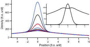
Figure 6: Atomic density $\rho_{ex}$ in function of $r/\sigma$ where $\sigma$ is the size of the harmonic oscillator ground-state. The temperature is $T=93.37\hbar\omega/k_{B}$ and the atom number $N$ spans from $0.990\;10^{6}$ to $1.004\;10^{6}$ by step of $2000$ atoms. The curve at threshold is in dotted line and corresponds to $10^{6}$ atoms. The inset shows the excited states and ground state density profile at threshold. The dip around $r=0$ is mainly due to the first excited state population.

We have shown results on the atomic density at the vicinity of the transition temperature. Detection techniques consist rather on 1D-integrated density, corresponding to 2D absorption images, or 2D-integrated density BecHe . One can show that, at threshold, the 1D and 2D-integrated peak density of the ground-state are vanishingly small for large atom numbers on contrary to the non-integrated case. The peak 1D-integrated density fraction behaves at threshold as $\sqrt{\tau}$ and the 2D-integrated peak density as $\tau$. For typical atom number this is nevertheless not negligible. This is illustrated in Fig.7 where is plotted the condensate peak density fraction for 3D, 2D and 1D images of clouds at threshold. The calculations use the model $ex$. At the transition temperature $T^{*}_{ex}$, the ground-state contributes to more than $10\%$ for $N<2500$ atoms in 1D images and for $N<8\;10^{6}$ atoms for 2D images. It means that, even with the conventional technique of absorption images, the effect should be experimentally observable if interactions could be switched off using, for instance, the magnetic tunability of the scattering length close to a Feshbach resonance feshbach .

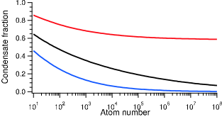
Figure 7: Contribution of the ground-state on the peak density for, from bottom to top, 1D, 2D and 3D images in function of the number of trapped atoms. The clouds are at the transition temperature $T^{*}_{ex}$ and the calculations use model $ex$. A 3D image would give the density in all three dimensions of space nous whereas a 2D (resp. 1D) image corresponds to the density integrated over one (resp. 2) dimension. For $N=10^{4}$ atoms the ground-state contributes to $\sim 26\%$ in 2D images and $\sim 6\%$ in 1D images. In contrast to 3D image, the ground-state contribution is very small for large atom number; it is not for typical atom numbers accessible in experiments.

Apart from the atomic density, two- and three-body inelastic loss rates will also be affected and could be 20 to 30 % higher than predicted by model $sc_{0}$ around the transition temperature for typical atom numbers. Finally, in most experimental set-ups, the trapping potential is anisotropic and finite size effects are then stronger. Indeed the term ${3\over 2}\tau$ in Eq.(3) should be replaced by ${3\over 2}\frac{\tilde{\omega}}{\bar{\omega}}\tau$, with $\bar{\omega}=(\prod\limits_{i}\omega_{i})^{1/3}$ the geometric mean and $\tilde{\omega}={1\over 3}\sum\limits_{i}\omega_{i}$ the arithmetic mean grossmann . Whatever the anisotropy is, $\tilde{\omega}$ is always larger than $\omega$, making the finite size contribution stronger. To first order and if $k_{B}T^{*}_{ex}\gg\hbar\omega_{i}$ for $i=x,y$ and $z$, the ground-state contribution should be the same since our high-N analysis does not depend on any anisotropy.

In conclusion, we have shown that the density of an ideal atomic gas is dominated by the ground-state contribution near the transition temperature. The inter-atomic interactions have been neglected in our analysis and will modify our conclusions. With repulsive interactions, the clouds tends to decrease its density at the centre of the cloud whereas it tends to increase it with attractive interactions. Previous calculations have treated separately finite size and interactions effects, both corrections being finally added stringari . Since the ground-state has a non-perturbative effect on the density, our analysis tends to prove that both effects have to be investigated together. The approach of Ref.krauth96 could in this respect provide helpful informations. Feshbach resonances, which enable to tune the interactions strength, constitute a powerful tool to check the accuracy of the different theoretical models. Moreover, a full three-dimensional density measurement would also be valuable; this type of measurement is at the edge to be available in our experiment on metastable helium in Orsay nous .

- (1) Proceedings of the International School of Physics ”Enrico Fermi”, Course CXL, edited by M. Inguscio, S. Stringari, C. E. Wieman, IOS Press, Amsterdam (1999).
- (2) F. Dalfovo, S. Giorgini, L. P. Pitaeskii, S. Stringari, Rev. Mod. Phys 71, 463 (1999).
- (3) S. Grossmann and M. Holthaus, Z. Naturforsch. Teil A 50, 921 (1995).
- (4) W. Ketterle and N. J. van Druten, Phys. Rev. A 54, 656 (1996).
- (5) K. Kirsten and D. J. Toms, Phys. Rev. A 54, 4188 (1996).
- (6) S. Giorgini, L. P. Pitaevskii and S. Stringari, Phys. Rev. A 54, R4633 (1996).
- (7) H. Haugerud, T. Haugest and F. Ravndal, Phys. Lett. A 225, 18 (1997).
- (8) S. Giorgini, L. P. Pitaevskii and S. Stringari, J. Low Temp. Phys. 109, 309 (1997).
- (9) R. K. Pathria, Phys. Rev. A 58, 1490 (1998).
- (10) W. Krauth, Phys. Rev. Lett. 77, 3695 (1996).
- (11) P. Arnold and B. Tomàs̆ik, Phys. Rev. A 64, 053609 (2001).
- (12) K. Huang, Statistical Mechanics, Wiley ((1987).
- (13) L. D. Landau and E. M. Liftshiz, Statistical Physics, Butterworths (1996).
- (14) H. D. Politzer, Phys. Rev. A 54, 5048 (1996).
- (15) C. Herzog and M. Olshanii, Phys. Rev. A 55, 3254 (1997).
- (16) Y. Castin, lecture note in ”Coherent atomic matter waves”, Les Houches Session LXXII, eds. R. Kaiser, C. I. Westbrook and F. David, Springer (2001).
- (17) T. Bergeman, D. L. Feder, N. L. Balazs, B. I. Schneider, Phys. Rev. A 61, 063605 (2000).
- (18) In Ref.pathria , the transition temperature was indeed (see later in the text). The transition temperature defined by the maximum of the second derivative of the condensate fraction has been calculated for atom number in the range ; the relative deviation is below on the transition temperature and on the condensate peak density fraction.
- (19) We use the usual definition of Bose functions . We remind that with the Riemann Zeta function. Note that and .
- (20) After submission of this article, we have been aware of a different type of semi-classical approximations which does not give rise to divergences. See V. I. Yukalov, Phys. Rev. A 72, 033608 (2205).
- (21) We use the result of Ref. robinson for the calculation of the Bose functions near the transition temperature. For the series in model , the convergence is very slow but can easily be accelerated. For instance, it is much better to write because the second term converges for large because of the part and because of the part.
- (22) J. E. Robinson, Phys. Rev. 83, 678 (1951).
- (23) A. Robert, O. Sirjean, A. Browaeys, J. Poupard, S. Nowak, D. Boiron, C. I. Westbrook, and A. Aspect, Science 292, 461 (2001); published online 22 march 2001 (10.1126/science.1060622).
- (24) V. Vuletic, A. J. Kerman, C. Chin, S. Chu, Phys. Rev. Lett. 82, 1406 (1999).
- (25) M. Schellekens, R. Hoppeler, A. Perrin, J. Viana Gomes, D. Boiron, A. Aspect, and C. I. Westbrook, Science 310, 648 (2005); published online 15 september 2005 (10.1126/science.1118024).