Field-free two-direction alignment alternation of linear molecules by elliptic laser pulses

Abstract

We show that a linear molecule subjected to a short specific elliptically polarized laser field yields postpulse revivals exhibiting alignment alternatively located along the orthogonal axis and the major axis of the ellipse. The effect is experimentally demonstrated by measuring the optical Kerr effect along two different axes. The conditions ensuring an optimal field-free alternation of high alignments along both directions are derived.

Preparing controlled alignment of molecules is of considerable importance for a large variety of processes (see [1] for a review). It is well established theoretically and experimentally that the alignment of a linear molecule along the axis of a linearly polarized field can be of two types: adiabatic alignment during the interaction with the field, or transient alignment revivals after a short pulse. The latter is in general preferred for further manipulations since it offers field-free aligned molecules. The adiabatic alignment has been extended to three dimensional alignment of an asymmetric top molecule [2].

A natural subsequent question was to generate an alignment of a linear molecule with dynamically varying directions. This question has been studied using a field of slowly spinning polarization axes which allows one to spin the axis of alignment and thus the molecule itself [3]. This effect, demonstrated experimentally [4], has been analyzed using classical and quantum models [5], and in terms of adiabatic passage through level avoided crossings [6]. The analysis shows that the molecule can exhibit a classical rotational motion while the field is on. In this Letter we show a fundamentally different process in which a linear molecule can dynamically alternate from one direction to another under field-free conditions. This purely quantum effect is induced by a suitable short elliptically polarized pulse. The two directions of the alternation are the major axis and the direction orthogonal to the plane of the ellipse. The result can be explained using the following qualitative analysis. It is known that a linear rigid molecule in its ground vibronic state (of rotational constant $B$) driven by a nonresonant linearly polarized field (of amplitude $\mathcal{E}$) leads to the Hamiltonian $H=H_{0}+V_{\text{int}}$ with $H_{0}=BJ^{2}$, $V_{\text{int}}=-\mathcal{E}^{2}\Delta\alpha\cos^{2}\theta/4$ (up to a $\theta$-independent constant), the polarizability anisotropy $\Delta\alpha>0$, and $\theta$ the polar angle between the field polarization axis and the molecule’s axis. This leads to periodic field-free sequences of revivals that mainly correspond to alternate alignment along the field axis and planar delocalization orthogonal to the field axis [1]. We emphasize that unlike the alignment along an axis, the planar delocalization is a specific quantum effect resulting from the fact that the linear polarization does not break the planar symmetry orthogonal to the field axis. The effects of alignment and planar delocalization persist after thermal averaging since, for each molecule, the wave packet produced with different initial conditions allowed by the thermal Boltzmann distribution keeps the same periodicity. This has been established theoretically and experimentally [7, 8]. The use of a circular polarization leads to a similar Hamiltonian: $V_{\text{int}}=\mathcal{E}^{2}\Delta\alpha\cos^{2}\theta^{\prime}/8$ (up to a $\theta$-independent constant) with here $\theta^{\prime}$ the polar angle between the axis orthogonal to the field polarization and the molecule axis: the revivals show an alternation between planar delocalization (in the plane of the field polarization) and alignment along its orthogonal direction [1]. Hence, we deduce that in contrast to the adiabatic case, where the alignment is in the direction of the minimum of the induced potential ($\theta=0,\pi$ and $\theta^{\prime}=\pi/2$ for respectively linear and circular polarization), a short pulse induces transient alignment (or planar delocalization) in the directions of the extrema of the induced potential. This suggests that an elliptical polarization can provide an alignment along its major axis (as a linear polarization would do) and an alignment orthogonal to the ellipse’s plane (as a circular polarization would do). We establish the validity of this scheme by first calculating explicitly the effective Hamiltonian. We then identify the optimal parameters of the elliptical polarization that allow for the alternation of highest alignments between the two directions.

We consider a linear (nonpolar) molecule subjected to an elliptically polarized laser field

$$\overrightarrow{\mathcal{E}}(t)=\mathcal{E}(t)(\overrightarrow{e}_{x}a\cos\omega t+\overrightarrow{e}_{y}b\sin\omega t)$$ (1)

of amplitude $\mathcal{E}(t)$, optical frequency $\omega$, and where $a$ represents the half-axis of the ellipse along the $x$-axis (whereas $b$ corresponds to the $y$-axis) with $a^{2}+b^{2}=1$. When no excited electronic states and vibrational states are resonantly coupled, the Hamiltonian is given by [9]

$$H=H_{0}-\frac{1}{2}\overrightarrow{\mathcal{E}}(t)\cdot\overrightarrow{\overrightarrow{\alpha}}\overrightarrow{\mathcal{E}}(t),$$ (2)

with $\overrightarrow{\overrightarrow{\alpha}}$ the dynamical polarizability tensor which includes the contribution of the excited electronic states. If we consider frequencies that are low with respect to the excited electronic states, the dynamical polarizabilities are well approximated by the static ones. In the limit of high frequency with respect to the rotation and far from vibrational resonances [10], we obtain the effective Hamiltonian $H_{\text{eff}}(t)=H_{0}+V_{\text{int}}$ with

$$V_{\text{int}}=-\frac{\Delta\alpha}{4}\mathcal{E}^{2}(t)\sin^{2}\theta_{z}\left[(a^{2}-b^{2})\cos^{2}\phi_{z}+b^{2}\right],$$ (3)

with $\phi_{z}$ the azimuthal angle and $\theta_{z}$ the polar angle, with the choice of the quantum axis along the $z$-axis orthogonal to the ellipse plane $(x,y)$. Noting that the normalized associated Legendre functions $\Theta_{j}^{m}(\theta)$, i. e. the $\theta$-dependent part of the spherical harmonics $|j,m\rangle$, are not necessarily orthogonal to each other when the sets of indices $(j,m)$ are different, we obtain

$$\left\langle j^{\prime},m^{\prime}\left|\cos^{2}\phi_{z}\sin^{2}\theta_{z}\right|j,m\right\rangle$$

$$=\delta_{m^{\prime},m}\left\{A^{j}_{m}\delta_{j^{\prime},j}+B_{m}^{j^{\prime}}\delta_{j^{\prime},j+2}+B_{m}^{j}\delta_{j^{\prime},j-2}\right\}$$

$$+\delta_{m^{\prime},m+2}\left\{C_{m}^{j}\delta_{j^{\prime},j}+D_{m}^{j}\delta_{j^{\prime},j+2}+D^{j^{\prime}}_{-m^{\prime}}\delta_{j^{\prime},j-2}\right\}$$

$$+\delta_{m^{\prime},m-2}\left\{C_{m^{\prime}}^{j}\delta_{j^{\prime},j}+D_{-m}^{j}\delta_{j^{\prime},j+2}+D_{m^{\prime}}^{j^{\prime}}\delta_{j^{\prime},j-2}\right\}.\quad$$ (4)

The coefficients $A_{m}^{j}\equiv[1-(c_{m}^{j})^{2}-(c_{m}^{j+1})^{2}]/2$ and $B_{m}^{j}\equiv-c_{m}^{j-1}c_{m}^{j}/2$ are related to $\theta_{z}$ only, featuring the standard quantity $c_{m}^{j}\equiv[(j-m)(j+m)/(2j-1)(2j+1)]^{1/2}$, in contrast to the following coefficients due to both angles: $C_{m}^{j}\equiv-[(j-m)(j-m-1)(j+m+2)(j+m+1)]^{1/2}/2(2j-1)(2j+3)$ and $D_{m}^{j}\equiv[(j+m+4)!/(2j+1)(2j+5)(j+m)!]^{1/2}/4(2j+3)$. We use a laser pulse of short duration that can be treated in the sudden approximation, where the intensity of the field is characterized by the dimensionless parameter [11, 12] $\xi=\frac{\Delta\alpha}{4\hbar}\int dt{\cal E}^{2}(t)$.

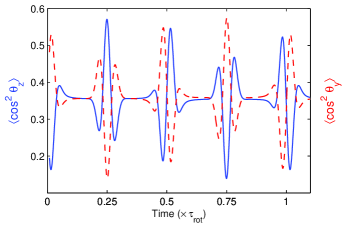
Figure 1: (Color online) Expectation values of the observables $\cos^{2}\theta_{z}$ (full line) and $\cos^{2}\theta_{y}$ (dashed line) for $a^{2}=1/3$, $\xi=11.1$ and $\tilde{T}=20$, as a function of normalized time.

To analyze the alignments along the two axes, in addition to $\langle\cos^{2}\theta_{z}\rangle(t)\equiv\langle\psi(\theta_{z},\phi_{z};t)|\cos^{2}\theta_{z}|\psi(\theta_{z},\phi_{z};t)\rangle$ one can consider the observable $\langle\cos^{2}\phi_{z}\rangle(t)\equiv\langle\psi(\theta_{z},\phi_{z};t)|\cos^{2}\phi_{z}|\psi(\theta_{z},\phi_{z};t)\rangle$, where $|\psi(\theta_{z},\phi_{z};t)\rangle$ is the state of the molecule given by the Schrödinger equation. However, it is more appropriate to introduce the observables $\langle\cos^{2}\theta_{x}\rangle(t)\equiv\langle\cos^{2}\phi_{z}\sin^{2}\theta_{z}\rangle(t)$ and $\langle\cos^{2}\theta_{y}\rangle(t)\equiv\langle\sin^{2}\phi_{z}\sin^{2}\theta_{z}\rangle(t)$, $\theta_{x}$ ($\theta_{y}$) corresponding to the polar angle with respect to the $x$-axis ($y$-axis). This is motivated by the fact that these observables are closely related to the experimental measurements and the fact that they will allow us to identify the ellipticity leading to quantitatively equivalent alignments along both the major axis ($x$ or $y$) of the polarization ellipse and the $z$-axis orthogonal to the ellipse. Because of the relation $\sum_{i=x,y,z}\langle\cos^{2}\theta_{i}\rangle(t)=1$, the alignment alternation can be measured with any pair of observables among $\{\langle\cos^{2}\theta_{i}\rangle(t),\ i=x,y,z\}$. Figure 1 displays the temporal behaviour of these thermally averaged quantities for an elliptically polarized field interacting with a molecule at the dimensionless temperature $\tilde{T}:=kT/B=20$ (an initial statistical ensemble of even values of $j$ is considered). This amounts to having $T=11$ K for a CO₂ molecule. Here $a^{2}=1/3$ and $\xi=11.1$ (corresponding approximately to a pulse of peak intensity $I=25\times 10^{12}$ W/cm² and of duration $\tau_{\text{FWHM}}=100$ fs for CO₂). During each rotational period $\tau_{\text{rot}}$ we can identify four revivals for both $\langle\cos^{2}\theta_{y}\rangle(t)$ and $\langle\cos^{2}\theta_{z}\rangle(t)$. The revivals occur around the times $t_{n}=n\tau_{\text{rot}}/4$ for both expectation values, as is the case for a linear polarization. The localization properties of the rotational wave packet are however fundamentally different. Near the highest peaks of $\langle\cos^{2}\theta_{z}\rangle(t)$ (at the times $t_{1}$, slightly after $t_{2}$ and also slightly before $t_{4}$), the molecule is predominantly aligned along the $z$-direction (small $\theta_{z}$), i. e. orthogonally to the polarization ellipse. This state is represented in spherical coordinates at time $t=t_{1}\equiv\tau_{\text{rot}}/4$ in Fig. 2 (left panel). At the highest peaks of $\langle\cos^{2}\theta_{y}\rangle(t)$ (slightly before $t_{2}$, at the time $t_{3}$ and also slightly after $t_{4}$), coinciding with the minima of $\langle\cos^{2}\theta_{z}\rangle(t)$, the molecule is aligned along the major axis (small $\theta_{y}$ and $\theta_{z}$ close to $\pi/2$). A representation of the molecular state is displayed at time $t=t_{3}\equiv 3\tau_{\text{rot}}/4$ in Fig. 2 (right panel).

As will be discussed below, the alignments revivals are quantitatively similar in both the $y$ and $z$-directions for the particular value $a^{2}=1/3$. The quantities $\langle\cos^{2}\theta_{z}\rangle(t)$ and $\langle\cos^{2}\theta_{y}\rangle(t)$ displayed in Fig. 1 are symmetric with respect to the approximate value 0.36, implying that $\langle\cos^{2}\theta_{x}\rangle(t)$ is close to 1/3 for all times. The angular distributions shown in Fig. 2 for $t=\tau_{\text{rot}}/4$ and $t=3\tau_{\text{rot}}/4$ are superposable upon rotation.

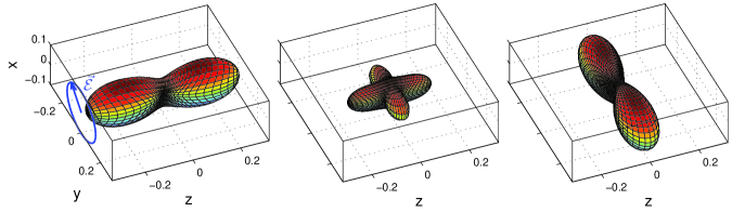
Figure 2: (Color online) Representation of the molecular state in spherical coordinates $\left\{r\equiv|\psi(\theta_{z},\phi_{z};t)|^{2},\theta_{z},\phi_{z}\right\}$ for $a^{2}=1/3$, $\xi=11.1$, $\tilde{T}=20$, at times $t=\tau_{\text{rot}}/4$ (left panel), $t\approx 3\tau_{\text{rot}}/8$ (middle panel) and $t=3\tau_{\text{rot}}/4$ (right panel). The polarization ellipse of the field $\vec{\mathcal{E}}$ is sketched in the $(x,y)$ plane.

Between the revivals, when the averaged observables are approximately flat as a function of time, locally near the times $t=(2p+1)\tau_{\text{rot}}/8$ (with integer $p$), it is remarkable that the state of the molecule is approximately an equal weight superposition of the two aligned states, as illustrated in Fig. 2 (middle panel). This can be interpreted as an extension of a recent proposal made in the linearly polarized case [13], where fractional revivals at odd multiples of $\tau_{\text{rot}}/8$ are shown to combine aligned (along the linear polarization axis) and antialigned (delocalized in the plane orthogonal to the axis) components with equal weights. In the current elliptic case, both components correspond to aligned states.

So far we have considered $a^{2}=1/3$. We now turn to the question of determining the value of this parameter giving an optimal two-direction alignment alternation, in the sense that both alignments correspond to similar (i. e. superposable upon rotation) delocalized angular distribution. Choosing $a=a_{\text{lin}}\equiv 0$ ($a=1$) gives a linear polarization along the $y$-axis ($x$-axis).

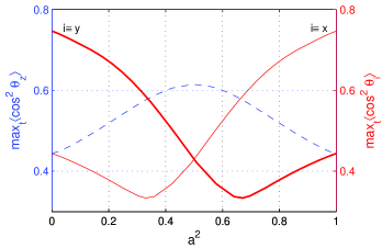
Figure 3: (Color online) Maximum over time of $\langle\cos^{2}\theta_{z}\rangle$ (dashed line), $\langle\cos^{2}\theta_{y}\rangle$ (full thick line), and $\langle\cos^{2}\theta_{x}\rangle$ (full thin line) with $\xi=11.1$ and $\tilde{T}=20$, as a function of $a^{2}$.

The circular polarization is obtained with $a^{2}=b^{2}=a_{\text{circ}}^{2}\equiv 1/2$. The optimal value is obtained when the maxima (over time) of both expectation values $\langle\cos^{2}\theta_{z}\rangle$ and $\langle\cos^{2}\theta_{y}\rangle$ for $a^{2}<1/2$ ($\langle\cos^{2}\theta_{x}\rangle$ for $a^{2}>1/2$) are equal. In Fig. 3 we plot these maxima as a function of $a^{2}$. The intersection points are near $a^{2}=1/3$ (corresponding to the ellipticity chosen for Figs 1 and 2) and $a^{2}=2/3$. This can be understood by rewriting the interaction term (3) in terms of the observable $\cos^{2}\theta_{y}$ rather than $\cos^{2}\phi_{z}$:

$$V_{\text{int}}=-\frac{\Delta\alpha}{4}\mathcal{E}^{2}(t)\left[(1-2a^{2})\cos^{2}\theta_{y}+a^{2}\sin^{2}\theta_{z}\right].$$ (5)

When the ellipticity is chosen such that $1-2a^{2}=a^{2}$, i.e. $a^{2}=1/3$, the directions $\theta_{y}$ and $\theta_{z}$ play a symmetric role. Notice from (5) that the minima in one direction correspond to the maxima in the other direction. In the sudden regime, both types of extrema are visited equivalenty in contrast to the adiabatic case. The ellipticity $a^{2}=1/3$ can be interpreted as the best compromise between linear and circular polarizations with the remarkable feature that the angular distribution associated with the highest revivals are similar in both directions (see Fig. 2). It is worth noting that this value is not the arithmetic average of $a_{\text{circ}}^{2}$ and $a_{\text{lin}}^{2}$. The case $a^{2}=2/3$ involves the direction $\theta_{x}$ instead of $\theta_{y}$. In Fig. 3 we also recognize the case of a circular polarization for $a^{2}=1/2$ where the alignment along $z$ is large whereas the maxima of $\langle\cos^{2}\theta_{x}\rangle$ and $\langle\cos^{2}\theta_{y}\rangle$ are equal, reflecting the fact that the rotational wavepacket is delocalized for all times in the $x,y$-plane.

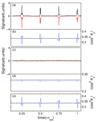
Figure 4: (Color online) Field-free alignment of an ensemble of CO₂ molecules ($T=296$ K, $P=4\times 10^{4}$ Pa) produced by an elliptically polarized pump field [$a^{2}\approx 1/3$, see Eq. (1)] of peak intensity 25 TW/cm² and pulse duration $\tau_{\text{FWHM}}=100$ fs. Cross defocusing signal recorded as function of delay with the probe field linearly polarized along (a) the $y$-axis (major field axis) and (c) the $x$-axis (minor field axis). In (a) and (c), the theoretical results (thick lines) are shown as mirror images of the experimental ones. Corresponding observables (b) $\langle\cos^{2}\theta_{y}\rangle$ and (d) $\langle\cos^{2}\theta_{x}\rangle$. (e) $\langle\cos^{2}\theta_{z}\rangle$ along the propagation $z$-axis deduced from (b) and (d). The isotropic values 1/3 are indicated with dashed lines.

We have demonstrated the effect experimentally in CO₂ molecules at room temperature by measuring the optical Kerr effect along the two orthogonal directions, $x$ and $y$ respectively (both orthogonal to the $z$-direction of propagation of the beam). The measurements have been performed with a Ti:sapphire chirped-pulse amplifier producing 100-fs pulses at 1 kHz. Recently it has been shown [14] that measuring the defocusing of a time-delayed weak probe pulse produced by a spatial distribution of aligned linear molecules yields a signal proportional to $(\langle\cos^{2}\theta\rangle(t)-1/3)^{2}$, with $\theta$ the angle between the molecular axis and the direction of the probe field. Choosing the polarization of the probe either in the $y$ or $x$-direction, we can thus obtain $[\langle\cos^{2}\theta_{i}\rangle(t)-1/3]^{2}$ (shown in Fig. 4a,c), where $\theta_{i}$ is the angle between the molecular axis and the $i$-axis ($i=x,y$). From these we can deduce $\langle\cos^{2}\theta_{y}\rangle$ and $\langle\cos^{2}\theta_{x}\rangle$ which characterize the alignment along the major and minor axes of the ellipse, respectively (Fig. 4b, d). The shape and amplitude of the recorded signal are in good agreement with the theoretical predictions. The quasi-isotropic feature of the alignment along the $x$-axis mentioned above for this specific ellipticity is confirmed by this experiment, where a signal close to zero is observed in Fig. 4c. The alignment along the $z$-axis , characterized by $\langle\cos^{2}\theta_{z}\rangle(t)$ (Fig. 4e), can be deduced from the other two observables through the relation $\sum_{i=x,y,z}\langle\cos^{2}\theta_{i}\rangle(t)=1$. The results of Fig. 4b and e show clearly the experimental alternation of the alignment predicted theoretically and represented in Fig. 1. It should be noted that the experimental signal related to the measurement of $(\langle\cos^{2}\theta_{x}\rangle(t)-1/3)^{2}$ is found to be minimum for the ellipticity $a^{2}=1/3$, as predicted by the model. As discussed above, the fact that $\langle\cos^{2}\theta_{x}\rangle(t)\approx 1/3$ (in a strong field) is a clearcut signature of optimal alignments in the two other directions. An exhaustive experimental investigation with other ellipticities has been performed and shows strong modifications of both shape and amplitude of the recorded signals, in agreement with numerical simulations.

In conclusion, we have shown, both theoretically and experimentally, that a linear molecule subjected to a short specific elliptically polarized laser field can be aligned, alternatively, at specific times along the orthogonal axis and the major axis of the ellipse. Contrary to the adiabatic case where only the minima of the induced potential are populated, for short pulses all the extrema of the potential are dynamically visited and appear as revivals. The control of this field-free two-direction alignment alternation is a challenging perspective that could find applications in nano-technology, for instance to generate a 3D molecular switch [1]. In the context of quantum information, the advantage of an elliptic polarization over a linearly polarized field employed in a recent proposal [15] is to have a superposition of alignments along two axes, instead of a superposition of an alignment and a planar delocalization.

This research was supported by the Conseil Régional de Bourgogne, the Action Concertée Incitative Photonique from the French Ministry of Research, and a Marie Curie European Reintegration Grant within the 6th European Community RTD Framework Programme.

References

- [1] H. Stapelfeldt and T. Seideman, Rev. Mod. Phys. 75, 543 (2003).
- [2] J. J. Larsen, K. Hald, N. Bjerre, H. Stapelfeldt and T. Seideman, Phys. Rev. Lett. 85, 2470 (2000).
- [3] J. Karczmarek, J. Wright, P. B. Corkum and M. Ivanov, Phys. Rev. Lett. 82, 3420 (1999).
- [4] D. M. Villeneuve, S. A. Aseyev, P. Dietrich, M. Spanner, M. Y. Ivanov, and P. B. Corkum, Phys. Rev. Lett. 85, 542 (2000).
- [5] M. Spanner, K. M. Davitt, and M. Y. Ivanov, J. Chem. Phys. 115, 8403 (2001).
- [6] N. V. Vitanov and B. Girard, Phys. Rev. A 69, 033409 (2004).
- [7] F. Rosca-Pruna and M. J. J. Vrakking Phys. Rev. Lett. 87, 153902 (2001); F. Rosca-Pruna and M. J. J. Vrakking, J. Chem. Phys. 116, 6567 (2002); F. Rosca-Pruna and M. J. J. Vrakking, J. Chem. Phys. 116, 6579 (2002).
- [8] V. Renard, M. Renard, S. Guérin, Y. T. Pashayan, B. Lavorel, O. Faucher, and H. R. Jauslin Phys. Rev. Lett. 90, 153601 (2003); V. Renard, M. Renard, A. Rouzée, S. Guérin, H. R. Jauslin, B. Lavorel, and O. Faucher Phys. Rev. A 70, 033420 (2004).
- [9] B. Friedrich and D. Herschbach, Phys. Rev. Lett. 74, 4623 (1995).
- [10] A. Keller, C. M. Dion and O. Atabek, Phys. Rev. A 61, 023409 (2000).
- [11] N. E. Henriksen, Chem. Phys. Lett. 312, 196 (1999).
- [12] D. Daems, S. Guérin, H. R. Jauslin, A. Keller and O. Atabek, Phys. Rev. A 69, 033411 (2004).
- [13] M. Spanner, E. A. Shapiro, and M. Ivanov, Phys. Rev. Lett. 92, 093001 (2004).
- [14] V. Renard, O. Faucher, and B. Lavorel, Opt. Lett. 30, 70 (2005).
- [15] K. F. Lee, D. M. Villeneuve, P. B. Corkum, and E. A. Shapiro Phys. Rev. Lett. 93, 233601 (2004).