Binomial states and the phase distribution measurement of weak optical fields

Abstract

We show that the eight-port interferometer used by Noh, Fougères, and Mandel [Phys. Rev. Lett. 71, 2579 (1993)] to measure their operational phase distribution of light can also be used to measure the canonical phase distribution of weak optical fields, where canonical phase is defined as the complement of photon number. A binomial reference state is required for this purpose, which we show can be obtained to an excellent degree of approximation from a suitably squeezed state. The proposed method requires only photodetectors that can distinguish among zero, one and more than one photons and is not particularly sensitive to photodetector imperfections.

I Introduction

The quantum mechanical nature of the phase of light has been studied since the beginnings of quantum electrodynamic theory Dirac , with renewed interest recently. The study of quantum phase is distinguished from the study of many other quantum observables by the difficulties inherent not only in finding a theoretical description but also in finding methods for measuring the phase observable so described Bibliog . A method of circumventing this latter difficulty is to define phase as the quantity measured by some particular experiment. This is known as an operational approach B and D . A sensible operational phase measurement must, of course, be in accord with a classical phase measurement in the appropriate limit, for example when the field being measured is in a strong coherent state. This requirement, however, is not sufficient to define a unique operational phase observable and various different operational definitions have been proposed. The best known of these is that of Noh et al. Mandel who also proposed a means of measuring an operational phase distribution Mandel2 , which was further developed in Refs Mandel3 and Mandel4 . There are also various theoretical approaches to describing the phase observable. What distinguishes these theoretical approaches from one another is their predicted phase distributions for particular states. Some of these approaches are motivated by the aim of expressing phase as the complement of photon number, in the spirit of Dirac’s original work Dirac . Examples of such approaches include the probability operator measure approach Hel , a formalism in which the Hilbert space is doubled Newton , a limiting approach based on a finite Hilbert space PB and a more general axiomatic approach Ulf . Although these particular approaches are quite distinct they all lead to the same phase probability distribution for a field in state $\left|\psi\right\rangle$ as a function of phase angle $\theta$ Ulf :

$$P(\theta)=\frac{1}{2\pi}\left|\sum_{n=0}^{\infty}\left\langle\psi|n\right\rangle\exp(in\theta)\right|^{2}$$ (1)

where $\left|n\right\rangle$ is a photon number state. Leonhardt et al. Ulf have called this the “canonical” phase distribution to indicate a quantity that is the canonical conjugate, or complement, of photon number. Irrespective of how it is derived, the canonical phase distribution has properties that one might expect from the complement of photon number: it is shifted uniformly when a phase shifter is applied to the field, it is not changed by a photon number shift Ulf and it corresponds to a wavefunction in the phase representation of which the photon number amplitude is the finite Fourier transform Bibliog ; Conj . The last property is a natural parallel to momentum-position conjugacy.

Although the canonical phase distribution has attractive theoretical properties, its direct measurement presents difficulties Footnote . Good approximate methods exist, based on homodyne techniques, for measuring the canonical phase distribution of states with narrow phase distributions, for example coherent states with mean photon numbers of at least five VandP . Weak fields in the quantum regime, however, must have broad phase distributions because of number-phase complementarity. In principle the distributions for such fields can be measured by the projection synthesis method proposed in Ref. Proj Syn but this requires the generation of a reciprocal binomial state as a reference state. The generation of this exotic state has still not been achieved. On the other hand the operational phase measurements of Noh et al. are quite practical for the weak fields of interest and have been shown to measure what they are designed to measure very well Mandel2 . Unfortunately they were not designed to measure, nor do they measure, the canonical phase distribution. Indeed their results show that their operational phase distribution is significantly different from the canonical phase distribution. Thus the projection synthesis method measures the canonical phase distribution in principle while the operational method does not; but the operational method is practical while the projection synthesis method is not.

In this paper we show how the apparatus used for measuring the operational phase distribution can be used to measure the canonical phase distribution for weak fields in conjunction with a reference field in a binomial state. We show how a binomial state, in contrast to a reciprocal binomial state, can be very well approximated by a squeezed state, making this method much more practical than the original projection synthesis method.

II projection synthesis

II.1 Beam splitter

In the projection synthesis method of Proj Syn the aim was to use photodetection in conjunction with a beam splitter and a special reference state to synthesize the projection of an unknown state onto a truncated phase state

$$\left|\theta\right\rangle=\frac{1}{(M+1)^{1/2}}\sum_{n=0}^{M}\exp(in\theta)\left|n\right\rangle$$ (2)

where $M$ must be sufficiently large for the density matrix of the reproducible weak field that is to be measured to be well approximated in the number state basis by a matrix with only the first $(M+1)\times(M+1)$ elements non-zero. This projection event is associated with the detection of $M$ photons in one output mode of the beam splitter and no photons in the other. We label this detection event $(M,0)$. The probability of the event $(M,0)$ is obtained from the occurrence frequency in successive repeated measurements of the field. The procedure is to measure this probability as $\theta$ is changed in small steps over the $2\pi$ range. The changes in $\theta$ can be achieved simply by altering the phase either of the reference field or of the field to be measured. A histogram is then plotted which, when suitably normalized, produces the canonical phase distribution.

The mechanism underlying projection synthesis can be described as follows. Suppose the measured and reference fields are in the beam splitter input modes $0$ and $1$ respectively and the event $(M,0)$ is that for which $M$ photons are detected in output mode $0$ and zero photons are detected in output mode $1$. The combined output state corresponding to this measurement result is the $M$-photon state $\left|M\right\rangle_{0}\left|0\right\rangle_{1}$. Following the unitary evolution of this state backwards through the beam splitter transforms this to an $M$-photon entangled input state of the form

$$\left|f\right\rangle=\sum_{n=0}^{M}f_{m}\left|n\right\rangle_{0}\left|M-n\right\rangle_{1}$$ (3)

which displays photon number conservation. If the measured field is in a pure state $\left|\psi\right\rangle_{0}$ and the reference state is given by

$$\left|r\right\rangle_{1}=\sum_{n=0}^{\infty}r_{n}\left|n\right\rangle_{1}$$ (4)

then the amplitude for the detection event $(M,0)$ is ${}_{0}\langle\psi|\,_{1}\langle r|f\rangle$, that is, the projection of $|\psi\rangle_{0}$ onto ${}_{1}\langle r|f\rangle$. By choosing appropriate coefficients $r_{n}$ for $n=0$ to $M$, we can make this amplitude proportional to the projection of $\left|\psi\right\rangle_{0}$ onto the truncated phase state $\left|\theta\right\rangle$ given by (2). We note that the values of $r_{n}$ for $n>M$ are irrelevant, merely affecting the normalization factor for the complete probability distribution. For a 50:50 symmetric beam splitter we find that the values of $\left|r_{n}\right|$ need to be proportional to the reciprocal of the square root of the binomial coefficient ${M\choose n}$ for $n=0$ to $M$.

As mentioned earlier, the difficulty with projection synthesis is generating the reciprocal binomial state required for the reference field. As reciprocal binomial states have a finite number of photon number state coefficients, they can be prepared as travelling fields in principle by the generic methods given in Refs. Generation and Dakna by means of beam splitters. Unfortunately, however, in such techniques the state generated is conditioned on measuring particular outputs from the beam splitters and so the method is quite inefficient and difficult and has never been implemented.

II.2 Multiport device

Projection synthesis relies on transforming projections onto photon number states into at least one projection onto a truncated phase state. As phase is not an absolute quantity, it is necessary to have a transformation device with at least two inputs for phase measurement: one for the field to be measured and one for the reference field. The projection synthesis method of Proj Syn uses the minimal necessary device, a beam splitter with two inputs and two outputs. More flexibility can be obtained by using a more general multiport device with $N+1$ inputs and $N+1$ outputs with a photodetector in each output. This would require, in addition to the field in state $|\psi\rangle_{0}$ to be measured being in input mode $0$, say, $N$ reference fields being in modes 1,2 $\ldots N$. Rather than exacerbate the problem of preparing special reference states, it is preferable simply to have one reference field in input mode 1 with vacuum fields in the remaining inputs. These input states are transformed by a unitary operator $\widehat{R}$ into the output states. If a total of $M$ photons are detected in the output states then, from photon number conservation, the corresponding $M$-photon output state evolved backwards through the multiport device will be transformed to an entangled $M$-photon input state. Projecting the combined vacuum input state $\left|0\right\rangle_{2}\left|0\right\rangle_{3}\ldots\left|0\right\rangle_{N}$ onto this entangled state will result in a two-mode $M$-photon entangled state in input modes $0$ and $1$ of the form $\left|f\right\rangle$ in (3). The coefficients $f_{m}$ will depend on the unitary transformation $\widehat{R}$ and on the manner in which the $M$ photons are detected, that is, how they are distributed over the output modes. As these coefficients determine the values of $r_{n}$ required to synthesize the projection of the state to be measured onto a truncated phase state, use of a multiport device should increase the flexibility in choosing a convenient reference state $|r\rangle_{1}$.

A natural multiport extension of the 50:50 symmetric beam splitter is one where $\widehat{R}$ is such that a photon entering any input appears with equal probability at any output Mattle ; Torma and a photon in any output is equally likely to have come from any input. In this case it is not difficult to show that, when the $M$ photons are detected in output mode $0$ and none are detected in the other modes, the coefficients $f_{m}$ are similar to those for the beam splitter case for the event $(M,0)$ and we again require the reference field to be in a reciprocal binomial state. Thus it is worth examining other possible distributions of the detected photons over the output modes.

A particular case of the above device is one that performs a discrete Fourier transform Torma , that is where the set of mode photon creation operators and the set of transformed operators form a discrete Fourier transform pair:

$$\widehat{R}^{\dagger}\widehat{a}_{j}^{\dagger}\widehat{R}=\sum_{i=0}^{N}U_{ij}\widehat{a}_{i}^{\dagger}$$ (5)

$$\widehat{a}_{i}^{\dagger}=\sum_{j=0}^{N}U_{ij}^{*}\widehat{R}^{\dagger}\widehat{a}_{j}^{\dagger}\widehat{R}$$ (6)

where

$$U_{ij}=\frac{\omega^{ij}}{\sqrt{N+1}}$$ (7)

with $\omega=\exp[-i2\pi/(N+1)]$, that is, a $(N+1)$th root of unity. Recently PregPRL , we found that, if the number $M$ of photons detected is equal to $N$ and these photons are distributed such that one is detected in each output of such a multiport device except one, then projection onto a truncated phase state is synthesized providing the reference field is in a binomial state. Specifically, if the detection event is such that it is the $m$th output detector that records a zero count while all the other detectors record one count each, then the state $|\psi\rangle_{0}$ to be measured is projected onto a state proportional to

$$\left|\theta_{m}\right\rangle_{0}=\sum_{n=0}^{N}U_{mn}^{*}\left|n\right\rangle_{0}$$ (8)

that is

$$\left|\theta_{m}\right\rangle_{0}=\frac{1}{(N+1)^{1/2}}\sum_{n=0}^{N}\exp(in\theta_{m})\left|n\right\rangle_{0}$$ (9)

where

$$\theta_{m}=m2\pi/(N+1)$$ (10)

which is just the required truncated phase state. The amplitude for this detection event is proportional to ${}_{0}\langle\theta_{m}|\psi\rangle_{0}$ PregPRL .

In addition to requiring photodetectors that only need to distinguish among zero photons, one photon and more than one photon, this multiport device has the advantage that the required binomial reference state is much closer to commonly available states such as coherent states than is a reciprocal binomial state. Binomial states have been studied for some time Stoler . They have interesting properties such as interpolating between coherent states and number states and, with the photon number state coefficients positive, they are partial phase states with a mean phase of zero Vid . It is not difficult to show that they have a smaller phase variance than truncated phase states with the same number of number state coefficients. As binomial states have a finite number of photon number state coefficients, they can be prepared as travelling fields by the generic methods given in Refs. Generation and Dakna by means of beam splitters. Unfortunately, however, these inefficient techniques offer no real advance when used for measuring the phase distribution over the use of a reciprocal binomial state in Proj Syn , which can be prepared by the same generic means. For a practical experiment we require the binomial state to be approximated by a state which is reasonably straightforward to prepare on demand.

As mentioned earlier, the values $r_{n}$ of the number state coefficients of the reference state for $n>M$ are irrelevant so here, where $M=N$, only the coefficients $r_{n}$ with $0\leq n\leq N$ are important, and thus only these need to be proportional to square roots of binomial coefficients. Further, as we are interested in fields with broad phase distributions, and states with broad number state distributions tend to have narrow phase distributions, then normally only a small group of number state coefficients ${}_{0}\langle n|\psi\rangle_{0}$ of the state of the measured field will differ significantly from zero. From (3) with $M=N$ and (4), if the coefficient ${}_{0}\langle n|\psi\rangle_{0}$ is significant then the value of $r_{N-n}$ is important. Thus, for example, if ${}_{0}\langle n|\psi\rangle_{0}$ are significant only for a small number of values of $n$ equal to or slightly less than a value $n^{\prime}$, say, then we would choose $N=n^{\prime}$ and require the small number of coefficients $r_{n}$ with $n$ equal to, or near, zero to be proportional to square roots of appropriate binomial coefficients. We show in the Appendix how such a state can be approximated by a squeezed state with squeezing parameter $\tanh^{-1}0.5$. On the other hand if the significant values of ${}_{0}\langle n|\psi\rangle_{0}$ occur for $n$ equal to or near zero, as will be the case for very weak fields, then we require coefficients $r_{n}$ with $n$ equal to or slightly less $N$ to be proportional to square roots of the appropriate binomial coefficients. In the Appendix we find a squeezed state, also with squeezing parameter of $\tanh^{-1}0.5$, that is a very good approximation for the binomial reference state needed for measuring the phase distribution of very weak fields with the eight-port interferometer examined below.

III Eight-port interferometer

III.1 Binomial reference state

The eight-port interferometer Walker used by Noh et al. Mandel ; Mandel2  and Torgerson and Mandel Mandel2 ; Mandel3 is illustrated in Fig. 1. There are four 50:50 symmetric beam splitters at the corners of a square. The phase shifter labelled $-i$ between the two beam splitters on the right shifts the phase by $\pi/2$. The field state $|\psi\rangle_{0}$ to be measured is in input port 0. The phase shifter in input port $1$ allows the phase of the reference field state $|r\rangle_{1}$ to be changed. The dotted phase shifters in input port $2$ and before detectors D₁, D₂ and D₃, which are not present in the original interferometer, are merely inserted here for mathematical convenience. As the field in input port 2 is the vacuum it will not be affected by a phase shift and, as the detectors detect photons, their operation will not be affected by phase shifters in front of them.

Figure 1: Eight-port interferometer for measuring the canonical phase distribution of weak fields. The field in state $|\psi\rangle_{0}$ to be measured is in the input port labelled In 0, the reference field in state $|r\rangle_{1}$ is in input port In 1 and vacuum state fields are in In 2 and In 3. A photodetector is in each output port. The dotted phase shifters are for mathematical convenience only, and do not affect the results.

A single 50:50 symmetric beam splitter transforms the input creation operators $\widehat{b}^{\dagger}$ and $\widehat{c}^{\dagger}$ in accord with Book

$$\widehat{R}_{1}\widehat{b}^{\dagger}\widehat{R}_{1}^{\dagger}=2^{-1/2}(\widehat{b}^{\dagger}+i\widehat{c}^{\dagger})$$ (11)

$$\widehat{R}_{1}\widehat{c}^{\dagger}\widehat{R}_{1}^{\dagger}=2^{-1/2}(\widehat{ib}^{\dagger}+\widehat{c}^{\dagger})$$ (12)

where $\widehat{R}_{1}$ is the unitary operator for the action of the single beam splitter. By using this relation successively, it is not difficult to show that the input creation operators for the eight-port interferometer, including the dotted phase shifters, are transformed as

$$\widehat{R}\widehat{a}_{i}^{\dagger}\widehat{R}^{\dagger}=\exp(i\gamma)\sum_{i=0}^{3}U_{ij}^{*}\widehat{a}_{j}^{\dagger}$$ (13)

where

$$U_{ij}=\frac{\omega^{ij}}{2}$$ (14)

with $\omega$ again being $\exp[-i2\pi/(N+1)]$, provided we set the phase shifter in input $1$ to shift the phase by $\pi/2$, that is to attach a value $-i$ to it. Expressions (13) and (14) are in agreement with (6) and (7) for $N=3$ apart from the phase factor $\exp(i\gamma)$, which depends on the difference between the distance between beam splitters and an integer number of wavelengths. This phase factor does not affect the photocount probabilities and can be ignored.

Thus we see that the eight-port interferometer, without modification, can be used to synthesize the projection of the state to be measured onto one of four phase states. Specifically the probability of measurement event (0, 1, 1, 1), that is the detection of zero photocounts in detector D₀ and one in each of D₁, D₂ and D₃, is proportional to the square of the modulus of the projection of the measured state onto the truncated phase state

$$\left|\theta_{0}\right\rangle=2^{-1}(\left|0\right\rangle+\left|1\right\rangle+\left|2\right\rangle+\left|3\right\rangle)$$ (15)

while the probability of the event (1,0,1,1) is proportional the square of the modulus of the projection of the measured state onto the truncated phase state

$$\left|\theta_{1}\right\rangle=2^{-1}(\left|0\right\rangle+i\left|1\right\rangle-\left|2\right\rangle-i\left|3\right\rangle)$$ (16)

and so on, in accord with (9) with $N=3$. Repeating the experiment a number of times with a reproducible state will allow a probability $P_{M}(\theta_{m})$ with $m=0,1,2,3$ to be measured for each of the four events (0,1,1,1), (1,0,1,1), (1,1,0,1) and (1,1,1,0) respectively.

To use these four measured probabilities to construct the phase distribution we first normalize them to

$$y(\theta_{m})=\frac{2P_{M}(\theta_{m})}{\pi\sum_{m}P_{M}(\theta_{m})}.$$ (17)

We note that, as shown in general in Ref. PregPRL , $P_{M}(\theta_{m})\propto|\langle\psi|\theta_{m}\rangle|^{2}$, where here $|\theta_{m}\rangle$ is given by (9) with $N=3$ and we have omitted the subscripts zero for convenience. This allows us to replace $P_{M}(\theta_{m})$ in (17) by $|\langle\psi|\theta_{m}\rangle|^{2}$. Substituting for $\theta_{m}$ from Eq. (10) with $N=3$ yields eventually

$$\sum_{m=0}^{3}|\langle\psi|\theta_{m}\rangle|^{2}=|\langle\psi|0\rangle|^{2}+|\langle\psi|1\rangle|^{2}+|\langle\psi|2\rangle|^{2}+|\langle\psi|3\rangle|^{2}.$$ (18)

If the measured field is sufficiently weak for the number state components $\left\langle\psi|n\right\rangle$ to be negligible for $n\geq 4$ then the right-hand side of Eq. (18) is just unity and so, from (17),

$$y(\theta_{m}) = \frac{2}{\pi}|\langle\psi|\theta_{m}\rangle|^{2}$$ (19)

$$= P(\theta_{m}),$$

with the last line being obtained from Eq. (1) in the same weak-field approximation.

Thus, if we normalize the four measured probabilities by dividing each by the sum of the four and then multiplying by $2/\pi$, we obtain four points on the canonical phase probability distribution given by Eq. (1) for a weak field. We note that, with this normalization procedure, if the points $y(\theta_{m})$ are used to draw a histogram, the area of the histogram would unity, because the width of each rectangle is $\pi/2$.

Shifting the phase of the phase shifter in the input $1$ to change the phase of the reference field by $\Delta\theta$ and repeating the procedure gives four more points of the distribution shifted from the original points by $\Delta\theta$. A sixteen point curve, for example, can be constructed by shifting the phase by $\pi/8$ three times and repeating the experiment after each shift.

III.2 Squeezed reference state

The above analysis and suggested procedure assumes that the reference field is in a perfect binomial state. If, instead, we use the squeezed state approximation to the binomial state as derived in the Appendix, then the vacuum state coefficient differs from the ideal value and the measured state is no longer projected onto the truncated phase state $\left|\theta_{m}\right\rangle$ but is instead projected onto a state proportional to

$$|0\rangle+\exp(i\theta_{m})|1\rangle+\exp(2i\theta_{m})|2\rangle+1.0146\exp(3i\theta_{m})|3\rangle.$$ (20)

We would expect that this would lead to some small errors when the procedure suggested above is applied. In practice, if we are measuring a state, such as a coherent or squeezed state, that does not have a truncated photon number distribution, the error caused by the modulus of the three-photon coefficient in expression (20) differing from unity may in general be smaller that the error caused by the truncation of expression (20) after the three-photon component. In Fig. 2 we show the points obtained from a simulated experiment for a coherent state with a mean photon number of 0.076, which is is comparable to the field strength of interest in Ref. Mandel3 , using a squeezed reference state. The close agreement with the canonical distribution is apparent. For weaker fields, for example the other field of interest in Ref. Mandel3 with a mean photon number of 0.047, the agreement is even closer. Agreement is still good for stronger coherent state fields with mean photon numbers of 0.139 and 0.23, as used in Ref. Mandel4 , with divergence from the canonical distribution becoming apparent for mean photon numbers of around 0.4. Figure 3 shows simulated results for a coherent state with a mean photon number of 0.5. The error here is almost entirely due to the truncation of the phase state rather than to the non-unit coefficient of the fourth term in (20). A mean photon number of 0.5 represents the approximate limit to the field strength for a coherent state for which this measurement technique is suitable.

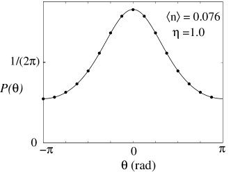
Figure 2: Canonical phase probability distribution $P(\theta)$ for a coherent state field with a mean photon number of 0.076. The full line is the theoretical result and the dots are simulated measured results with ideal detectors for four different phase settings of the squeezed reference field.

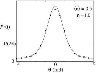
Figure 3: Simulated measurements (dots) and the theoretical canonical phase distribution (full line) for a coherent state field with a mean photon number of 0.5 with ideal detectors.

IV Some practical considerations

To obtain an idea of the number of experiments needed to measure the required probabilities, we note that, for weak coherent fields of the strengths discussed here, the coefficient of the vacuum component dominates, so the probability of detecting a total of three photons will be approximately the probability that the binomial reference state contains three photons, which is 12.5%. These photons can be detected as a variety of events such as (0,1,1,1), (0,0,2,1) or (0,0,0,3). The fraction of these events that are required events, that is three separate counts of one photon and one count of zero, is 3/32. Thus approximately 4.7% of experiments will produce one of the four desired events. After running the experiment sufficient times to obtain the four probabilities with the desired accuracy, the phase of the reference state is then changed and the procedure is repeated to obtain four more probabilities. The question therefore arises: how many probabilities, that is points on the probability distribution, do we need to determine the distribution with reasonable accuracy? The fact that we are synthesizing a projection onto a truncated phase state with four non-zero photon number-state coefficients means that the weak fields being measured must, by necessity, have negligible coefficients for components with photon numbers greater than three. From Eq. (1) this means that the most rapidly oscillating Fourier component of the distribution $P(\theta)$ behaves as $\exp(i3\theta)$. To detect this oscillation we would need a minimum of about 12 equally spaced values of $P(\theta)$. Thus running the experiment with four different phase settings, giving a total of 16 points on the distribution curve as shown in Fig. 2, should normally be sufficient.

In a practical experimental situation errors can arise from collection inefficiencies, non-unit quantum efficiencies for one, two and multiple photon detection, dead times and accidental counts arising from dark counts and background light. The fact, however, that Noh et al. Mandel have performed successful experiments involving the measurement of joint detection probabilities with an eight-port interferometer, by means of photon counting, for states with field strengths similar to those of interest in this paper is an encouraging indication that there should be no insurmountable difficulties for the method proposed here arising from such errors. It is worth considering some specific aspects of the sources of error. In the experiments of Noh et al. Mandel photon count rates were of the order of $10^{4}$ per second with a counting interval of about 5 $\mu$s, to give the required small mean photon number, and dead-time effects were negligible. In the present proposed experiment dead times are even less important because it is only necessary to discriminate among zero, one and many counts rather than among general numbers of counts Paul . Dark counts can be reduced to about 200 per second Mandel or even to 20 per second Trif by cooling the detectors and background light can be reduced by appropriate shielding. In the event that the residual dark and background counts are not negligible, the measured joint probabilities of the four photocount events can be corrected by a deconvolution procedure using the data obtained by blocking the input signals Mandel .

Concerning detector efficiencies, even if collection efficiencies are made to approach unity by, for example, suitable geometry and reflection control, there will still be some detector inefficiency due to non-unit quantum efficiency, so some correction for detector inefficiency may be needed. Conventional single-photon counting module detectors can have an efficiency of around 0.7 Tak , while visible light photon counters that distinguish between single-photon and two-photon incidence can have quantum efficiencies of about 0.9 with some sacrifice of smallness of dark count rate Tak . We denote the one-photon detection efficiency, that is the probability of recording one photocount if one photon is present, by $\eta$. Then, as dead times are not important, the general multiple detection efficiency is such that the probability of recording $n$ photocounts if $N$ photons are present is ${N\choose n}\eta^{n}(1-\eta)^{N-n}$ where the first factor is the binomial coefficient Lee . If $\eta$ is the same for all four detectors the probability for the joint four-count detection event $(m,n,p,q)$ is given by

$$P_{c}(m,n,p,q)=\sum_{s=m}^{\infty}\sum_{t=n}^{\infty}\sum_{u=p}^{\infty}\sum_{v=q}^{\infty}{s\choose m}{t\choose n}{u\choose p}{v\choose q}$$

$$\times\eta^{m+n+p+q}(1-\eta)^{s+t+u+v-m-n-p-q}P_{I}(s,t,u,v)$$ (21)

where $P_{I}(s,t,u,v)$ is the probability that an ideal detector would have detected the joint four-count event $(s,t,u,v)$. The relation (21) can be inverted by use of the four-function Bernoulli transform, which is straightforward to derive in a similar manner to that of the two-function transform derived in Ref. PeB . This allows us to calculate the ideal probabilities from the measured probabilities and thus correct for non-unit efficiencies.

Although we can correct for non-unit efficiencies an analysis shows that the effect of not correcting for them is not as serious as it may first appear. Essentially this is because the four measured probabilities are always normalized so their sum is $2/\pi$. The major effect of $\eta$ not being unity is, as can be seen from (21), that the probabilities for the four events (0,1,1,1), (1,0,1,1), (1,1,0,1) and (1,1,1,0) to be actually recorded are reduced by a factor $\eta^{3}$. As this affects the event probabilities uniformly, however, the effect vanishes upon normalization. The next order effect is that some ideal four-count events, such as (1,1,1,1) and (0,2,1,1), are registered, for example, as (0,1,1,1) because of the inefficiency. The effect of this is only partially removed by the normalization. Ideal higher-count events also contribute to the error, but for weak fields the probability of ideal high-count events is not large. A numerical calculation of the total effect of non-unit efficiency, including the effect of normalization, shows that the proposed procedure is not highly sensitive to detector inefficiency, provided the efficiency is reasonable, for the weak states of interest. More precisely, for coherent states with a mean photon number up to 0.5 photons, as discussed above, the error in the final normalized probabilities is less than 2% for $\eta\geq 0.9$. For a mean photon number of 0.076, the error is less that 0.5% for such efficiencies. In Fig. 4 we show the effect of a poorer efficiency of $\eta=0.6$ for a mean photon number of 0.076.

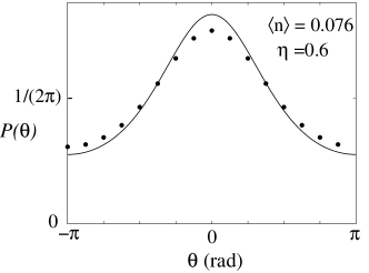
Figure 4: Uncorrected simulated measurements (dots) and the theoretical canonical phase distribution (full line) for a coherent state field with a mean photon number of 0.076 where the photodetectors have an efficiency $\eta=0.6$.

To produce the squeezed state required as an approximate binomial state, we note that squeezed vacuum states can be transformed into various types of squeezed states, the squeezing axis can be rotated, coherent amplitude can be added and the squeezing can be controlled independently of the coherent amplitude. The degree of squeezing needed here is of a magnitude that is a realistic expectation either now or in the near future Bachor .

Our discussion has focused mainly on measuring the phase probability distribution of pure states of light. It is straightforward, however, to show that our procedure can also be used to measure the distribution of a mixed state. If the mixed state is represented by a density operator that is a weighted sum of pure state density operators $|\psi\rangle\langle\psi|$ for various states $|\psi\rangle$, then the phase probability density is just the corresponding weighted sum of values of $P(\theta)$ given expression (1) for the various states $|\psi\rangle$. To measure this, we can use precisely the same procedure as described in this paper with the same binomial reference state.

V conclusion

We have shown in this paper how the eight-port interferometer used by Noh et al. Mandel ; Mandel2 to measure their operational phase distribution can used to measure the canonical phase distribution given by Eq. (1), where the canonical phase is defined as the complement of photon number. The procedure is applicable for weak fields in the quantum regime, by which we mean explicitly states for which number state components for photon numbers greater than three are negligible. For coherent states, this requirement translates to a mean photon number of a half a photon or less. This is precisely the quantum regime in which large differences between the operational phase and the canonical phase distributions are most apparent. For example fields of interest in Refs Mandel3 ; Mandel4 are coherent states with mean photon numbers of 0.23, 0.139, 0.076 and 0.047. The success of the experiments in the foregoing references indicates that the procedure proposed in this paper should be viable, given a reliable source of the required reference state.

The procedure in this paper has advantages over the original projection synthesis method proposed for measuring the canonical phase distribution. The most significant of these is that the present procedure requires a binomial reference state rather than a reciprocal binomial state. We have shown that the required binomial state can be approximated by a squeezed state sufficiently well for our purpose. Another advantage is that we require only photodetectors that can distinguish among zero, one and more than one photocounts. The measurements are not particularly sensitive to photodetector inefficiency and, for reasonably good detector efficiencies, no corrections should be needed. Overall, we feel that the proposal in this paper brings the measurement of the canonical phase distribution for weak optical fields closer to reality.

*

Appendix A Binomial states

In this Appendix we show how the required binomial reference state can be approximated by a suitably squeezed state. The particular binomial state of interest to us is given by

$$\left|B\right\rangle=\sum_{n=0}^{N}\,\beta_{n}\left|n\right\rangle=2^{-N/2}\sum_{n=0}^{N}\,{N\choose n}^{1/2}\left|n\right\rangle$$ (22)

where ${N\choose n}$ is the binomial coefficient. The binomial state derived in Ref. PregPRL with alternating signs for the number state coefficients can be obtained by phase shifting this state by $\pi$.

The general form for a squeezed state is Loudon

$$\left|\alpha,\zeta\right\rangle = \sum_{n=0}^{\infty}\,\alpha_{n}\left|n\right\rangle$$ (23)

$$= (\cosh|\zeta|)^{-1/2}\exp\{-\frac{1}{2}[|\alpha|^{2}+t(\alpha^{*})^{2}]\}$$

$$\times\sum_{n=0}^{\infty}\frac{(t/2)^{n/2}}{(n!)^{1/2}}H_{n}\left[\frac{\alpha+t\alpha^{*}}{(2t)^{1/2}}\right]\left|n\right\rangle$$

where $\zeta=|\zeta|\exp(i\phi)$ with $|\zeta|$ being the squeezing parameter, $t=\exp(i\phi)\tanh|\zeta|$ and $H_{n}(x)$ is a Hermite polynomial of order $n$. $\alpha$ is the complex amplitude of the coherent state obtained in the limit of zero squeezing.

The first case we study is where we are interested in finding a squeezed state whose coefficients $\alpha_{n}$ are proportional to the coefficients $\beta_{n}$ of binomial state for the early terms, that is for $n<<N$. In this case we can approximate the binomial coefficient by

$${N\choose n}^{1/2} = \frac{N^{n/2}}{\sqrt{n!}}\sqrt{(1-\frac{1}{N})(1-\frac{2}{N})\ldots(1-\frac{n-1}{N})}$$ (24)

$$\approx \frac{N^{n/2}}{\sqrt{n!}}\left[1-\frac{n(n-1)}{4N}\right]$$

We can approximate the Hermite polynomial for large $x$ by its leading terms:

$$H_{n}(x)\approx(2x)^{n}-n(n-1)(2x)^{n-2}$$ (25)

We find remarkably that choosing $t=0.5$ and $\alpha=(2/3)N^{1/2}$ allows us to write

$${N\choose n}^{1/2}\approx\frac{(t/2)^{n/2}}{(n!)^{1/2}}H_{n}\left[\frac{\alpha+t\alpha^{*}}{(2t)^{1/2}}\right]$$ (26)

for $n<<N$. Thus the first $n$ number state coefficients of a squeezed state with these values of $t$ and $\alpha$ will be proportional to the required binomial coefficients to a good approximation. With this degree of squeezing, the squeezed quadrature variance is 1/3 that of the vacuum level, that is, 4.77 dB below the standard quantum limit.

The opposite case to the above is where we require a small number of coefficients $\alpha_{n}$ for $n=N,N-1,N-2\ldots$ to be proportional to $\beta_{n}$. It is not as easy to obtain as general a relationship as the above so we look at each case individually. In this paper we are interested in the particular case with four values of $\beta_{n}$, that is, $N=3$. By using the explicit form of the Hermite polynomials in Eq. (23) and setting $\alpha_{2}/\alpha_{3}=\beta_{2}/\beta_{3}$ and $\alpha_{1}/\alpha_{3}=\beta_{1}/\beta_{3}$ we find that the values $t=0.5$ and $\alpha=(2+2^{1/2})/3$ satisfy the two simultaneous equations obtained. We note that the required squeezing parameter $\tanh^{-1}0.5$ is the same as for the first case above but the value 1.138 of $\alpha$ varies slightly from 1.155, the value of $(2/3)N^{1/2}$ with $N=3$, which is required to make the first few coefficients of $\left|\alpha,\zeta\right\rangle$ proportional to binomial coefficients. We also note that with perfect matching of the last three coefficients the ratio $\alpha_{0}/\alpha_{3}$ becomes 1.0146, a mismatch of only 1.5% with the corresponding binomial coefficient.

- (1) P. A. M. Dirac, Proc. R. Soc. London, Ser. A 114, 243 (1927).
- (2) For a bibliography see D. T. Pegg and S. M. Barnett, J. Mod. Opt. 44, 225 (1997).
- (3) For an overview of different approaches to describing phase see S. M. Barnett and B. J. Dalton, Physica Scripta T, 48, 13 (1993).
- (4) J. W. Noh, A. Fougères and L. Mandel, Phys. Rev. A 45, 424 (1992); 46, 2840 (1992).
- (5) J. W. Noh, A. Fougères and L. Mandel, Phys. Rev. Lett. 71, 2579 (1993).
- (6) J. R. Torgerson and L. Mandel, Phys. Rev. Lett. 76, 3939 (1996).
- (7) J. R. Torgerson and L. Mandel, Opt. Commun. 133, 153 (1997).
- (8) C. W. Helstrom, Quantum Detection and Estimation Theory (Academic Press, New York, 1976); J. H. Shapiro and S. R. Shepard, Phys. Rev. A 43, 3795 (1991).
- (9) R. G. Newton, Ann. Phys. (N.Y.) 124, 327 (1980).
- (10) D. T. Pegg and S. M. Barnett, Europhys. Lett. 6, 483 (1988); Phys. Rev. A 39, 1665 (1989); S. M. Barnett and D. T. Pegg, J. Mod. Opt. 36, 7 (1989).
- (11) U. Leonhardt, J. A. Vaccaro, B. Böhmer, and H. Paul, Phys. Rev. A 51, 84 (1995).
- (12) D. T. Pegg, J. A. Vaccaro, and S. M. Barnett, J. Mod. Opt. 37, 1703 (1990).
- (13) It is possible to obtain the distribution of any optical observable, however defined, by first measuring the complete state and then calculating the defined distribution from this. See for example M. Beck, D. T. Smithey, J. Cooper, and M. G. Raymer, Optics Lett. 18, 1259 (1993); K. L. Pregnell and D. T. Pegg, J. Mod. Opt. 49, 1135 (2002); K. L. Pregnell and D. T. Pegg, Phys. Rev. A 66, 013810 (2002). What is of interest in discussing the measurability of theoretical and operational phase distributions, however, is finding a more direct procedure, that is, one which does not involve obtaining sufficient information to determine the complete state.
- (14) J. A. Vaccaro and D. T. Pegg, Opt. Commun. 105, 335 (1994).
- (15) S. M. Barnett and D. T. Pegg, Phys. Rev. Lett. 76, 4148 (1996).
- (16) D. T. Pegg, S. M. Barnett, and L. S. Phillips, J. Mod. Opt. 44, 2135-2148 (1997); D. T. Pegg, L. S. Phillips, and S. M. Barnett, Phys. Rev. Lett. 81, 1604 (1998).
- (17) M. Dakna, J. Clausen, L. Knöll, and D.-G. Welsch, Phys. Rev. A 59, 1658 (1999).
- (18) K. Mattle, M. Michler, H. Weinfurter, A. Zeilinger, and M. Zukowski, Appl. Phys. B 60, S111 (1995).
- (19) P. Törmä, S. Stenholm, and I. Jex, Phys. Rev. A 52, 4853 (1995).
- (20) K. L. Pregnell and D. T. Pegg, Phys. Rev. Lett. 89, 173601 (2002).
- (21) D. Stoler, B. E. A. Saleh, and M. C. Teich, Opt. Acta 32, 345 (1985); Y. Aharonov, E. C. Lerner, H. W. Huang and J. M. Knight, J. Math. Phys. 14, 746 (1973).
- (22) A. Vidiella-Barranco and J. A. Roversi, Phys. Rev. A 50, 5233 (1994).
- (23) N. G. Walker and J. E. Carroll, Opt. Quant. Electron. 18, 355 (1986); N. G. Walker, J. Mod. Opt. 34, 15 (1987).
- (24) See, for example, S. M. Barnett and P. M. Radmore, Methods in Theoretical Quantum Optics (Oxford University Press, Oxford, 1997).
- (25) In cases where dead times are significant their effect can be substantially reduced by use of beam splitters, see H. Paul, P. Törma, T. Kiss, and I. Jex, Phys. Rev. Lett 76, 2464 (1996).
- (26) A. Trifonov et al., J. Opt. B: Quantum Semiclass. Opt. 2, 105 (2000).
- (27) K. Tsujino, S. Takeuchi, and K. Sasaki, Phys. Rev. A 66, 042314 (2002); J. Kim, S. Takeuchi, Y. Yamamoto, and H. H. Hogue, Appl. Phys. Lett. 74, 902 (1999); S. Takeuchi, J. Kim, Y. Yamamoto, and H. H. Hogue, Appl. Phys. Lett. 74, 1063 (1999).
- (28) C. T. Lee, Phys. Rev. A 48, 2285 (1993); S. M. Barnett, L. S. Phillips, and D. T. Pegg, Opt. Commun. 158, 45 (1998).
- (29) D. T. Pegg and S. M. Barnett, J. Mod. Opt. 46, 1657 (1999).
- (30) H. Bachor, A Guide to Experiments in Quantum Optics (Wiley, Brisbane,1998), p. 288.
- (31) R. Loudon and P. L. Knight, J. Mod. Opt. 34, 709 (1987).