Models of Quantum Cellular Automata

Abstract

In this paper we present a systematic view of Quantum Cellular Automata (QCA), a mathematical formalism of quantum computation. First we give a general mathematical framework with which to study QCA models. Then we present four different QCA models, and compare them. One model we discuss is the traditional QCA, similar to those introduced by Shumacher and Werner, Watrous, and Van Dam. We discuss also Margolus QCA, also discussed by Schumacher and Werner. We introduce two new models, Coloured QCA, and Continuous-Time QCA. We also compare our models with the established models. We give proofs of computational equivalence for several of these models. We show the strengths of each model, and provide examples of how our models can be useful to come up with algorithms, and implement them in real-world physical devices.

1 Introduction

Quantum cellular automata (QCA) research has seen significant growth in the recent years. This model of computation has been appearing in the literature, sometimes with different names, and in several different guises. Quantum lattice gases, pulse-driven quantum computers, and translation-invariant quantum operators, are all instances of QCA, and yet little has been discussed of the relationship between these.

The purpose of this paper is to give one unifying view of all QCA type phenomena, in the form of a model of computation. We intend to show how all previous models, whether given the name of QCA or some other, are either instances of, or equivalent to, our model of QCA. Along the way, we will survey some of the major work in the field of QCA.

2 Classical Cellular automata

We start our discussion with a short review of classical cellular automata.

A Cellular Automaton (CA) consists of a lattice structure, where each cell is in one of a finite number of predetermined cell states. At each discrete time-step, every cell is updated, in parallel, according to a local, spatially uniform rule. This gives us a model of computation which is different from the usual circuit model or the Turing machine model.

Figure 1: Wolfram’s “Rule 30”: Each cell has a binary state, and it is updated according to the value of itself, and its two nearest neighbours, one to each side. There are eight possible states for the neighbourhood of any particular cell. The diagram above gives the possible neighbourhood configurations, with the corresponding updated state for the centre cell below. Reading the second row as binary digits, one obtains Wolfram’s name for this rule: 30.

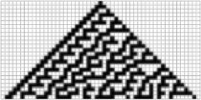
Figure 2: Rule 30 in motion: Here we can see several steps of the CA Rule 30 as presented in Figure 1. This is a one-dimensional lattice, with the downward vertical dimension representing successive time steps.

An example of a CA rule is given in figure 1. In brief, a CA is a state lattice with an update rule that updates the value of each lattice cell at each time step. The rule is local, in that the updated state for an individual cell depends only on the current states of the cell itself and of its neighbour cells. The set of cells on which the updated value of cell $x$ depends is called the neighbourhood of $x$. The size and form of the neighbourhood may vary from CA to CA.

We can see the time evolution of the rule in Figure 2.

In order to quantize the CA model, it is desirable to first make the model reversible. On the other hand, reversible computing predates quantum computing by several decades. One way to ensure that a CA is reversible is to use a Margolus partitioning scheme, in which the lattice is divided into tiles. A reversible operation is performed on each tile. On consecutive time-steps the tiling is staggered to allow the possibility of data propagation (see Figure 3).

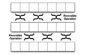
Figure 3: Margolus Partitioning CA Scheme

2.1 Quantum Cellular Automata

We wish to to formulate a model for quantum cellular automata. Several properties are desirable:

• The model should be a generalization of the classical CA and subsume the latter as a special case.

• The model should allow for quantum computation; it should be equivalent to the quantum circuit model.

• The model should ideally be reversible.

• The model should be a natural abstraction for quantum computation on particular realistic devices.

With this in mind, we first present a generic, basic model which will be our starting point for all our QCA studies.

2.1.1 The Basic Model

In our quantum cellular automaton model, we consider qubits arranged in an integer lattice of dimension $d$, $\mathbb{Z}^{d}$.

Instead of trying to define an state on an infinite lattice, we define a state $\rho$ as a family of states on finite subsets of the lattice. For each finite $A\subseteq\mathbb{Z}^{d}$, we take $\rho_{A}$ to be a state in the Hilbert space $\mathcal{H}^{\otimes A}$ over the subset $A$. The family of states $\rho=\{\rho_{A}\}_{A\subseteq\mathbb{Z}^{d},A\textrm{ finite}}$ must also satisfy a consistency condition. For every finite subset $A\subseteq\mathbb{Z}^{d}$, given $B\subseteq A$, we must have

$$\rho_{B}=\mathrm{tr}_{A\setminus B}(\rho_{A}).$$

In other words, partial traces must be consistent.

For a QCA, we must also have a global evolution operator. However, for any particular qubit in the lattice, interactions in one time-step must be localized to within a given neighbourhood of the qubit. To this end, we will first define a neighbourhood scheme as a finite set $N$ of elements of $\mathbb{Z}^{d}$ which includes the zero vector $0$, and then for each given lattice position $x$, we define the the neighbourhood of $x$ to be $\mathcal{N}(x)=x+N$. For a finite subset $A\subseteq\mathcal{Z}^{d}$, we will define $\mathcal{N}(A)$ to be the union of the neighbourhoods of the elements of $A$. Naturally, neighbourhood sets are translation independent, that is, given a lattice translation $\tau$, we have $\mathcal{N}(\tau(x))=\tau(\mathcal{N}(x))$.

Now, given a finite subset $A\subseteq\mathbb{Z}^{d}$, the result of a global evolution operator can be determined from its action on the subset $\mathcal{N}(A)$. Accordingly, we define our global evolution operator $U$ as a family of unitary operators $U_{\mathcal{N}(A)}$ acting on neighbourhoods for every finite subset $A\subseteq\mathbb{Z}^{d}$. The action of $U$ on a given state $\rho$ is given by

$$(U\rho)_{A}=\mathrm{tr}_{\mathcal{N}(A)\setminus A}\left(U_{\mathcal{N}(A)}\rho_{\mathcal{N}(A)}U^{\dagger}_{\mathcal{N}(A)}\right).$$

Of course, we also require $U$ to satisfy translation independence, so that for any subset $A\subseteq\mathbb{Z}^{d}$ and lattice translation $\tau$, we have $U_{\mathcal{N}(\tau(A))}=\tau(U_{\mathcal{N}(A)})$.

2.1.2 Deriving Global and Local Operators

We consider the operator $U$, consisting of a unitary operator $U_{\mathcal{N}(A)}$ for each finite subset $A\subseteq\mathbb{Z}^{d}$, as the global evolution operator for a given cellular automaton. From this, it would be desirable to find a local operator, which could reciprocally be used to derive the global operator.

The unitary operator $U_{\mathcal{N}(x)}$, corresponding to the subset $\{x\}$ consisting of a single element, makes a natural choice for a local operator. However, deriving the global operator from this requires some work, as we require a family of unitary operators which satisfy the consistency condition for each finite subset of $\mathbb{Z}^{d}$.

To this end, for the qubit at lattice position $x$, we define $S_{x}^{0}$ to be the set of pure states $|\psi\rangle$ over the lattice subset $\mathcal{N}(x)$ which satisfy

$$\mathrm{tr}_{\mathcal{N}(x)\setminus\{x\}}\left(U_{\mathcal{N}(x)}|\psi\rangle\!\langle\psi|U_{\mathcal{N}(x)}^{\dagger}\right)=|0\rangle\!\langle 0|,$$

and similarly, we define $S_{x}^{1}$ to be the set of pure states which map to $|1\rangle\!\langle 1|$. In general, the set $S_{x}^{j}$ is an affine space for which a basis may be computed for any given $U_{\mathcal{N}(x)}$. We may also consider the affine spaces $S_{x}^{j}$ as sets of states over a larger finite subset of $\mathbb{Z}^{d}$ containing $x$.

Now, given a finite subset $A\subseteq\mathbb{Z}^{d}$, with $A=\{x_{1},\ldots,x_{n}\}$, the set of lattice states which maps to a particular state $|j\rangle=|j_{1},\ldots,j_{n}\rangle$ on the lattice subset $A$ will be

$$S_{A}^{j}=\bigcap_{k=1}^{n}S_{x_{k}}^{j_{k}},$$

where the sets $S_{x_{k}}^{j_{k}}$ are considered as sets of states over the lattice subset $\mathcal{N}(A)$.

By selecting a basis for the set of states over the lattice points in $\mathcal{N}(A)\setminus A$ for each $j$, it is possible to find a unitary operator $U_{\mathcal{N}(A)}$ that makes the appropriate map, so any vector in $S_{A}^{j}$ is properly mapped to $|j\rangle$. In addition, note that in order for $U_{A}$ to satisfy the consistency condition, vectors outside $S_{A}^{j}$ must not be mapped to $|j\rangle$. Since every vector in $S_{A}^{j}$ must be mapped to something, it must be $|j\rangle$. Thus every operator $U$ that satisfies the consistency condition can be constructed in this way. Also, note that while we have many choices for any particular operator $U_{A}$, every choice yields the same result after the partial trace. Next, we will show these operators are always consistent.

In order to be a proper global transition operator, $U$ must preserve the consistency condition. That is, given a state $\rho$, and given that $\sigma=U\rho$, we must have

$$\sigma_{A}=\mathrm{tr}_{B\setminus A}(\sigma_{B})$$

for every finite subset $B\subseteq\mathbb{Z}^{d}$ and for any $A\subseteq B$. In other words, we must have

$$\mathrm{tr}_{\mathcal{N}(A)\setminus A}\left(U_{\mathcal{N}(A)}\rho_{\mathcal{N}(A)}U^{\dagger}_{\mathcal{N}(A)}\right)=\\ \mathrm{tr}_{B\setminus A}\mathrm{tr}_{\mathcal{N}(B)\setminus B}\left(U_{\mathcal{N}(B)}\rho_{\mathcal{N}(B)}U^{\dagger}_{\mathcal{N}(B)}\right),$$

given that $\mathrm{tr}_{\mathcal{N}(B)\setminus\mathcal{N}(A)}\rho_{\mathcal{N}(B)}=\rho_{\mathcal{N}(A)}$

Since both $U_{\mathcal{N}(A)}$, $U_{\mathcal{N}(B)}$ and the partial trace are linear functions, it suffices to show that this relation holds for operators of the form $\rho_{\mathcal{N}(B)}=|\psi\rangle\!\langle\phi|$, where $|\psi\rangle\in S_{B}^{j}$ and $|\phi\rangle\in S_{B}^{k}$ for computational basis states $|j\rangle$ and $|k\rangle$ over $B$. But by definition, we also have $|\psi\rangle\in S_{A}^{j}$ and $|\phi\rangle\in S_{A}^{k}$, and so both sides of the above identity equal $\mathrm{tr}_{B\setminus A}|j\rangle\!\langle k|.$

Therefore, an operator $U$ is valid if and only if it is the same as the one constructed by the local operator, up to unitary operators acting on $\mathcal{N}(A)\setminus A$.

3 QCA Models

Now that we have shown our general QCA model, we can introduce particular varieties of QCA types as instances of our model. The first one we introduce is the Margolus QCA, or MQCA.

3.1 Margolus QCA

The MQCA is similar to its classical counterpart, in which we define a tiling of the lattice, and apply the same unitary operation to each tile. The tiling is then changed in such a way that each tile of one tiling overlaps with at least two tiles of the original one. The two tilings need not have equally shaped tiles, but must have the same period with respect to the lattice (see Figure 4).

Figure 4: Margolus QCA: Similar to the classical reversible CA, the lattice is partitioned using two different tiling sets. Each tile is then acted on with a unitary operator.

Formally, we state:

Definition 1.

A Margolus partitioning is a pair of array partitions $k$ and $r$, dividing the lattice into collections of identical, finite, disjoint, and uniformly arranged blocks, such that each block of one partition overlaps with at least two from the other. A Margolus Quantum Cellular Automata (MQCA) is defined by lattice $S$ a Margolus partitioning of $S$ and a pair $U,V$ of unitary transformations, each one acting on the blocks of one of the partitionings.

It is easy to see that the MQCA follows the consistency conditions outlined above. An interesting example of an MQCA is the multi-particle quantum walk.

Example 1.

Let $S$ be $\mathbb{C}^{\mathbb{Z}}$, the integer line. The partitionings $p$ and $s$ both divide the lattice into blocks of two qubits, each block overlapping one qubit from one block in the other partitioning, as in Figure 4. Let

$$u=v=\left(\begin{array}[]{cccc}1&0&0&0\\ 0&\frac{1+i}{2}&\frac{-1+i}{2}&0\\ 0&\frac{-1+i}{2}&\frac{1+i}{2}&0\\ 0&0&0&1\\ \end{array}\right).$$

For this example, in the computational basis, we understand a $1$ to represent the presence of a particle, and zero to represent the abscence. The overall effect is that any particles in the lattice slowly get diffused over time. There is no interaction among particles.

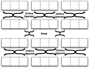
Figure 5: Partitioned QCA: In a PQCA each cell is partitioned into 3 ‘subcells’: left, centre, and right.. A unitary operator is applied to each cell at odd time steps, and at even time steps the cells exchange subcells, it’s right subcell is exchanged with the left subcell of the right neighbour, and the left subcell is exchanged with the right subcell of the left neighbour.

Both van Dam [1] and Watrous [2] consider partitioned QCA or PQCA. A PQCA is shown in detail if figure 5. This scheme is simply a particular kind of Margolus partitioning; one of the Margolus partitioning operators is simply a swap.

It should be pointed out, though, that the van Dam and Watrous model differs greatly from the one presented here. In their model, the quantum state of QCA is in a superposition of classical configurations of the lattice. This leads to a very different definition of the evolution operator as well, which runs into problems as outlined in [3]. Type-II quantum [16, 17], computers can be regarded as particular instances of the PQCA scheme, except that the exchange procedure is done non-coherently.

The example we chose also has a historical significance. Quantum walks on a lattice have been extensively studied before (see for example [4] for an overview)), and in particular a QCA quantum walk has been analyzed in [5]. It is of note that one can take the continuous limit of the walk we outlined above, i.e. the limit when the space between lattice cells and the duration of the time step both go to zero. Doing so gives the Schrödinger equation for a particle in free motion [5]. This works for lattices of any dimension. By taking the limit in a slightly different way one can obtain the Dirac equation; although this works only for one dimensional systems at the moment [6].

Also, in [3] Schumacher and Werner show that MQCA are universal QCA, in the sense that all QCA (as defined in their general scheme) can be reduced to MQCA.

More recently, Raussendorf shows how to build a universal quantum computer using a Margolus style quantum cellular automata [7]. For these reasons, implementing a MQCA on a physical device would be of great usefulness. We explore this in our next section.

3.2 Colored QCA

In 1993 S. Lloyd introduced an example of a (time-inhomogenous) CQCAs, which we will call Spin-chain QCA. He introduced this model as a proposal for a feasible quantum computer. Consider a one-dimensional chain of spin $1/2$ systems, such as a polymer, with three different species, i.e $ABCABC\ldots$

Suppose that the nearest-neighbour interactions are given by (arbitrary) Hamitlonians $H_{AB}$, $H_{BC}$, $H_{CA}$. In the computational basis, the diagonal terms of this Hamiltonian shift the energy levels of each cell as a function of the energy levels of its neighbours [8].

The resonant frequency $\omega_{A}$ can then take the value $\omega^{A}_{00}$, $\omega^{A}_{01}$, $\omega^{A}_{10}$, or $\omega^{A}_{11}$, depending on whether its $C$ and $B$ neighbours are in the states $0$ and $0$, $0$ and $1$, $1$ and $0$, or $1$ and $1$.

Hence, chain link $A$ with neighbours $C$ and $B$ has resonant frequency $\omega_{A}$ with distinguishable diagonal terms $\omega^{A}_{00}$, $\omega^{A}_{01}$, $\omega^{A}_{10}$, and $\omega^{A}_{11}$. If these are all different, then transitions on species $A$ spins can be done selectively depending on the value $k$. For instance, by applying a $\pi$ pulse with frequency $\omega^{A}_{00}$ all species $A$ lattice points whose both neighbours are in the state $0$ will be flipped.

It is also possible to apply, using the same techniques, any arbitrary single-qubit gate to all spins of the same species and to apply any two qubit gate on all pairs $A,B$ or $C,A$ or $B,C$.

We introduce a new general QCA model, which we call Coloured QCA (CQCA). This model is a generalization and abstraction of Lloyd’s scheme.

Figure 6: Colored QCA This is a representation of a one-dimensional CQCA, with time going downward. The two shades of gray differentiate between the two species in this CQCA. The brackets represent the controlled unitaries: at each step either the light or dark grey sites are acted on with unitary operators that depend on their left and right neighbour values.

In a CQCA, each lattice point is assigned a colour in a checkerboard fashion. At each time step only points of a certain colour are updated with a unitary dependant on their neighbour’s values. Neighbours of the same colour are not distinguishable.

A graphical representation is shown in Figure 6, and a formal definition is given below.

Definition 2.

A correct $k$-colouring for a lattice is a periodic mapping $C$ from lattice points to $\{0,\ldots,k-1\}$, such that no two neighbours have the same colour. Fix a single qubit observable $\sigma$. For each lattice cell $t$ its $l$-field is the value $\sum_{r\in N(t),C(r)=l}\langle\psi|\sigma^{(r)}|\psi\rangle$. A field-controlled unitary $u$ is such that it is only applied to a lattice point if its l-field, for $l\in\{0,\ldots,k-1\}$ has a particular set of values.

A Coloured QCA or CQCA is defined by a neighbouring $N$, colouring $C$, and a field-controlled unitary $u_{l}$ for each colour $l\in\{0,\ldots,k-1\}$.

Again, it is not hard to see that CQCA adhere to the consistency constraints outlined in our generic model.

Several proposal for implementation of quantum computers can be seen as instances of the CQCA model. Obviously, Lloyd’s pulse-drvien quantum computers are one example. Benjamin’s proposal [9] is an example of 2-CQCA scheme that achieves universality. K. G. H. Vollbrecht and J. I. Cirac [10] present a 1-CQCA (each lattice site being a qudit with $d=4$), that also achieves universality.

Example 2.

An example of a proper CQCA is the 1-D quantum walk CQCA. As in Example 1 above, let $S$ be $\mathbb{C}^{\mathbb{Z}}$, the integer line. The colouring scheme uses four colours $\{c_{i}\}_{0\leq i\leq 3}$ such that position $x_{i}$ on the lattice has colour $i\mod 4$.

The evolution operator is as follows. First, $c_{1}$ is given a $\pi$ z-rotation conditioned on $c_{0}$ being in $|1\rangle$. Then $c_{0}$ is given a $\pi/2$ z-rotation conditioned on $c_{1}$ being in $|1\rangle$. Then we repeat the $\pi$ z-rotation on $c_{1}$ conditioned on $c_{0}$ being in $|1\rangle$. We can see that this procedure is equivalent to doing a square-root-of-swap on all pairs $c_{0}$-$c_{1}$. We do the same procedure on colours $c_{2}$-$c_{3}$, and then on both pairs $c_{1}$-$c_{2}$ and $c_{3}$-$c_{0}$.

The above construction gives the exact dynamics as the MQCA of Example 1 above, namely, a quantum walk on the line.

From the example above, one might deduce that any dynamic given in the MQCA model can also be constructed using CQCA. This is in fact true, and is proven below.

Theorem 1.

For every MQCA there exists a CQCA, and for every CQCA there exists and MQCA that has the exact same dynamics.

Proof.

For this proof we rely on the fact that arbitrary single qubit operations, coupled with c-NOT gates on adjacent qubits (for a connected topology) is universal for quantum computation.

We proceed constructively. Given an MQCA $M$, with partitions $s$, $t$, we can build a CQCA $C$ that has the exact same dynamics as follows.

The lattice of $M$ will be the same lattice for $S$. Without loss of generality suppose that the partition $s$ has more lattice sites per block than $t$. Let $k$ be the number of sites in each block of $s$. We construct our $CQCA$ with $2s$ colours. The colour mapping is such that each partition block of $M$ is represented by $s$ distinct colours in $C$ (each block having the exact same colours as each other block in the partition), and two neighbouring block has two similar colours.

Now, we can simulate any arbitrary unitary acting on a block of $M$ using only colour-controlled operations in $C$: since each spin in the block has a distinct colour, they are all individually addressable. Moreover, we can apply c-NOT gates between any two neighbouring spins. Operations on $C$ will be repeated periodically over the lattice, due to the repeating colour scheme, and hence it is important that block boundaries coincide with colour periodicity.

Also we use $2s$ colours instead $s$, so it is necessary to repeat the operations on $C$ for alternating blocks of $M$. This is necessary to ensure that we can isolate each block in order to perform arbitrary operations on it.

∎

The importance of the above theorem, beyond mathematical curiousity, is that it allows us a simple way to implement MQCA algorithms on physical devices.

3.3 Continuous-Time QCA

Another model we present is the Continuous Time QCA (CTQCA).

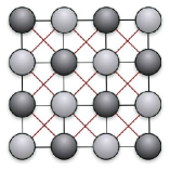
Figure 7: Continuous Time QCA: We have a crystal with two types of nuclei $A$ and $B$, one represented as light gray spheres, the other dark gray. The lines connecting the spheres represent the nearest neighbour couplings, with different colour lines representing different coupling Hamiltonians. Notice that the coupling Hamiltonian depends only on the colour of the coupled spins.

A CTQCA is similar to a CQCA in that all lattice points are coloured. However, instead of unitary operators applied in discrete timesteps, the system evolves continuously according to a Hamiltonian described only by nearest neighbour couplings.

Definition 3.

Let $C$ be any colouring, that is any periodic mapping from lattice points to $\{0,\ldots,k-1\}$, but not necessarily ‘correct’ in the sense of Definition 2 above.

Every pair of neighbouring lattice points $i,j$ has a coupling Hamiltonian $H_{i,j}(t)$ that depends only on the colour of the two points. For a given region of the lattice, the Hamiltonian of that region is simply

$$H(t)\sum_{i<j}H_{i,j}(t).$$

The evolution of the CTQCA over a given time period $t$ is given by

$$U[t]=\int e^{iH(t)}dt.$$

A good example of a CTQCA is the diffusion automata as defined below.

Example 3.

Again, as in example 1 above Let $S$ be $\mathbb{C}^{\mathbb{Z}}$, the integer line. The colouring scheme requires only one colour, and each spin has only two neighbours, one directly to its left, and to its right. The coupling Hamiltonian is

$$H=\sum_{i}\sigma_{+}^{(i)}\sigma_{+}^{(i+1)}+\sigma_{-}^{(i)}\sigma_{-}^{(i+1)}$$

In solid-state NMR this is called the flip-flop coupling, since it has the effect of flipping two contiguous spins from $|01\rangle$ to $|10\rangle$.

The evolution of this CTQCA is similar to the quantum walks of Examples 1 and 2 above. Again this is not coincidental.

An important result is that CTQCA is, again, an equivalent computational model to the other QCA models presented above.

Theorem 2.

Given, a CQCA there is a CTQCA that has the same dynamics.

Proof.

This construction is very simple. Given a a CQCA $C$ we can construct a CTQCA $T$ with the same lattice and same colour-scheme. We give a time-dependant Hamiltonian $H$ that changes at discrete time-steps of duration $t$ so that $U=e^{itH}$ where $U$ is the unitary of the CQCA at the given timestep.

∎

The converse is slightly more complicated, and can only be done in an approximate sense,

Theorem 3.

Let $\Delta T$ be the time it takes to do one time step. Then, a CQCA $C$ can approximate a CTQCA $T$ when $\Delta T\rightarrow 0$.

Proof.

Continuous time QCA, as opposed to CQCA do not have the restriction that neighbours cannot be of the same colour. Assuming that the colouring is correct for the given CTQCA $T$, then we proceed as follows.

Let $C$ have the same colour scheme as $T$.

For any pair of colours $t_{i}$ and $t_{j}$ let $H_{i,j}$ be the coupling Hamiltonian for neighbours of that colour. Let $U_{i,j}[t]=e^{-itH}$. Now, $U_{i,j}[t]$ acts only on two spins, and hence can be described as a series of controlled operations, $U_{i,j}^{(i,1)}[t]$, $U_{i,j}^{(j,1)}[t]$, $U_{i,j}^{(i,2)}[t]$, $U_{i,j}^{(i,1)}[t]\ldots$ where $U_{i,j}^{(i,s)}[t]$ is an operation on the spin of colour $i$ controlled by the spin $j$, and so forth. These $U_{i,j}^{(r,s)}[t]$ become the controlled operators in our CQCA $C$. By letting $t\leftarrow 0$ the evolution of $C$ approximates the evolution of the CTQCA $T$.

If $T$ has neighbours of the same colour, we simply break any colour that has neighbouring spins into two or more colours, such that there are no longer neighbouring spins of the same colour. All the colours created this way will have the same coupling Hamiltonian to each other as the original colour had with itself. We can then apply the procedure outlined above.

∎

4 Conclusions

In closing we wish to give a summary of the contributions of this paper. First we gave a simple scheme for QCA that is general enough to encompass previous models of QCA, as well as other phenomenae studied under different names.

We gave several specific models, under this scheme, and we showed the relationship among this models. We posit that our model is not overly general, that is it describes all well formed QCA style phenomana and nothing else. This latter statement, though, is posited without proof.

5 Acknowledgements

Research for this paper was supported in part by ARDA, ORDCF, CFI, MITACS, and CIAR.

References

- [1] W. van Dam, Quantum cellular automata, citeseer.ist.psu.edu/vandam96quantum.html.
- [2] J. Watrous, On one-dimensional quantum cellular automata, in 36th Annual Symposium on Foundations of Computer Science (Milwaukee, WI, 1995), pp. 528–537, IEEE Comput. Soc. Press, Los Alamitos, CA, 1995.
- [3] R. W. B. Schumacher, (2004), quant-ph/0405174.
- [4] A. Ambainis, (2004), quant-ph/0403120.
- [5] B. M. Boghosian and W. Taylor IV, (2003), quant-ph/0308113.
- [6] D. A. Meyer, J. Statist. Phys. 85, 551 (1996).
- [7] R. Raussendorf, (2004), quant-ph/0412048.
- [8] S. Lloyd, Science 261, 1569 (1993).
- [9] S. C. Benjamin, Phys. Lett. B393, 132 (1999), quant-ph/9909007.
- [10] K. G. H. Vollbrecht and J. I. Cirac, (2005), quant-ph/0502143.
- [11] C. Dürr and M. Santha, SIAM J. Comput. 31, 1076 (2002).
- [12] A. Bririd and S. C. Benjamin, (2003), quant-ph/0308113.
- [13] R. Raussendorf, (2005), quant-ph/0505122.
- [14] D. Gottesman, Beyond the DiVincenzo criteria: Requirements and desiderata for fault-tolerance, in Joint IPAM/MSRI Workshop on Quantum Computing, 2002.
- [15] T. Toffoli and N. Margolus, Cellular Automata Machines (MIT Press, 1987).
- [16] P. J. Love and B. M. Boghosian, (2005), quant-ph/0506244.
- [17] P. J. Love and B. M. Boghosian, (2005), quant-ph/0507022.
- [18] D. A. Meyer, (1997), quant-ph/9703027.