Decoherence induced by a fluctuating Aharonov-Casher phase

Abstract

Dipoles interference is studied when atomic systems are coupled to classical electromagnetic fields. The interaction between the dipoles and the classical fields induces a time-varying Aharonov-Casher phase. Averaging over the phase generates a suppression of fringe visibility in the interference pattern. We show that, for suitable experimental conditions, the loss of contrast for dipoles can be observable and almost as large as the corresponding one for coherent electrons. We analyze different trajectories in order to show the dependence of the decoherence factor with the velocity of the particles.

I Introduction

Interference effects are the most distinguished characteristic of quantum mechanics. The double-slit experiment is often used as the starting point to quantum description of Nature. There, when the path of the interfering particles is measured, the interference pattern disappears and the classical picture is recovered. The interaction between the quantum system with its environment (measuring apparatus) is responsible for the process of decoherence, which is one of the main ingredients in order to reach the quantum-to-classical transition.

The Aharonov-Bohm (AB) aharonov interference experiment can be a realistic probe for the predictions of decoherence. This experiment starts by the preparation of two electron wave packets $\varphi_{1}(\vec{x})$ and $\varphi_{2}(\vec{x})$ in a coherent superposition, assuming each of the charged particles follows a well defined classical path ($C_{1}$ and $C_{2}$, respectively). The complete wave function involves the presence of the environment, given an state

$$\psi(t=0)=\left[\varphi_{1}(\vec{x})+\varphi_{2}(\vec{x})\right]\otimes\chi_{0}(\vec{y}),$$ (1)

where $\chi_{0}(\vec{y})$ represents the initial quantum state of the environment (whose set of coordinates is denoted by $\vec{y}$). As time follows, the electron’s coherent state entangles with the environment, and the total wave function can be described as

$$\psi(t)=\varphi_{1}(\vec{x},t)\otimes\chi_{1}(\vec{y},t)+\varphi_{2}(\vec{x},t)\otimes\chi_{2}(\vec{y},t).$$ (2)

Therefore, the two delocalized electron states $\varphi_{1}$ and $\varphi_{2}$ become correlated with two different states of the environment. The probability of finding a particle at a given position at time $t$ (for example when interference pattern is examined) is,

$$\mbox{Prob}(\vec{x},t)=|\varphi_{1}(\vec{x},t)|^{2}+|\varphi_{2}(\vec{x},t)|^{2}+2{\rm Re}\left(\varphi_{1}(\vec{x},t)\varphi^{*}_{2}(\vec{x},t)\int d^{3}y~{}\chi_{1}^{*}(\vec{y},t)\chi_{2}(\vec{y},t)\right).$$ (3)

The overlap factor $F=\int d^{3}y~{}\chi_{1}^{*}(\vec{y},t)\chi_{2}(\vec{y},t)$ is responsible for two separate effects. Its phase generates a shift of the interference fringes, and its absolute value is responsible for the decay in the interference fringe contrast. Of course, in absence of environment the overlap factor is not present in the interference term. When the two environmental states do not overlap at all, the final state of the bath identifies the path the electron followed. There is no uncertainty respect to the path. Decoherence appears as soon as the two interfering partial waves shift the environment into states orthogonal to each other. Last statement suggests that the environment saves (in some way) the information about the path the electron takes.

The loss of quantum coherence can alternatively be explained by the effect of the environment over the partial waves, rather than how the waves affect the environment. As has been noted, when a static potential $V(x)$ is exerted on one of the partial waves, this wave acquires a phase,

$$\phi=-\int V[x(t)]dt,$$ (4)

and therefore, the interference term appears multiplied by a factor $e^{i\phi}$. This is a possible agent of decoherence. The effect can be directly related to the statistical character of $\phi$, in particular in situations where the potential is not static. Even more, any source of stochastic noise would create a decaying coefficient. For a general case, $\phi$ is not totally defined, i.e. it is described by means of a distribution function $P(\phi)$. From this statistical point of view, the phase can be written as

$$\langle e^{i\phi}\rangle=\int e^{i\phi}P(\phi)d\phi.$$ (5)

In this way, the uncertainty in the phase produces a decaying term that tends to eliminate the interference pattern. This dephasing is due to the presence of a noisy environment coupled to the system and can be also represented by the Feynmann-Vernon influence functional formalism. It is easy to prove that Eq.(5) is the influence functional generated after integrating out the environmental degrees of freedom of an open quantum system. Therefore, in Ref. stern was shown the formal equivalence between the two ways of studying dephasing

$$\langle e^{i\phi}\rangle=F=\int d^{3}y~{}\chi_{1}^{*}(\vec{y},t)\chi_{2}(\vec{y},t).$$ (6)

The overlap factor $F$ encodes the information about the statistical nature of noise. Therefore, noise (classical or quantum) makes $F$ less than one, and the idea is to quantify how it slightly destroys particle interference pattern.

In many cases, the interaction with the environment cannot be switched off. Thus, for charged particles or neutral atoms with dipole moment, the interaction with the electromagnetic field is crucial. This interaction induces a reduction of fringe visibility. For example, vacuum fluctuations of electromagnetic fields have been considered as a decoherent agent villa . Double-slit-like experiments were studied in the presence of conductors, which change the structure of vacuum and modify predictions about decoherence effects. The changes on the fringe visibility induced by the position and relative orientation of the conductors are rather small.

Electron interference in mesoscopic devices irradiated by external nonclassical microwaves was considered in Ref. vourdasPRA02 . The effect of quantum noise on electron interference for several types of microwaves has been analyzed, and it was shown that entangled electromagnetic fields interacting with electrons produce entangled photons vourdasPRA04 . Despite the quantum nature of noise (vacuum fluctuations for example), classical noise is also present when considering time dependent fields, or some random variables that parametrize the environment. The destruction of electron interference by external classical and quantum noise has been studied in Ref. vourdasPRA01 .

In Ref. ford , the overlap factor $F$ was evaluated from a different point of view. They studied the effect of time-varying electromagnetic fields on electron coherence, including the statistical origin of the AB phase $\phi$. However, they didn’t consider $\phi$ neither as coming from quantum fluctuations nor a time dependent field. They included a random variable $t_{0}$, which was defined as the electron emission time. This variable produces a fluctuating phase $\phi$, and an average over it is needed in order to obtain the result of the double-slit interference experiment. In this simple version of decoherence, the role of a quantum environment is replaced by a time-dependent external field which gives a time-varying AB phase. The authors have considered the case of a linearly polarized, monochromatic electromagnetic wave, propagating in a direction orthogonal to the plane containing two electron beams. The effect on the fringes seems to be sufficiently large to be observable.

In the present article we follow last idea. We evaluate the overlap factor $F$ for coherent neutral particles with permanent (electric and magnetic) dipoles that are affected by time-varying external fields. We consider two different cases with possible experimental interest: firstly, the case of dipoles interacting with a linearly polarized electromagnetic plane wave. This will generalize results of Ref. ford to the case of Aharonov-Casher (AC) casher case in atomic systems sangster , where coherent dipoles follow a closed path around an external field. Secondly, the case of dipoles travelling through a waveguide with rectangular section. As we will discuss, not all these effects foresee an observable displacement on the interference pattern related to the phase shift of the wave function of the system. Dependence on the velocity of the interfering particle is crucial. We will show different configurations where the decoherence factor depends on the particle’s speed in a different way.

In principle, for neutral particles with the same mass and velocity than the charged ones, one should expect the loss of contrast for dipoles to be smaller than the analogous one in experiments performed using charged particles. Although this is basically true, the interaction between electromagnetic fields and dipoles is also weaker, allowing to increase the intensity of external classical fields in the same amount than the dipole effect is smaller, still neglecting the dipole scattering in the external field. Therefore, for sufficiently strong external fields, the effect on fringe visibility for dipoles will be of comparable magnitude with respect to the case of charged particles. In order to prove this, we will evaluate the scattering cross section for dipoles in interaction with both a plane wave and the fields inside a waveguide.

The paper is organized as follows. In Section II we present the evaluation of the phase shift and the decoherence factor for coherent dipoles (electric and magnetic) in the presence of a time varying electromagnetic plane wave. Symmetric and non-symmetric trajectories are considered in order to analize the dependence on the velocity of the interfering particles. We also include in this section some new results for charged particles. Section III shows the results when the coherent trajectories are inside a waveguide. In Section IV we estimate the decoherence factor for realistic values of the different parameters, and compare the loss of contrast for charged particles and dipoles. Section V contains our final remarks. We also include an Appendix where we compute the Thomson cross section for dipoles.

II Coherent dipoles and a plane wave

The AB phase aharonov , known to arise when two coherent electrons traverse two different paths $C_{1}$ and $C_{2}$ in the presence of an electromagnetic field, is ($c=\hbar=1$)

$$\phi=-e\oint_{\delta\Omega}dx_{\nu}A^{\nu}(x),$$ (7)

where $\delta\Omega=C_{1}-C_{2}$ is a closed spacetime path. If the electromagnetic field’s fluctuations happen in a time scale shorter than the total time of the experiment, this shift of phase results in a loss of contrast in the interference fringes. Then, the overlap factor (or decoherence factor) is given by Eq.(6) stern ; ford . In that expression, angular brackets denote either an ensemble of quantum noise or a time average over a random variable.

The classical and quantum interaction of a dipole with an arbitrary electromagnetic field has been described in detail in Ref. anandan , where a unified and fully relativistic treatment of this interaction has been presented. The Lorentz-invariant, classical interaction Lagrangian is $\frac{1}{2}P_{\mu\nu}F^{\mu\nu}$ where $P_{\mu\nu}$ is the antisymmetric dipole tensor villa ; anandan . In the rest frame of the particle, the electric ($\mathbf{d}$) and magnetic ($\mathbf{m}$) dipole moments can be obtained from $P_{0i}=d_{i}$ and $P_{ij}=\epsilon_{ijk}m_{k}$ respectively.

In the quantum case, the phase shift that two neutral particles with electric and magnetic dipole moments experience due to a classical time dependent electromagnetic field is known as the Aharonov-Casher phase casher and is defined by

$$\phi=-\oint_{\delta\Omega}a_{\nu}(x)dx^{\nu},$$ (8)

where $a_{\nu}(x)=(-\mathbf{m}\cdot\mathbf{B}-\mathbf{d}\cdot\mathbf{E},\mathbf{d}\times\mathbf{B}-\mathbf{m}\times\mathbf{E})$ plays the role of $A_{\nu}$ in the AB case, $\delta\Omega=C_{1}-C_{2}$, and $C_{1}$ and $C_{2}$ are the two paths followed by the particles that interfere.

In order to evaluate the integral in Eq.(8), we consider the case of a linearly polarized monochromatic wave of frequency $\omega$ propagating in the $\hat{y}$ direction, with an electric and magnetic field in the $\hat{z}$ and $\hat{x}$ direction respectively. We will also assume that the particles’ path is confined to the $\mathit{{\hat{x}}-{\hat{z}}}$ plane (see Fig. 1). We can write the plane wave as $\mathbf{E}(x)=E_{0}\sin(wt-ky)~{}\hat{z}$, $\mathbf{B}(x)=E_{0}\sin(wt-ky)~{}\hat{x}$ and compute $a_{\nu}$, which is given by

$$a_{\nu}(x) = (-d_{z}E_{z}-m_{x}B_{x},m_{y}E_{z},d_{z}B_{x}-m_{x}E_{z},-d_{y}B_{x})$$ (9)

$$= E_{0}(-d_{z}-m_{x},m_{y},d_{z}-m_{x},-d_{y})\sin(\omega t-ky)$$

$$\equiv {\tilde{a}}_{\nu}\sin(\omega t-ky).$$

Following Ref. ford , we will assume that the phase $\phi$ depends on a random variable $\xi=\omega t_{0}$ given by the emission time of the dipoles. It is the time $t_{0}$ at which the center of a localized wave packet is emitted. When the measuring time takes longer than the flight time, we will observe a result which is the temporal average over $t_{0}$. Thus, $t_{0}$ is a random variable by which $\phi$ has to be averaged. We can write the AC phase $\phi$ as

$$\phi(t_{0})=-\oint_{\delta\Omega}{\tilde{a}}_{\nu}\sin(\omega t-ky+\omega t_{0})~{}dx^{\nu},$$ (10)

before taking the time average, we rewrite the phase as

$$\phi(t_{0})=A\cos(\omega t_{0})+B\sin(\omega t_{0}),$$ (11)

where

$$A = -\oint_{\delta\Omega}{\tilde{a}}_{\nu}(x)\sin(\omega t-ky)~{}dx^{\nu},$$

$$B = -\oint_{\delta\Omega}{\tilde{a}}_{\nu}\cos(\omega t-ky)~{}dx^{\nu}.$$ (12)

The average over the random phase (generating a classical noise) produces a decoherence factor

$$F=\langle e^{i\phi}\rangle=\lim_{T\rightarrow\infty}\frac{1}{2T}\int_{-T}^{T}dt_{0}\exp\left\{i\left[A\cos(\omega t_{0})+B\sin(\omega t_{0})\right]\right\}=J_{0}(|C|),$$ (13)

where $J_{0}$ is the Bessel function. The modulus of complex number $C=A+iB$ measures degree of decoherence. The overlap factor $F$ decreases from one to zero as $|C|$ varies between zero and the first zero of $J_{0}$. For larger values of $|C|$, the overlap factor oscillates with decreasing amplitude. For a Gaussian $P(\phi)$ distribution with $\langle\phi^{2}\rangle\ll 1$, we have, in the limit $|C|\ll 1$, $\langle e^{i\phi}\rangle\approx 1-\langle\phi^{2}\rangle=1-|C|^{2}/2$.

A characteristic feature of the usual AB and AC effects is that the phase shift is independent of the velocity berry of the particle and there is no force on the particle APV . Moreover, the phase shift depends only on the topology of the closed spacetime path $\delta\Omega$. Of course, these properties are not longer valid when the external field is time dependent because the particle does suffer a net force applied on it. Thus, in order to analyze the dependence upon the trajectory, we will evaluate Eq.(8) for different paths and will find that the phase’s dependence on the velocity is strongly related to the trajectory the particles follow.

II.1 Symmetric trajectories

In this subsection, we will estimate the phase acquired by two neutral particles with electric and magnetic dipole moments when they follow symmetric trajectories as the ones depicted in Fig. 1.

To begin with, we will consider the same trajectory used by authors in ford to analyze the AB phase factor between charged particles. To perform integration in Eq.(12) along the trajectory of Fig.1(a), we must calculate

$$\phi=\oint_{\delta\Omega}a_{\nu}(x)dx^{\nu}=\sum_{i=1}^{6}\int_{0}^{1}a_{\nu}(\sigma_{i}^{\nu}(u))\cdot\frac{d\sigma_{i}^{\nu}}{du}du,$$ (14)

where $\sigma_{i}$, with $i=1...6$, parametrize the different segments of the trajectory. The path of particle 1 (${\cal C}_{1}$) is described by:

$$\sigma_{1}(u) = (-T/2-\theta+\theta u,-d-l+ul,0,u\alpha)$$

$$\sigma_{2}(u) = (-T/2+Tu,-d+2du,0,\alpha)$$

$$\sigma_{3}(u) = (T/2+u\theta,d+ul,0,\alpha-u\alpha),\quad\quad\mathrm{for}\quad 0\leq u\leq 1.$$ (15)

Meanwhile the path of particle 2 (${\cal C}_{2}$) is:

$$\sigma_{4}(u) = (-T/2-\theta+\theta u,-d-l+ul,0,-u\alpha)$$

$$\sigma_{5}(u) = (-T/2+Tu,-d+2du,0,-\alpha)$$

$$\sigma_{6}(u) = (T/2+u\theta,d+ul,0,-\alpha+u\alpha),\quad\mathrm{for}\quad 0\leq u\leq 1.$$ (16)

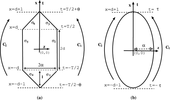
Figure 1: Paths ${\cal C}_{1}$ and ${\cal C}_{2}$ are shown for the (a) trajectory used in ford and (b) an elliptic one.

Performing the integrations in Eq.(14) and using the definition given in Eq.(12), we obtain $B_{d}=0$ and

$$|C_{d}|\equiv|A_{d}|=4E_{0}d_{y}\big{(}\frac{2\alpha}{\omega\theta}\big{)}\sin\big{(}\frac{\omega\theta}{2}\big{)}\sin\big{(}\frac{\omega(T+\theta)}{2}\big{)},$$ (17)

where $2\alpha$ is the maximum distance between the particles, $d_{y}$ is the electric dipole’s moment in the $\hat{y}$ direction and $T,\theta$ are characteristic times of the trajectory. The subindex $d$ indicates that these are the values of $A,B$ and $C$ for dipoles.

For non relativistic particles, we expect $\omega\theta,\,\,\omega T\gg 1$. Therefore, in order to have an estimation for $C_{d}$ we can replace the sine functions by a typical value $1/\sqrt{2}$. In order to make explicit the dependence on the velocity, note that $\theta=s/v$, where $s$ is the length of the first and third segments of the path defined by $s=\sqrt{\alpha^{2}+l^{2}}$. Using this, we rewrite Eq.(17) as

$$|C_{d}|\approx\frac{2}{\pi}E_{0}d_{y}\big{(}\frac{\alpha}{s}\big{)}\lambda v\approx\frac{2}{\pi}eE_{0}\big{(}\frac{\alpha}{s}\big{)}\lambda Lv.$$ (18)

Here $L$ is the characteristic length of an atom with electric dipole $d=eL$ ($L\approx 10^{-9}m$), and $\lambda$ is the wavelength of the plane wave. The analogous result for charged particles is given by $|C_{e}|\approx\frac{1}{\pi^{2}}eE_{0}\lambda^{2}(\frac{\alpha}{s})v$ ford . Assuming that the charged and neutral particles have the same speed and trajectory, for the same external field we obtain

$$|C_{d}|\approx|C_{e}|\bigg{(}\frac{L}{\lambda}\bigg{)}.$$ (19)

Even though Eq.(19) might be discouraging, the scattering cross section for neutral particles is much smaller than for charged particles (see Appendix). This makes it possible to increase the intensity of the external field and, consequently, the value of the decoherence factor at least some orders of magnitude.

If the neutral particles follow an elliptic path (Fig 1 (b)), the calculations proceed in a similar way. The trajectory is parametrized by

$$\sigma_{1}(u)=(\tau\sin(u),(d+l)\sin(u),0,~{}~{}\alpha\cos(u))\quad\quad\quad\mathrm{for}-\pi/2\leq u\leq\pi/2$$

$$\sigma_{2}(u)=(\tau\sin(u),(d+l)\sin(u),0,-\alpha\cos(u))\quad\quad\quad\mathrm{for}-\pi/2\leq u\leq\pi/2,$$ (20)

where $\tau$ is the time of flight of the dipoles and $(d+l)$ is the total length of the path. In this case, the quantity $|C^{d}_{\rm ellip}|$ is given by

$$|C^{d}_{\rm ellip}|=2\pi\alpha E_{0}d_{y}\mathrm{J}_{1}[\omega\tau],$$ (21)

with $\mathrm{J}_{1}$ the Bessel function of first order. Using the asymptotic expansion of this function for $\omega\tau\gg 1$ we find

$$|C^{d}_{\rm ellip}|\approx\frac{\sqrt{2}\pi\alpha E_{0}d_{y}}{(\omega\tau)^{1/2}}=\sqrt{\pi}\alpha eE_{0}L\left(\frac{v\lambda}{s^{\prime}}\right)^{1/2}$$ (22)

where $s^{\prime}$ is the length travelled by the neutral particles at a speed $v$ and in a time $\tau$. It is important to note that while $|C_{d}|$ in Eq.(18) depends linearly on the velocity, for the elliptic trajectory $|C^{d}_{\rm ellip}|$ scales as $\sqrt{v}$.

It is interesting to check whether the same difference in behaviours applies to the case of the AB phase for charged particles or not. If the charged particles travel across the paths shown in Fig.1(b), the quantity $|C^{e}_{\rm ellip}|$ can be computed from Eq.(7) and the parametrization Eq.(20). The result is

$$|C^{e}_{\rm ellip}|=2\pi\alpha eE_{0}\lambda\mathrm{J}_{1}[\omega\tau],$$ (23)

showing that the dependence on the velocity is similar for both neutral and charged particles.

Finally, it is worth noting that, as both trajectories in Figs.1(a) and (b) are symmetric respect to the $\hat{x}$ ($\hat{t}$) axis, only the term proportional to $A$ of Eq.(12) contributes to the AC phase, and, consequently, to the decoherence factor. This is due to the parity of the integrand with respect to $x$ and $t$.

II.2 Asymmetric trajectory

In this subsection we will consider the case of dipole wave packets travelling across the asymmetric trajectory depicted in Fig. 2. As we will see, in this case, not only do both terms in Eq.(12) contribute to the AC phase but also different components of the dipole moments. Consequently, speed dependence will be different from the case of symmetric trajectories.

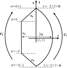
Figure 2: Paths ${\cal C}_{1}$ and ${\cal C}_{2}$ are shown for the asymmetric trajectory.

We write $C^{d}_{\rm asym}=A^{d}_{\rm asym}+iB^{d}_{\rm asym}$, where each of these coefficients is defined in Eq.(12). The parametrization of the asymmetric curve can be read from Eqs.(15) and (20). After performing the corresponding integrations, we obtain

$$A^{d}_{\rm asym} = \pi d_{y}E_{0}\alpha\mathrm{J}_{1}[\omega\tau]+\frac{4E_{0}d_{y}\alpha}{\omega\theta}\sin[\frac{\omega\theta}{2}]\sin[\frac{\omega}{2}(T+\theta)],$$

$$B^{d}_{\rm asym} = (d_{z}+m_{x})\frac{2E_{0}}{\omega}\left[\sin[\frac{\omega\theta}{2}]\cos[\frac{\omega}{2}(T+\theta)]+\sin[\frac{\omega T}{2}]\right]$$ (24)

$$+ \frac{2m_{y}E_{0}l}{\omega\theta}\sin[\frac{\omega\theta}{2}]\cos[\frac{\omega}{2}(T+\theta)]+\frac{4dE_{0}m_{y}}{\omega T}\sin[\frac{\omega T}{2}].$$

The first term in the $B$ coefficient is the most important in the low velocity limit, because all other terms are ${\cal O}(1/\sqrt{\omega\tau})$ or ${\cal O}(1/\omega\theta)$, which are much less than unity. The quantity $|C^{d}_{\rm asym}|$ is then dominated by that contribution and can be approximated by

$$|C^{d}_{\rm asym}|\approx\frac{e}{\pi}E_{0}L\lambda\,\,,$$ (25)

being independent of the velocity.

For charged particles, the situation is very different. The decoherence factor can be computed by integrating Eq.(7) along the asymmetric trajectory of Fig. 2. We obtain $C^{e}_{\rm asym}=A^{e}_{\rm asym}+iB^{e}_{\rm asym}$ with

$$A^{e}_{\rm asym} = 2\pi eE_{0}\frac{\alpha}{\omega}\mathrm{J}_{1}[\omega\tau]+\frac{4eE_{0}\alpha}{\omega^{2}\theta}\sin[\frac{\omega\theta}{2}]\sin[\frac{\omega}{2}(T+\theta)],$$

$$B^{e}_{\rm asym} = 0.$$ (26)

Therefore, we can approximate

$$|C^{e}_{\rm asym}|\approx\frac{e}{\sqrt{2\pi}}E_{0}\alpha\bigg{(}\frac{v\lambda^{3}}{s^{\prime}}\bigg{)}^{1/2},$$ (27)

which depends on the velocity as for the case of the elliptic path. What is worthy of note is the fact that while this result does depend on the velocity of the electrons, the decoherence factor for the dipoles does not.

III Coherent dipoles inside a waveguide

Now we consider the field generated inside a waveguide (along the $\hat{y}$ direction) with rectangular section. For the TE mode, the electromagnetic fields inside the pipe are the real part of

$$B_{y} = B_{0}\cos(k_{x}x)\cos(k_{z}z)\exp(i(k_{y}y-\omega t)),$$

$$B_{x} = \frac{-ik_{y}k_{x}}{\gamma^{2}}B_{0}\sin(k_{x}x)\cos(k_{z}z)\exp(i(k_{y}y-\omega t)),$$

$$B_{z} = \frac{-ik_{y}k_{z}}{\gamma^{2}}B_{0}\cos(k_{x}x)\sin(k_{z}z)\exp(i(k_{y}y-\omega t)),$$

$$E_{x} = \frac{i\omega k_{z}}{\gamma^{2}}B_{0}\cos(k_{x}x)\sin(k_{z}z)\exp(i(k_{y}y-\omega t)),$$

$$E_{z} = \frac{i\omega k_{x}}{\gamma^{2}}B_{0}\sin(k_{x}x)\cos(k_{z}z)\exp(i(k_{y}y-\omega t)),$$ (28)

where $k_{x}=\frac{m\pi}{b}$, $k_{z}=\frac{l\pi}{a}$ (with $m$ and $l$ integers and $a,b$ the dimensions of the pipe), $\gamma=\sqrt{(\frac{l\pi}{a})^{2}+(\frac{m\pi}{b})^{2}}$, $\omega\equiv k=\sqrt{\gamma^{2}+k_{y}^{2}}$, and $B_{0}$ is a complex number. We will write $B_{0}$ as $B_{0}=|B_{0}|\exp(i\omega t_{0})$, where $t_{0}$ is the particle emission time, as was defined in the previous Section.

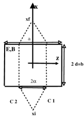
Figure 3: The particles interfere in the presence of a time-dependent electromagnetic field. The particles follow the path $C_{1}$ and $C_{2}$ in the $\mathit{x-z}$ plane as shown above for the waveguide.

Let us consider the trajectory depicted in Fig. 3. The particles are set together at one side of the pipe ($x_{\rm i}$) (at some initial time $t_{0}$), released and meet again at the other side ($x_{\rm f}$), having gone through it along straight paths. As the fields vanish outside the waveguide, the particles will interact with the electromagnetic field only when travelling inside it. Bearing in mind that $C^{d}_{\rm guide}=A^{d}_{\rm guide}+iB^{d}_{\rm guide}$, we obtain for this case

$$A^{d}_{\rm guide} = 0$$

$$B^{d}_{\rm guide} = -\frac{4}{(\omega T)^{2}-(m\pi)^{2}}|B_{0}|\frac{k_{z}}{\gamma^{2}}\sin(\frac{l\pi\alpha}{a})\bigg{[}\omega T\cos(\frac{m\pi}{2})\sin(\frac{\omega T}{2})$$ (29)

$$- m\pi\cos(\frac{\omega T}{2})\sin(\frac{m\pi}{2})\bigg{]}\bigg{(}d_{x}\omega T-m_{z}k_{z}T-2d_{y}k_{y}\bigg{)},$$

where $2d=b$ is the total distance travelled by the dipoles inside the pipe, $b$ and $a$ are the dimensions of the waveguide, $2\alpha$ is again the maximum distance the dipoles are moved apart, $m,l$ are the modes of the waveguide and $T$ the time the dipoles are travelling inside the pipe.

For the first mode of the waveguide ($l=1,m=0$), this expression looks simpler:

$$C^{d}_{\rm{TE_{10}}}=-\frac{4}{\omega T}|B_{0}|\frac{a}{\pi}\sin(\frac{\pi\alpha}{a})\sin(\frac{\omega T}{2})(d_{x}\omega T-m_{z}k_{y}T-bd_{y}k_{y}).$$ (30)

We can estimate the quantity $|C^{d}_{\rm{TE_{1,0}}}|$ in the same way we did in the preceding section, yielding

$$|C^{d}_{\rm{TE_{10}}}|\approx\frac{2\sqrt{2}}{\pi}B_{0}~{}a~{}\sin(\frac{\pi\alpha}{a})d_{x},$$ (31)

where we have assumed that $|\mathbf{d}|>>|\mathbf{m}|$. This result is independent of the dipoles’ velocity once more. Performing the same calculation with charged particles, the corresponding $|C^{e}_{\rm{TE_{10}}}|$ factor reads

$$|C^{e}_{\rm{TE_{10}}}|\approx\frac{1}{(2\pi^{3})^{1/2}}eB_{0}a\lambda v\sin\big{(}\frac{\alpha\pi}{a}\big{)}.$$ (32)

This result, opposite to the dipoles’ one, depends on the velocity of the charged particles.

Considering the dipoles again, from Eq.(29) we can compute the decoherence factor for an arbitrary $\rm{TE}$ mode of the electromagnetic field inside the cavity, $m\neq 0$ and $l\neq 0$, assuming $2d=b$. The result is

$$C^{d}_{\rm TE}\approx-\frac{4B_{0}}{(\omega T)^{2}-(m\pi)^{2}}\frac{k_{z}}{\gamma^{2}}\sin(\frac{l\pi\alpha}{a})\bigg{[}\omega T\cos(\frac{m\pi}{2})\sin(\frac{\omega T}{2})-m\pi\cos(\frac{\omega T}{2})\sin(\frac{m\pi}{2})\bigg{]}$$

$$\bigg{(}d_{x}\omega T-m_{z}k_{z}T-bd_{y}k_{y}\bigg{)}\sin(\omega t_{0}).$$ (33)

It is easy to prove that the result is negligible in the case of odd $m$ and $m\pi\ll\omega T$. In any other case we get

$$|C_{\rm TE}^{d}|\approx B_{0}a|\sin(\frac{\pi\alpha}{a})|\bigg{[}d_{x}^{2}+(\frac{b}{\omega T}d_{y}k_{z})^{2}-\frac{2b}{\omega T}d_{x}d_{y}k_{y}\bigg{]}^{1/2},$$ (34)

which has the same magnitude than for the lowest $\rm{TE}_{10}$ mode Eq.(31).

For the TM modes, the fields inside the pipe are

$$B_{x} = \frac{i\omega k_{z}}{\gamma^{2}}E_{0}\cos(k_{x}x)\cos(k_{z}z)\exp(i(k_{y}y-\omega t)),$$

$$B_{z} = \frac{-i\omega k_{x}}{\gamma^{2}}E_{0}\sin(k_{z}z)\cos(k_{x}x)\exp(i(k_{y}y-\omega t)),$$

$$E_{x} = \frac{ik_{y}k_{x}}{\gamma^{2}}E_{0}\cos(k_{x}x)\sin(k_{z}z)\exp(i(k_{y}y-\omega t)),$$

$$E_{y} = E_{0}\sin(k_{x}x)\sin(k_{z}z)\exp(i(k_{y}y-\omega t)),$$

$$E_{z} = \frac{ik_{y}k_{z}}{\gamma^{2}}E_{0}\sin(k_{x}x)\cos(k_{z}z)\exp(i(k_{y}y-\omega t)).$$ (35)

where $E_{0}=|E_{0}|\exp(i\omega t_{0})$. After some algebra, it is possible to show that

$$C^{d}_{\rm TM}=\frac{-4}{(\omega T)^{2}-(m\pi)^{2}}|E_{0}|\sin(\frac{l\pi\alpha}{a})\bigg{[}k_{x}\bigg{(}\omega T\cos(\frac{m\pi}{2})\sin(\frac{\omega T}{2})$$

$$-m\pi\cos(\frac{\omega T}{2})\sin(\frac{m\pi}{2})\bigg{)}\bigg{(}-d_{x}\frac{k_{y}}{\gamma^{2}}T+m_{z}\frac{\omega}{\gamma^{2}}T+bd_{y}\frac{\omega}{\gamma^{2}}\bigg{)}+$$

$$\bigg{(}\omega T\cos(\frac{\omega T}{2})\sin(\frac{m\pi}{2})-m\pi\cos(\frac{m\pi}{2})\sin(\frac{\omega T}{2})\bigg{)}\bigg{(}-d_{y}T-bm_{z}\bigg{)}\bigg{]}\sin(\omega t_{0}).$$ (36)

Using the same arguments than in the TE case, we can check that there is also a contribution independent of the dipoles’ velocity but this time proportional to $m_{z}$. Therefore, as we are assuming $|\mathbf{m}|<<|\mathbf{d}|$ all along this work, we conclude that $|C_{\rm TM}^{d}|\ll|C_{\rm TE}^{d}|$.

It is worth noting that in the TM case, as there is no component of the magnetic field along the guide axis, the AB phase vanishes. Therefore, the effect for neutral particles is the only one we expect.

IV Numerical estimations

When we compared the decoherence factors for charged and neutral particles (see for example Eq.(19)), we had assumed that the relevant parameters (velocity, maximum separation) were the same in both cases. Even though it is a valid thread of thought, it is not a realistic one. Therefore, in this section we will estimate the loss of coherence in more realistic situations.

In interference experiments with electrons, the wave packets can be moved apart up to $100\mu\rm{m}$ hasselbach . A typical non relativistic velocity is $v_{e}\sim 0.1$. This yields a relation $\omega T\sim 10$ for a field that has a wavelength of about $100\mu\rm{m}$. On the other hand, in atomic interferometry, two neutral particles can be separated up to $1~{}\rm{mm}$ keith ; pfau . Typical speeds are of the order $v_{d}\sim 10^{-5}$ green . We will assume the dimensions of the pipe $a\sim\rm{cm}$.

The energy density of the electromagnetic field is defined as $\rho_{\rm wave}=E_{0}^{2}/2$ for a plane wave. The energy density for the field inside a waveguide is $\rho_{\rm guide}=(aB_{0})^{2}/\lambda^{2}$. Considering the typical values of $\lambda$ and $a$ given above, we note that $a/\lambda\sim 1$ for dipoles whereas $a/\lambda\sim 10$ for electrons. As we we are using Lorentz Heaviside units with $\hbar=c=1$, $\rho$ is also the energy flux in the electromagnetic wave. We will assume an energy flux of 10 $\rm{Watts}/\rm{cm}^{2}$, approximately.

With all these values, we can estimate the $C$ factor for all the cases presented in the previous sections. The results are summarized in Table 1. As we can see, all the results for electrons are of order one or bigger, which means that the effect is experimentally observable. Dipoles’ results are smaller but not that much as one would naively expect.

Trajectories	Electrons	Dipoles
$~{}~{}|C|~{}~{}~{}$	$1$	$10^{-6}$
$|C_{\rm ellip}|~{}$	$10$	$10^{-3}$
$|C_{\rm asym}|~{}$	$10$	$10^{-1}$
$|C_{\rm{TE_{1,0}}}|$	$1$	$10^{-1}$

Table 1: Order of magnitude of the absolute value of the C factor for all trajectories, for both dipoles and electrons.

In electron’s interference experiments, we conclude that the best experimental setup would be either the asymmetric trajectory or the elliptic path. In those configurations, for adequate parameters of the trajectories it is in principle possible to obtain a complete destruction of the interference pattern (setting the value of $|C|$ equal to a zero of the Bessel function $J_{0}$). In an interference experiment with dipoles, the best experimental setup would be either the asymmetric trajectory or the waveguide. In these cases, the effect is non negligible thanks to the fact that the $C$ factor is independent of the velocity. Moreover, as shown in the Appendix, one is allowed to increase the intensity of the external field, since the scattering cross section for dipoles is much lower than for electrons, being still possible to neglect the direct interaction with the electromagnetic field.

V Final Remarks

We have estimated the loss of contrast produced when interfering particles are shined by a classical electromagnetic field. We considered both a monochromatic, linearly polarized electromagnetic field, and electromagnetic fields inside a waveguide. We considered different trajectories for both charged particles and dipoles. Symmetric and asymmetric paths have been used in order to illustrate the dependence of the fluctuating phase upon the velocity. We have shown examples (asymmetric trajectories, waveguide) in which the loss of contrast for dipoles is independent of the velocity in the low velocity limit. This particular behaviour does not show up for charged particles. However, we have found that the effect for electrons is in general larger than the one computed in Ref. ford for a particular symmetric trajectory.

We also estimated the backreaction effect of the fields over the dipoles, evaluating the scattering cross section. When the mean free path for dipoles is much larger than the characteristic dimensions of their trajectories, the direct interaction between dipoles and photons can be neglected. This condition puts an upper bound over the external field intensity. Given an external field, the decoherence for dipoles is smaller than the one expected for electrons. However, as the scattering cross section is also smaller, it is in principle possible to increase the intensity of the external fields in order to partially compensate the difference, still within the upper bound mentioned above.

Finally, we estimated the magnitude of the effect for values of the different parameters achievable in the laboratory. In the case of electrons, for an adequate setup the interference fringes can dissappear totally. For dipoles, the independence with the velocity makes the effect much more important than naively expected, and could be observed for sufficiently strong external fields.

VI Appendix

The loss of contrast computed in the previous sections depends on the intensity of the classical electromagnetic field. In the usual AB and AC effects, the force on the charges and dipoles vanishes. However, in the time dependent case considered in this paper, the dipoles have a direct interaction with the electromagnetic field, which we neglected. Therefore the intensity of the electromagnetic field is limited by the scattering cross section: the mean free path for dipoles should be much larger than the characteristic size of its trajectory.

In this section we will evaluate the scattering cross section for both dipoles in interaction with a plane wave, and dipoles travelling inside the waveguide, and compare these with the results for charged particles.

1. Plane Wave. The force experienced by a non-relativistic neutral atom with arbitrary electric and magnetic dipole moments in the presence of an electromagnetic field is schwinger

   $$\mathbf{F}=\mathbf{\nabla}\bigg{[}\mathbf{d}\cdot\mathbf{E}(\mathrm{R})+\mathbf{m}\cdot\mathbf{B}(\mathrm{R})\bigg{]}+\partial_{t}\big{(}\mathbf{d}\times\mathbf{B}(\mathrm{R})\big{)},$$ (37)

   where $\mathrm{R}$ is the position of the center of mass of the atom.

   For the plane wave of Section II, the force on the particle reads

   $$\mathbf{F}=-k_{y}E_{0}\cos(\omega t-k_{y}y)(d_{y}~{}\hat{z}+m_{x}~{}\hat{y}).$$ (38)

   If the atom’s center of mass is oscillating around the origin of coordinates ($y=0$), we can approximate the force it feels as the force evaluated at $y=0$ for every time $t$. In the non-relativistic limit, the acceleration of the particle is $\ddot{\mathbf{x}}=\mathbf{F}/m_{\rm A}$. Writing the dipole moment as $\mathbf{d}=e\mathbf{x}$, we can compute $\mathbf{\ddot{d}}$ from the force, and use Larmor’s formula to know the angular distribution of radiated power $\frac{\mathbf{d}P}{d{\mathbf{\Omega}}}=(1/4\pi)|\mathbf{\ddot{d}}|^{2}\sin^{2}(\Theta)$, where $\Theta$ is the angle between $\mathbf{\ddot{d}}$ and $\mathbf{n}$, a unit vector. The scattering cross section, averaged in time, is therefore

   $$\sigma_{d}=\frac{8\pi}{3}\frac{e^{2}}{m_{\rm A}^{2}}k_{y}^{2}(d_{y}^{2}+m_{x}^{2}).$$ (39)

   We can compare this result with Thomson’s scattering cross section $\sigma_{e}=\frac{8\pi}{3}(\frac{e^{2}}{m_{e}})^{2}$ for the case of a non-relativistic electron interacting with a plane wave. If we consider that $|d_{y}|>|m_{x}|$, then:

   $$\sigma_{d}\approx\sigma_{e}(\frac{L}{\lambda})^{2}(\frac{m_{e}}{m_{\rm A}})^{2},$$ (40)

   where $L$ is the dipole’s characteristic length and $\lambda$ is the wavelength of the field. Thus, we can see that the mean free path for dipoles $l_{\rm mfp}^{d}\sim 1/\sigma_{d}$ is bigger than the corresponding $l_{\rm mfp}^{e}$ for electrons in a factor $(\lambda/L)^{2}(m_{\rm A}/m_{e})^{2}$.

   Based on this simple observation, we conclude that the suppression of fringe visibility in the experiment done with coherent electrons or with coherent dipoles could have a similar order of magnitude. Indeed, although for a given external field the suppression is bigger for electrons than for dipoles, in the latter case it is possible to increase the intensity of the external field to partially compensate the difference, still within the limit of negligible direct interaction.

2. Waveguide. For the case of a dipole interacting with the fields of the TE mode inside a waveguide the force is written as:

   $$\mathbf{F}_{d}=\frac{kk_{z}}{\gamma^{2}}B_{0}\bigg{[}d_{x}k_{x}\sin(k_{x}x)\sin(k_{z}z)\sin(k_{y}y-\omega t)-d_{y}k_{y}\cos(k_{x}x)\sin(k_{z}z)\cos(k_{y}y-\omega t)$$

   $$-d_{z}k_{z}\cos(k_{z}z)\cos(k_{x}x)\sin(k_{y}y-\omega t)\bigg{]}\hat{x}+\frac{kk_{x}}{\gamma^{2}}B_{0}\bigg{[}d_{x}k_{x}\cos(k_{x}x)\cos(k_{z}z)\sin(k_{y}y-\omega t)$$

   $$+d_{y}k_{y}\sin(k_{x}x)\cos(k_{z}z)\cos(k_{y}y-\omega t)-d_{z}k_{z}\sin(k_{x}x)\sin(k_{z}z)\sin(k_{y}y-\omega t)\bigg{]}\hat{z}$$ (41)

   Following the reasoning above for the case of the plane wave, we obtain that the scattering cross section of the TE mode is given by

   $$\sigma_{\rm TE}^{d}\approx\frac{8\pi}{3}\frac{e^{2}d_{y}^{2}}{m_{\rm A}^{2}}kk_{y}=\frac{8\pi}{3}\frac{e^{4}}{m_{\rm A}^{2}}L^{2}kk_{y}=\sigma_{\rm TE}^{e}k_{y}^{2}L^{2}(\frac{m_{e}}{m_{\rm A}})^{2}$$ (42)

   where $\sigma_{\rm TE}^{e}=\frac{8\pi}{3}\frac{e^{4}}{m_{e}^{2}}\frac{k}{k_{y}}$ is the total cross section for an electron inside the waveguide in the TE mode (for simplicity we assumed that $k_{x}\sim k_{z}$, and $a\sim b$). Therefore, we obtain $\sigma_{\rm TE}^{d}\ll\sigma_{\rm TE}^{e}$, and $l_{\rm mfp}^{d,\rm TE}\gg l_{\rm mfp}^{e,\rm TE}$

   For the TM modes, an analogous calculation shows that $\sigma_{\rm TM}^{d}\approx\sigma_{\rm TE}^{d}$.

VII Acknowledgments

We thank Juan Pablo Paz for useful discussions. This work was supported by UBA, CONICET, Fundación Antorchas, and ANPCyT, Argentina.

References

- (1) Y. Aharonov and D.Bohm, Phys. Rev. 115, 485 (1959).
- (2) A. Stern, Y. Aharonov, and Y. Imry, Phys. Rev. A41, 3436 (1990).
- (3) F.D. Mazzitelli, J.J. Paz, and A. Villanueva, Phys. Rev. A68, 062106 (2003).
- (4) C.C. Chong, D.I. Tsomokos, and A. Vourdas, Phys. Rev. A66, 033813 (2002). See also: D.I. Tsomokos, C.C. Chong, and A. Vourdas, quant-ph/0502113.
- (5) D.I. Tsomokos, C.C. Chong, and A. Vourdas, Phys. Rev. A69, 03810 (2004).
- (6) A. Vourdas, Phys. Rev. A64, 053814 (2001).
- (7) Jen-Tsung Hsiang and L.H.Ford, Phys. Rev. Lett. 25, 250402 (2004).
- (8) Y. Aharonov and A. Casher, Phys. Rev. Lett. 53, 319 (1984).
- (9) K. Sangster, E. Hinds, S. Barnett, E. Riis, and A. Sinclair, Phys. Rev. A51, 1776 (1995).
- (10) J. Anandan, Phys. Rev. Lett. 85, 1354 (2000).
- (11) M.V. Berry, Proc. Soc. London Ser. A392, 45 (1991).
- (12) Y. Aharonov, S.A. Pearle, and L. Vaidman, Phys. Rev. A37, 4052 (1988).
- (13) G. Spavieri, Phys. Rev. Lett. 82, 3932 (1999).
- (14) A. Cimmino, G.I. Opat, A.G. Klein, H. Kaiser, S.A. Wermer, M. Arif, and R. Clothier, Phys. Rev. Lett. 63, 380 (1989).
- (15) K. Sangster, E. Hinds, S. Barnett, and E. Riis, Phys. Rev. Lett. 71, 3641 (1993).
- (16) J. Schwinger, L. L. DeRaad, K. Milton, and W. Tsai, Classical Electrodynamics, Advanced Book Program, Westview Press, 1998.
- (17) F. Hasselbach, Z. Phys. B: Condens. Matter 71, 443 (1988).
- (18) D. W. Keith et al., Phys. Rev. Lett. 66, 2693 (1991).
- (19) T. Pfau et al., Phys. Rev. Lett. 71, 3427 (1993).
- (20) D. M. Greenberger, D. K. Atwood, J. Arthur, C. G. Shull, and M. Schlenker, Phys. Rev. Lett. 47, 751 (1981).