Witnessing Entanglement of EPR States With
Second-Order Interference

Abstract

The separability of the continuous-variable EPR state can be tested with Hanbury-Brown and Twiss type interference. The second-order visibility of such interference can provide an experimental test of entanglement. It is shown that time-resolved interference leads to the Hong, Ou and Mandel deep, that provides a signature of quantum non-separability for pure and mixed EPR states. A Hanbury-Brown and Twiss type witness operator can be constructed to test the quantum nature of the EPR entanglement.

1 Introduction

The famous debate between Einstein, Podolsky, Rosen (EPR) and Bohr [1, 2], about the nature of quantum correlations of a bi-partite state has played a key role in the investigation of entanglement properties of light in modern Quantum Optics, and has initiated a new branch of physics called Quantum Information. EPR used in their arguments a wave function that exhibits a perfect correlations between positions and momenta of two massive particles (labeled $a$ and $b$). In the position and momentum representations the EPR state takes the following forms

$$\Psi(x_{a},x_{b})\simeq\delta(x_{a}-x_{b}),\quad\widetilde{\Psi}(p_{a},p_{b})\simeq\delta(p_{a}+p_{b}).$$ (1)

Quantum correlations of the entangled EPR state have been implemented experimentally for massless particles: photons. In the case of light, the quantum mechanical position and momentum observables are played by the electric field: phase and amplitude quadratures.

The well known two-mode Gaussian squeezed states of light are physical realization of the EPR state. Those states lie at the heart of quantum cryptography [crypt], quantum information [4] and quantum teleportation [5].

There are few efficient ways of producing Gaussian EPR correlated states. One of them uses a Kerr nonlinear medium in optical fibers to entangle phase and amplitude quadratures [6]. However, the nonlinearity has to be relatively small to achieve a Gaussian state. The other method uses a beam splitter as a nonlocal operation that creates entanglement. A typical setup consists of two initially separable amplitude squeezed beams which interfere at the 50/50 beam splitter.

Recent applications of entangled two-mode squeezed states of light in quantum information processing have generated a lot of interest in mixed Gaussian states. Although there are mathematical criterions for the entangled properties for mixed two-partite Gaussian systems [7], they are not easy experimentally realizable.

It is the purpose of this paper to show that Hanbury-Brown and Twiss (HBT) interference can reveal the quantum nature of entanglement of two-particle mixed Gaussian states. We show that it is possible to construct a quantum witness operator, closely related to the HBT interference [8], that probe entanglement of a mixed EPR Gaussian state. Using Hong, Ou and Mandel (HOM) interferometry we discuss the entangled properties of time resolved interference of the EPR state. We show that the deep in HOM interference can provide a useful tool to study quantum separability of continuous-variable Gaussian EPR states.

2 Mixed EPR states

A non-degenerated optical parametric amplification, involving two modes of the radiation field, provides a physical realization of the EPR state (1). The quantum state generated in this process has the following form

$$|\Psi\rangle=\sum_{n=0}^{\infty}\,\sqrt{p_{n}}\,|n,n\rangle,$$ (2)

where $p_{n}=\bar{n}^{n}/(1+\bar{n})^{n+1}$ is a thermal distribution with a mean number $\bar{n}$ of photons in each mode.

Using field quadratures eigenstates: $|x_{a},x_{b}\rangle$, we obtain that the wave function of such a system (2) is Gaussian and has the form

$$\langle x_{a},x_{b}|\Psi\rangle=\frac{1}{\sqrt{\pi}}e^{-(\bar{n}+\frac{1}{2})(x_{a}^{2}+x_{b}^{2})+2\sqrt{\bar{n}(1+\bar{n})}x_{a}x_{b}}\,.$$ (3)

In the limit of $\bar{n}\rightarrow\infty$, the two-mode squeezed state (3) becomes the original EPR state (1). The state (3) is not entangled only if $\bar{n}=0$.

The simplest mixed generalization of the EPR state involves a Gaussian density operator $\rho_{ab}$, being a Gaussian operator of the field modes described by the annihilation and creation operators $(a,a^{\dagger})$ and $(b,b^{\dagger})$. This Gaussian density operator of the two modes is fully characterized by its second moment expectation values of the modes. In the case of a mixed EPR state the only non-vanishing field correlations are

$$\langle a^{\dagger}a\rangle=\langle b^{\dagger}b\rangle=\bar{n},\ \ \langle ab\rangle=-m_{c},$$ (4)

where $\bar{n}$ is a mean number of photons in each mode, and $m_{c}$ correspond to the amount of correlation between the two modes. For $|m_{c}|=\sqrt{\bar{n}(\bar{n}+1)}$, the EPR state reduces to the pure state given by (3).

As it has been discussed in several papers (see the tutorial [7] and references therein), this mixed EPR state is separable for $\bar{n}>|m_{c}|$ and its density operator can be expressed in a sum of product states (Werner separability criterion)

$$\rho_{\mathrm{ab}}=\sum_{i}p_{i}\,\rho^{i}(a)\otimes\rho^{i}(b),$$ (5)

where $\rho^{i}(a)$, $\rho^{i}(b)$ are the density operators of the two modes and $\sum_{i}p_{i}=1$, with $0\leq p_{i}\leq 1$. The mixed EPR state is entangled and non-separable if

$$\bar{n}<|m_{c}|<\sqrt{\bar{n}(\bar{n}+1)}\,.$$ (6)

3 Hanbury-Brown and Twiss Interference with EPR Pairs

Second and higher orders of coherence of a light beam can reveal its quantum nature, which cannot be observed in Young-type interference experiments. Second-order interference involving intensity-intensity correlations have been first applied by Hanbury-Brown and Twiss in stellar interferometry [9]. In modern Quantum Optics, second-order interference has been used as powerful tool to study nonclassical properties of light [10].

Hanbury-Brown and Twiss (HBT) interference measures a second-order normally ordered intensity-intensity correlation function. In Fig. 1 we have depicted a setup for HBT interference that involves two light beams with annihilation operators $a$ and $b$ interfering at the beam splitter. A correlation between clicks of two detectors corresponds to a normally ordered intensity-intensity correlation function. The HBT interference exhibits a typical pattern of the form: $1+v^{(2)}\cos(\varphi_{1}-\varphi_{2})$, where $\varphi_{1}$ and $\varphi_{2}$ are phase differences between the beams $a$ and $b$ in front of the detectors. These phases include geometrical phases and phases due to the possible action of the beam splitter. In this setup the two phases can be controlled experimentally. $v^{(2)}$ is a second-order interference visibility. For a classical source of light this visibility is always bounded: $v^{(2)}\leq\frac{1}{2}$. This classical limit is violated for single photons, as it has been shown in the pioneering experiments performed by Mandel [11].

Figure 1: Hanbury-Brown and Twiss second-order interference.

We shall apply the HBT setup to study the mixed Gaussian EPR state. At the detectors ($i=1,2$) the positive-frequency part of electric field corresponding to modes $c$ and $d$ (normalized to the number of photons) is as follows

$$E^{(+)}(\varphi_{i})=\frac{a\pm be^{i\varphi_{i}}}{\sqrt{2}}\,.$$ (7)

The corresponding field intensity operator at the screen is equal to

$$I(\varphi_{i}) = E^{(-)}(\varphi_{i})E^{(+)}(\varphi_{i})=\frac{1}{2}(a^{\dagger}a+b^{\dagger}b\pm b^{\dagger}a\,e^{-i\varphi_{i}}\pm a^{\dagger}b\,e^{i\varphi_{i}}).$$ (8)

From this expression, we obtain that the normally ordered second-order intensity correlation is

$$\langle{:}I(\varphi_{1})\,I(\varphi_{2}){:}\rangle = \frac{1}{4}\Big{[}\langle:(a^{\dagger}a+b^{\dagger}b)^{2}:\rangle-2\langle a^{\dagger}a\,b^{\dagger}b\rangle\cos(\varphi_{1}-\varphi_{2})$$ (9)

$$+ (e^{-i\varphi_{1}}-e^{-i\varphi_{2}})\langle b^{\dagger}(a^{\dagger}a+b^{\dagger}b)\,a\rangle+(e^{i\varphi_{1}}-e^{i\varphi_{2}})\langle a^{\dagger}(a^{\dagger}a+b^{\dagger}b)\,b\rangle$$

$$- e^{-i(\varphi_{1}+\varphi_{2})}\langle{b^{\dagger}}^{2}a^{2}\rangle-e^{i(\varphi_{1}+\varphi_{2})}\langle{a^{\dagger}}^{2}b^{2}\rangle\Big{]}\,.$$

For the EPR beams in a mixed state, with mean $\bar{n}$ photons and correlation $m_{c}$ described by the relations from Eq.(4), the fourth-order field correlations needed in the HBT calculations are equal to

$$\langle a^{\dagger}a^{\dagger}a\,a\rangle=2\bar{n}^{2}\,,\quad\langle b^{\dagger}b^{\dagger}b\,b\rangle=2\bar{n}^{2}\,,\,\quad\langle a^{\dagger}a\,b^{\dagger}b\rangle=\bar{n}^{2}+|m_{c}|^{2}\,.$$ (10)

As a result the HBT intensity correlation function (9), for a continuous variable mixed EPR state, has the following form

$$\langle{:}I(\varphi_{1})\,I(\varphi_{2}){:}\rangle=\frac{1}{2}(3\bar{n}^{2}+|m_{c}|^{2})\left\{1-v^{(2)}\cos(\varphi_{1}-\varphi_{2})\right\}\,,$$ (11)

with the second-order fringe visibility equal to

$$v^{(2)}=\frac{\bar{n}^{2}+|m_{c}|^{2}}{3\bar{n}^{2}+|m_{c}|^{2}}\,.$$ (12)

For a separable (classical) output state we have: $\frac{1}{3}\leq v^{(2)}\leq\frac{1}{2}$. In the case of no correlation in the output state $|m_{c}|=0$, the visibility is $v^{(2)}=\frac{1}{3}$, as it should be for a thermal state. For entangled states this visibility is quantum i.e., it violates the classical inequality: $v^{(2)}\leq\frac{1}{2}$.

In Fig. 2 and Fig. 3 we have depicted the visibility (12) as a function of the correlation parameter $m_{c}$ for two different values of $\bar{n}=1,0.1$.

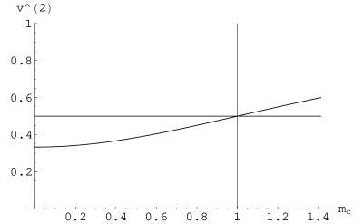
Figure 2: The visibility (12) evaluated for $\bar{n}=1$. The vertical grid line defines a border between entangled and separable EPR states. For $|m_{c}|>1$ the state is entangled and the visibility is greater than $\frac{1}{2}$ - horizontal grid line.

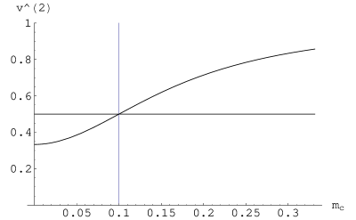
Figure 3: The visibility (12) evaluated for $\bar{n}=0.1$. The vertical grid line defines a border between entangled and separable EPR states. For $|m_{c}|>0.1$ the state is entangled and the visibility is greater than $\frac{1}{2}$ - horizontal grid line.

Based on the above visibility analysis one can introduce a HBT witness operator

$$\mathcal{W}^{(HBT)}=\frac{1}{2}-\frac{2a^{\dagger}b^{\dagger}a\,b}{\langle:(I_{a}+I_{b})^{2}:\rangle}.$$ (13)

The mean value of this operator,

$$\mathrm{Tr}\{\mathcal{W}^{(HBT)}\rho_{\mathrm{AB}}\}=\frac{\bar{n}^{2}-|m_{c}|^{2}}{2(3\bar{n}^{2}+|m_{c}|^{2})}\,,$$ (14)

is positive for separable mixed EPR states and negative for entangled mixed EPR states.

4 Hong-Ou-Mandel Time-Resolved Interference

The analysis of second-order interference, can be extended to the case of photon pulses which duration is long compared to the time resolution of photodetector. Such single-photon emitters are already in use [12, 13].

A source produces single photon pulses with a relative delay which interfere at the beam splitter. Simple analysis of beam splitter’s action on impinging photons shows, that both photons will leave the same outport of the beam splitter. A relative delay is small enough to keep the pulses partially overlapping. Even though the overlapping is not complete, its time duration is longer than the time resolution of the detector. Therefore, the temporal effects cannot be neglected any more when detecting pulses and the time delay $\tau$ between detected pulses at two separate detectors has to taken into account. Experiments investigating interference for such pulses with different frequencies have already been performed [14, 15].

We restrict our description of the single-photon wave packets in the space-time domain to one-mode fields with electric field operators: $E^{(+)}_{a}(t)=\alpha(t)\,a$ and $E^{(+)}_{b}(t)=\beta(t)\,b$. The phases $\varphi_{1}$ and $\varphi_{2}$ are included in the mode functions phases. These mode phases contain an additive stochastic component related to the random arrival time of the correlated photons at the beam splitter or detectors. The time dependent electric fields of the two-mode output state is described by the beam splitter transformation (see Eq. (7))

$$E^{(+)}_{c}(t)=\frac{E^{(+)}_{a}(t)+E^{(+)}_{b}(t)}{\sqrt{2}},\quad E^{(+)}_{d}(t)=\frac{E^{(+)}_{a}(t)-E^{(+)}_{b}(t)}{\sqrt{2}}.$$ (15)

The joint coincidence of detecting photons from mode $c$ and $d$ at delayed times $t$ and $t+\tau$ can be obtained directly from the following second-order temporal coherence function

$$G^{(2)}(t,t+\tau)=\left\langle E^{(-)}_{c}(t)\,E^{(-)}_{d}(t+\tau)\,E^{(+)}_{d}(t+\tau)\,E^{(+)}_{c}(t)\right\rangle.$$ (16)

Using the mode functions, with random phases in the output state, we note that the only contributing terms to the second-order coherence function are the following

$$G^{(2)}(t,t+\tau) = \frac{1}{4}\Big{\{}|\alpha(t)|^{2}|\alpha(t+\tau)|^{2}\;\langle a^{\dagger}a^{\dagger}a\,a\rangle+|\beta(t)|^{2}|\beta(t+\tau)|^{2}\;\langle b^{\dagger}b^{\dagger}b\,b\rangle$$ (17)

$$+ \Big{[}|\alpha(t)|^{2}|\beta(t+\tau)|^{2}+|\alpha(t+\tau)|^{2}|\beta(t)|^{2}$$

$$- \big{(}\alpha(t+\tau)\alpha^{*}(t)\beta(t)\beta^{*}(t+\tau)+\textrm{c.c.}\big{)}\Big{]}\,\langle a^{\dagger}b^{\dagger}a\,b\rangle\Big{\}}.$$

As an example we shall use in the calculations a special model of phase fluctuations. We will assume that the mode functions have random phases typical for a stationary stochastic phase diffusion model. In this example, the only non-vanishing autocorrelations of the mode functions are

$$\langle\alpha^{*}(t)\alpha(t+\tau)\rangle=I_{a}\,\exp{\left(-\frac{\tau^{2}}{\tau_{a}^{2}}\right)},\quad\langle\beta^{*}(t)\beta(t+\tau)\rangle=I_{b}\,\exp{\left(-\frac{\tau^{2}}{\tau_{b}^{2}}\right)}\,.$$ (18)

In these formulas we have assumed that the statistical correlations are stationary and Gaussian with coherence times $\tau_{a}$ and $\tau_{b}$. The stationary intensities are: $\langle\alpha^{*}(t)\alpha(t)\rangle=I_{a}$ and $\langle\beta^{*}(t)\beta(t)\rangle=I_{b}$.

Applying the above temporal correlations of the mode functions, combined with the EPR correlations of a mixed state given by Eq. (10), we obtain that the second-order coherence function is stationary (dependents only on time $\tau$) and has the form

$$G^{(2)}(\tau)=\frac{1}{2}\left\{\bar{n}^{2}\,(I_{a}^{2}+I_{b}^{2})-(\bar{n}^{2}+|m_{c}|^{2})\,I_{a}I_{b}\,\exp{\left(-\frac{\tau^{2}}{\tau_{a}^{2}}-\frac{\tau^{2}}{\tau_{b}^{2}}\right)}\right\}\,.$$ (19)

We shall simplify this formula further assuming that the mode intensities are equal: $I_{a}=I_{b}=I$. Setting $\frac{1}{\tau_{a}^{2}}+\frac{1}{\tau_{b}^{2}}=\frac{1}{\tau_{c}^{2}}$ the formula above reduces to

$$G^{(2)}(\tau) = \frac{I^{2}}{2}\,(3\bar{n}^{2}+|m_{c}|^{2})\,\left\{1-v^{(2)}\,e^{-\frac{\tau^{2}}{\tau^{2}_{c}}}\right\}\,$$ (20)

with the second-order visibility $v^{(2)}$ equal to (12). From this formula we obtain that a joint coincidence probability to detect a photon at time $t$ and another photon at time $t+\tau$ is

$$p(T)=1-v^{(2)}\,\exp{(-T^{2})}\,,$$ (21)

where $T$ is a dimensionless time with $\tau$ expressed in units of $\tau_{c}$.

This coincidence probability exhibits a typical Hong-Ou-Mandel deep [16]. In Fig. 4, we have depicted the joint coincidence probability for a state with $\bar{n}=1$. The upper curve ($\bar{n}=1$ and $|m_{c}|=1$) is a border between separable and nonseparable EPR states. The lower curve ($\bar{n}=1$ and $|m_{c}|=\sqrt{2}$) describes HOM interference of an entangled pure EPR state. The region between the two curves corresponds to nonseparable mixed EPR sates. For $\bar{n}=1$ the minimum value the HOM deep for a pure state is achieved at a zero coincident rate and is equal to $p_{min}=0.4$.

For the EPR state given by Eq. (2), with a small value of $\bar{n}$, one can get a significant increase of the the deep. For a weak two-mode pure squeezed state $(\bar{n}\ll 1)$ we can approximate the formula (2) by

$$|\Psi\rangle\sim\sqrt{p_{0}}\,|0,0\rangle+\sqrt{p_{n}}\,|1,1\rangle\,.$$ (22)

We see that such a weak pure squeezed state is the same as the one discussed in the single photon experiment originally performed by HOM [16].

Fig. 5 illustrates the HOM deep for a state with $\bar{n}=0.1$. The upper curve ($\bar{n}=0.1$ and $|m_{c}|=0.1$) is a border between separable and nonseparable EPR states. The lower curve ($\bar{n}=0.1$ and $|m_{c}|=\sqrt{0.11}$) describes HOM interference of an entangled pure EPR state approximated by the state exhibited above. The region between the two curves corresponds to nonseparable mixed EPR sates. For $\bar{n}=0.1$ the minimum value the HOM deep for a pure state is achieved at a zero coincident rate and is equal to $p_{min}=0.14$.

Figure 4: The plots of joint coincidence probability $p(T)$ as a function of $T$ for pure (the lower curve) and mixed separable (the upper curve) EPR states are depicted. The minimum value of $p(T)$ for the pure state ($\bar{n}=1$ and $|m_{c}|^{2}=2$) is below $\frac{1}{2}$. For a mixed state from the border between entangled and separable states, ($\bar{n}=1$ and $|m_{c}|^{2}=1$), $p(T)$ reaches the value of $\frac{1}{2}$ but does not exceed it.

Figure 5: Similarly, as in Fig. 4, for a state with $\bar{n}=0.1$, probability $p(T)$ exceeds the value of $\frac{1}{2}$ for a pure state ($|m_{c}|^{2}=0.11$, the lower curve). In this case the minimum value is smaller than for $\bar{n}=1$ and reaches $0.14$. For the border state, between entangled and separable states ($|m_{c}|^{2}=0.01$, the upper curve), the minimum value of $p(T)$ is again equal to $\frac{1}{2}$.

5 Conclusions

In this paper we have shown that the Hanbury-Brown and Twiss type interference can be used as an experimental test of quantum separability for continuous variable EPR states. One can associate with this second-order interference a HBT witness operator quantifying entanglement for pure and mixed Gaussian EPR states. We have shown that time-resolved coincidence rate of joint photon detection exhibits the Hong, Ou and Mandel deep, that provides a signature of quantum nonseparability for pure and mixed EPR states.

References

- [1] A. Einstein, B. Podolsky, N. Rosen, Phys. Rev. 47, 777, (1935).
- [2] N. Bohr, Phys. Rev. 48, 698, (1935).
- [3] A. K. Ekert, J. G. Rarity, P. R. Tapster, and G. M. Palma, Phys. Rev. Lett. 69, 1293 (1992).
- [4] S. L. Braunstein and A. K. Pati, (eds), Quantum Information Theory with Continuous Variable, (Kulwer, Dordrecht, 2002).
- [5] A. Furusawa et al., Science 282, 706 (1998).
- [6] Ch. Silberhorn, P.K. Lam, O. Weiß, F. König, N. Korolkova, and G. Leuchs, Phys. Rev. Lett. 86, 4267 (2001).
- [7] See for example the tutorial: B.-G. Englert and K. Wódkiewicz, International Journal of Quantum Information 1, 153, (2003), and references therein.
- [8] M. Stobińska, K. Wódkiewicz, Phys. Rev. A 71, 032304 (2005).
- [9] R. Hanbury-Brown and R. Q. Twiss, Nature 127, 27, (1956).
- [10] M. O. Scully and M. S. Zubairy, Quantum Optics, (Cambridge University Press, 2002).
- [11] L. Mandel, Rev. Mod. Phys. 71, 274, (1999).
- [12] A. Kuhn, M. Hennrich, G. Rempe, Phys. Rev. Lett. 89, 067901, (2002).
- [13] A. Kuhn, M. Hennrich, G. Rempe, Quantum Information Processing, (Wiley-VCH, Berlin 2003).
- [14] T. Legero, T. Wilk, M. Hennrich, G. Rempe, and A. Kuhn, Phys. Rev. Lett. 93, 070503, (2004).
- [15] T. Legero, T. Wilk, A. Kuhn, G. Rempe, Appl. Phys. B, (2003).
- [16] C. K. Hong, Z. Y. Ou, L. Mandel, Phys. Rev. Lett. 59, 2044, (1987).