Abstract

In the formalism of measurement based quantum computation we start with a given fixed entangled state of many qubits and perform computation by applying a sequence of measurements to designated qubits in designated bases. The choice of basis for later measurements may depend on earlier measurement outcomes and the final result of the computation is determined from the classical data of all the measurement outcomes. This is in contrast to the more familiar gate array model in which computational steps are unitary operations, developing a large entangled state prior to some final measurements for the output. Two principal schemes of measurement based computation are teleportation quantum computation (TQC) and the so-called cluster model or one-way quantum computer (1WQC). We will describe these schemes and show how they are able to perform universal quantum computation. We will outline various possible relationships between the models which serve to clarify their workings. We will also discuss possible novel computational benefits of the measurement based models compared to the gate array model, especially issues of parallelisability of algorithms.

1 Introduction

Many of the most popular models of quantum computation are direct quantum generalisations of well known classical constructs. This includes quantum turing machines, gate arrays and walks. These models use unitary evolution as the basic mechanism of information processing and only at the end do we make measurements, converting quantum information into classical information in order to read out classical answers. In contrast to unitary evolution, measurements are irreversibly destructive, involving much loss of potential information about a quantum state’s identity. Thus it is interesting, and at first sight surprising, that we can perform universal quantum computation using only measurements as computational steps [2, 3, 4, 5, 6]. These “measurement based” models are especially interesting for fundamental issues: they have no evident classical analogues and they offer a new perspective on the role of entanglement in quantum computation. They may also be interesting for experimental considerations, suggesting a different kind of computer architecture and offering interesting possibilities for further issues such as fault tolerance [7].

We will discuss two measurement based models. Firstly we’ll consider teleportation quantum computation (TQC). This is based on the idea of Gottesman and Chuang [2] of teleporting quantum gates, and was developed into a computational model by Nielsen, Leung and others [3, 4]. Secondly we will consider the so-called “one way quantum computer” (1WQC) or “cluster state computation” of Raussendorf and Briegel [5, 6]. Then we will discuss various possible relationships between these two models and finally consider possible computational benefits of the measurement based formalism as compared to the quantum gate array model.

The following notations will be frequently used. The Pauli operators are

$$I=\left(\begin{array}[]{rr}1&0\\ 0&1\end{array}\right)\hskip 8.53581ptX=\left(\begin{array}[]{rr}0&1\\ 1&0\end{array}\right)\hskip 8.53581ptZ=\left(\begin{array}[]{rr}1&0\\ 0&-1\end{array}\right)\hskip 8.53581ptiY=ZX=\left(\begin{array}[]{rr}0&1\\ -1&0\end{array}\right).$$

$\oplus$ will denote addition modulo 2. The controlled-NOT gate $CX$ is defined by

$$CX\left|i\right\rangle\left|j\right\rangle=\left|i\right\rangle\left|i\oplus j\right\rangle\hskip 14.22636pti,j=0,1.$$

The controlled phase gate $CZ$ is defined by

$$CZ\left|i\right\rangle\left|j\right\rangle=(-1)^{ij}\left|i\right\rangle\left|j\right\rangle.$$

In contrast to the $CX$ gate, $CZ$ is symmetrical in the two input qubits. The Hadamard operator is

$$H=\frac{1}{\sqrt{2}}\left(\begin{array}[]{rr}1&1\\ 1&-1\end{array}\right)$$

and the Hadamard basis states are

$$\left|\pm\right\rangle=\frac{1}{\sqrt{2}}(\left|0\right\rangle\pm\left|1\right\rangle).$$

The Bell basis states are

$$\begin{array}[]{l}\left|B_{00}\right\rangle=\frac{1}{\sqrt{2}}(\left|00\right\rangle+\left|11\right\rangle)=I\otimes I\left|B_{00}\right\rangle\\ \left|B_{01}\right\rangle=\frac{1}{\sqrt{2}}(\left|01\right\rangle+\left|10\right\rangle)=X\otimes I\left|B_{00}\right\rangle\\ \left|B_{10}\right\rangle=\frac{1}{\sqrt{2}}(\left|00\right\rangle-\left|11\right\rangle)=Z\otimes I\left|B_{00}\right\rangle\\ \left|B_{11}\right\rangle=\frac{1}{\sqrt{2}}(\left|01\right\rangle-\left|10\right\rangle)=iY\otimes I\left|B_{00}\right\rangle.\\ \end{array}$$

Succinctly we have

$$\left|B_{cd}\right\rangle=Z^{c}X^{d}\otimes I\left|B_{00}\right\rangle.$$

We will also use the maximally entangled state that combines the Hadamard and standard bases in its Schmidt form:

$$\left|H\right\rangle=\frac{1}{\sqrt{2}}\left(\left|0\right\rangle\left|+\right\rangle+\left|1\right\rangle\left|-\right\rangle\right)=\frac{1}{\sqrt{2}}\left(\left|+\right\rangle\left|0\right\rangle+\left|-\right\rangle\left|1\right\rangle\right)=CZ\left|+\right\rangle\left|+\right\rangle.$$

2 Teleportation based quantum computing

Recall standard teleportation [1] as depicted in figure 1 and explained in the caption.

Figure 1: Standard quantum teleportation. The labels 1,2,3 represent three qubits. 1 is in state $\left|\alpha\right\rangle$ and 23 are in state $\left|B_{00}\right\rangle$. A Bell measurement is performed on 12. If the outcome is $\left|B_{cd}\right\rangle$ then qubit 3 acquires the state $X^{d}Z^{c}\left|\alpha\right\rangle$.

Now introduce the “rotated Bell basis” denoted ${\cal B}(U)=\{\left|B(U)_{cd}\right\rangle\}$ where for any 1-qubit gate $U$:

$$\left|B(U)_{cd}\right\rangle=U^{\dagger}\otimes I\left|B_{cd}\right\rangle.$$

A simple calculation shows that if we perform such a rotated Bell measurement (instead of the standard one in figure 1) then the teleported state at 3 is $X^{d}Z^{c}U\left|\psi\right\rangle$ i.e. the gate $U$ has been applied to $\left|\psi\right\rangle$ via this teleportation [2]. A particularly neat and general way of performing this calculation is the following. For any dimension $d$ consider any maximally entangled state, written in its Schmidt form as

$$\left|\phi\right\rangle=\frac{1}{\sqrt{d}}\sum_{i=0}^{d-1}\left|i\right\rangle\left|i\right\rangle.$$

Consider the mathematical projection depicted in figure 2.

Figure 2: Projecting the three qubit state $\left|\alpha\right\rangle_{1}\left|\phi\right\rangle_{23}$ onto the maximally entangled state $\left|\phi\right\rangle_{12}$ results in a single qubit state at 3 given by $\frac{1}{d}\left|\alpha\right\rangle_{3}$ (see lemma 1).

Lemma 1:   The projection of $\left|\alpha\right\rangle_{1}\left|\phi\right\rangle_{23}$ onto $\left|\phi\right\rangle_{12}$ results in the state $\frac{1}{d}\left|\alpha\right\rangle_{3}$ at qubit 3.

Proof:   Let $\left|\alpha\right\rangle=\sum a_{j}\left|j\right\rangle$. Then the projection is

$$\frac{1}{d}(\sum_{i}\left\langle i\right|\left\langle i\right|)(\sum_{jk}a_{j}\left|j\right\rangle\left|k\right\rangle\left|k\right\rangle)=\frac{1}{d}\sum_{ijk}a_{j}\delta_{ij}\delta_{ik}\left|k\right\rangle=\frac{1}{d}\sum_{k}a_{k}\left|k\right\rangle.\hskip 14.22636pt\Box$$

Next introduce the “rotated $\left|\phi\right\rangle$ state”: for any unitary operator $U$ in $d$ dimensions define

$$\left|\phi(U)\right\rangle=U^{\dagger}\otimes I\left|\phi\right\rangle.$$ (1)

Lemma 2:   The projection of $\left|\alpha\right\rangle_{1}\left|\phi\right\rangle_{23}$ onto $\left|\phi(U)\right\rangle_{12}$ results in the state $\frac{1}{d}U\left|\alpha\right\rangle_{3}$ at qubit 3.

Proof:   For any states $\left|a\right\rangle$, $\left|b\right\rangle$ if we write $\left|U^{\dagger}a\right\rangle=U^{\dagger}\left|a\right\rangle$ then $\left\langle U^{\dagger}a|b\right\rangle=\left\langle a|Ub\right\rangle$. Hence lemma 1 with $\left|\phi\right\rangle_{12}$ replaced by $\left|\phi(U)\right\rangle_{12}$ immediately gives the result.$\Box$

Now the basic idea is to regard the 12-projections in lemmas 1 and 2 as being outcomes of a projective measurement applied to qubits 1 and 2 i.e. we wish to choose a set of $d^{2}$ unitaries $U_{i}$ such that $\{\left|\phi(U_{i})\right\rangle\}$ form an orthonormal basis of the 12 space. For qubits ($d=2$) the set $\{I,X,Z,XZ\}$ gives standard teleportation and the set $\{IU,XU,ZU,XZU\}$ gives the rotated Bell basis, reproducing our previous procedure of “gate teleportation” to construct $X^{d}Z^{c}U\left|\psi\right\rangle$ at qubit 3.

Note that lemmas 1 and 2 apply in general dimension $d$ so we can apply 2-qubit gates such as $CZ$ via measurements by teleportation in dimension $d=4$. For example using $\left|\phi\right\rangle=\left|B_{00}\right\rangle\left|B_{00}\right\rangle$ and the 16 operators $U_{ij}=(P_{i}\otimes P_{j})CZ$ where $P_{i}$ and $P_{j}$ range over the four standard Pauli operators, we can check that $\{U_{ij}^{\dagger}\otimes I\left|\phi\right\rangle\}$ is an orthonormal set and the output teleported state is $(P_{i}\otimes P_{j})CZ\left|\psi\right\rangle$ for any input 2-qubit state $\left|\psi\right\rangle$.

This method of applying $CZ$ requires a 16 dimensional Bell measurement but with more subtle means we can achieve the result with smaller measurements. An illustrative example (taken from [18]) is shown in figure 3.

Figure 3: Application of $CZ$ by teleportation with 8 dimensional measurements. The wiggly line connecting 12 denotes an input 2-qubit state $\left|\psi\right\rangle$. The lines labelled $H$ denote the maximally entangled state $\left|H\right\rangle$. Introduce the 3-qubit Bell measurement corresponding to the basis $\{\left|000\right\rangle\pm\left|111\right\rangle,\left|001\right\rangle\pm\left|110\right\rangle,\left|010\right\rangle\pm\left|101\right\rangle,\left|100\right\rangle\pm\left|011\right\rangle\}$. If this measurement is performed on qubits 135 and 246 then it can be verified that qubits 78 acquire the state $(P_{i}\otimes P_{j})(H\otimes H)CZ\left|\psi\right\rangle$ where the Pauli operators $P_{i}$ and $P_{j}$ depend on the measurement outcomes.

Remark:    Returning to $\left|\phi(U)\right\rangle$ in eq. (1), a set of $d^{2}$ operators $\{U_{i}\}$ will have the corresponding set $\{\left|\phi(U_{i})\right\rangle\}$ being orthonormal iff $\mbox{Tr}\,(U_{i}U^{\dagger}_{j})=\delta_{ij}$ i.e. $\{U_{i}\}$ is a so-called unitary operator basis. For general dimension $d$ many such sets exist, each corresponding to a teleportation scheme. Werner [8] has described a method for constructing a large number of explicit inequivalent examples. However we can go even further and choose a set of $n\geq d^{2}$ operators $U_{i}$ such that the set $\{k_{i}\left|\phi(U_{i})\right\rangle\left\langle\phi(U_{i})\right|\}$ (for some chosen constants $k_{i}>0$) form the elements of a (rank 1) positive operator valued measure (POVM) i.e. we ask that

$$\sum_{i=1}^{n}k_{i}\left|\phi(U_{i})\right\rangle\left\langle\phi(U_{i})\right|=I_{d}\otimes I_{d}.$$

The case of $n=d^{2}$ (with all $k_{i}$’s then necessarily equal) reproduces projective measurements as above but for $n>d^{2}$ we obtain fully valid teleportation schemes in which the Bell measurement is replaced by a POVM. Even in the qubit case $d=2$ many examples exist and in fact we can have unboundedly large $n$. (We will not digress here to discuss explicit examples of such constructions.)$\Box$

Thus in summary so far, if we have a pool of maximally entangled states we can apply any unitary gate $U$ to any (multi-qubit) input state $\left|\psi\right\rangle$ by measurements alone. A significant annoyance (and see more about this later) is that we do not get the exact desired result $U\left|\psi\right\rangle$ but instead get $PU\left|\psi\right\rangle$ where $P$ is some Pauli operation (on each qubit) depending on the measurement outcome. This is the residue of the randomness of quantum measurement outcomes in our computational formalism.

To perform universal computation it suffices to be able to apply gates from any convenient universal set. We introduce notation for further gates. $x$ and $z$ rotations are defined by

$$R_{x}(\theta)=e^{-i\theta X}\hskip 14.22636ptR_{z}(\theta)=e^{-i\theta Z}.$$

The following gate will be significant for 1WQC later:

$$W(\theta)=\frac{1}{\sqrt{2}}\left(\begin{array}[]{cc}1&e^{i\theta}\\ 1&-e^{i\theta}\end{array}\right)=HP(\theta)\hskip 11.38109pt{\rm where}\hskip 11.38109ptP(\theta)=\left(\begin{array}[]{cc}1&0\\ 0&e^{i\theta}\end{array}\right).$$ (2)

Any 1-qubit gate $U$ (up to an overall phase) can be decomposed as (Euler angles):

$$U=R_{x}(\zeta)R_{z}(\eta)R_{x}(\xi)\hskip 14.22636pt\mbox{for some $\xi,\eta,\zeta$}$$

and also [18] as

$$U=W(0)W(\theta_{1})W(\theta_{2})W(\theta_{3})\hskip 14.22636pt\mbox{for some $\theta_{1},\theta_{2},\theta_{3}$.}$$

It is known that $CZ$ together with all 1-qubit operations is a universal set so the sets $\{CZ,R_{x}(\theta),R_{z}(\phi)\,\,{\rm all}\,\,\theta,\phi\}$ and $\{CZ,W(\theta)\,\,{\rm all}\,\,\theta\}$ are also universal.

3 Adaptive measurements

We wish to perform arbitrary sequences of gates from a universal set by measurements. For simplicity consider 1-qubit gates: to perform $\ldots U_{3}U_{2}U_{1}\left|\psi\right\rangle$ we successively teleport the three gates but instead of the desired result we get $\ldots P_{3}U_{3}P_{2}U_{2}P_{1}U_{1}\left|\psi\right\rangle$ where $P_{1},P_{2},P_{3}\ldots$ are Pauli operators depending on the measurement outcomes. To deal with this awkwardness we introduce a new feature: adaptive choices of measurements. Let us assume that all 1-qubit operations are $x$ or $z$ rotations. The following Pauli “propagation” relations are easily verified:

$$\begin{array}[]{c}R_{x}(\theta)X=XR_{x}(\theta)\hskip 17.07164ptR_{x}(\theta)Z=ZR_{x}(-\theta)\\ R_{z}(\theta)X=XR_{z}(-\theta)\hskip 17.07164ptR_{z}(\theta)Z=ZR_{z}(\theta).\end{array}$$

(Alternatively we could use only $W(\theta)$’s with relations $W(\theta)X=ZW(-\theta)$ and $W(\theta)Z=XW(\theta)$.) Suppose we want to do $\ldots R_{z}(\beta)R_{x}(\alpha)\left|\psi\right\rangle$. The first Bell measurement with outcomes $a,b$ gives $Z^{a}X^{b}R_{x}(\alpha)\left|\psi\right\rangle$. Now commuting $Z^{a}X^{b}$ to the left through $R_{z}(\beta)$ causes $\beta$ to change to $(-1)^{b}\beta$. So if instead of $R_{z}(\beta)$ we next applied the measurement for $R_{z}((-1)^{b}\beta)$ instead, then

$$R_{z}((-1)^{b}\beta)Z^{a}X^{b}R_{x}(\alpha)\left|\psi\right\rangle=Z^{a}X^{b}R_{z}(\beta)R_{x}(\alpha)\left|\psi\right\rangle$$

as wanted. This second measurement with basis adapted to measurement outcome $b$ has an outcome $c,d$ say, and the state is now $Z^{a+c}X^{b+d}R_{z}(\beta)R_{x}(\alpha)\left|\psi\right\rangle$. Continuing in this way, adapting measurement bases to earlier measurement results, we get

$$\ldots X_{2}^{m_{2}}Z_{2}^{n_{2}}X_{1}^{m_{1}}Z_{1}^{n_{1}}{\rm(the\,\,correct\,\,wanted\,\,U)}\left|\psi\right\rangle.$$

Here $\left|\psi\right\rangle$ is generally a state of many qubits and $X_{i}$, $Z_{i}$ are Pauli operations on the $i^{\rm th}$ qubit. The indices $m_{i}$, $n_{i}$ are accumulations (actually bit sums mod 2) of measurement outcomes.

The same idea applies to the 2-qubit gate $CZ$ too where the situation is even better. We have the propagation relations:

$$CZ(Z\otimes I)=(Z\otimes I)CZ\hskip 14.22636ptCZ(X\otimes I)=(X\otimes Z)CZ$$

(and similarly for $X$ and $Z$ acting on the second qubit on the LHS’s, as $CZ$ is symmetrical). Thus we can propagate Pauli operators through $CZ$ while keeping $CZ$ the same i.e. no basis adaption is required!

Remark:   More generally for any 1-qubit $U$ we can achieve Pauli propagation by

$$UX=X(XUX)\hskip 14.22636ptUZ=Z(ZUZ)$$

where we adapt $U$ to change into $XUX$ or $ZUZ$. But the latter operators look very different from $U$ and we have (unnecessarily) also preserved the actual identity of the Pauli operations in this propagation. The actual relations we used above for $CZ$, $R_{x}(\theta)$, $R_{z}(\theta)$ and $W(\theta)$ exploit the opportunity of allowing the Pauli operations to change while keeping the adapted operation similar to the original one (e.g. differing only by a sign in the angle). $\Box$

If $U$ is the total unitary effect of a gate array on a multi-qubit state $\left|\psi\right\rangle$ then using the above methods we are able to generate a state of the form $\ldots X_{2}^{m_{2}}Z_{2}^{n_{2}}X_{1}^{m_{1}}Z_{1}^{n_{1}}U\left|\psi\right\rangle$. In a quantum computation we finally measure (some qubits of) $U\left|\psi\right\rangle$ in $Z_{i}$-bases $\{\left|0\right\rangle,\left|1\right\rangle\}$ and the presence of the Pauli operations $X_{i}^{m_{i}}Z_{i}^{n_{i}}$ cause no problems: $Z_{i}^{n_{i}}$ has no effect on the measurement outcomes and $X_{i}^{m_{i}}$ requires only a simple reinterpretation of the output results – for a single qubit, if $U\left|\psi\right\rangle=a\left|0\right\rangle+b\left|1\right\rangle$ then $XU\left|\psi\right\rangle=a\left|1\right\rangle+b\left|0\right\rangle$. Hence we simply need to reinterpret measurement outcome $k_{i}$ (0 or 1) as $k_{i}\oplus m_{i}$ where $m_{i}$ is the corresponding $X$ Pauli exponent.

We note a rather curious feature here: these “final” $Z$ measurements are never adaptive (being fixed as $Z$ measurements) so they can always be performed first before any of the other measurements have been implemented! i.e. the output of the computation can be measured before any of the computation itself has been conducted and the subsequent measurement outcomes simply serve to alter the interpretation of those $Z$-measurement outcomes!

4 Parallelisable computations: Clifford operations

In our measurement based models, distinct measurements always apply to disjoint sets of qubits. Hence they all commute as quantum operations and if the measurement basis choices were not adaptive then we could do all the measurements simultaneously, in parallel. The necessity of adaptive choices arose from the Pauli propagation relations, but some operations are special in this regard – the so-called Clifford operations on $n$-qubits.

Let us introduce the Pauli group ${\cal P}_{n}$ on $n$ qubits, defined as the group generated (under multiplication) by $n$-fold tensor products of $\pm I$, $\pm iI$, $X$ and $Z$. For example ${\cal P}_{3}$ has elements such as $X\otimes Z\otimes Z$, $-iZ\otimes Y\otimes I$, $I\otimes I\otimes X$ etc. An $n$-qubit unitary operation $C$ is defined to be a Clifford operation if $C{\cal P}_{n}C^{\dagger}={\cal P}_{n}$ i.e. $C{\cal P}_{n}={\cal P}_{n}C$ i.e. for every Pauli operation $P\in{\cal P}_{n}$ there is another $P^{\prime}\in{\cal P}_{n}$ such that $CP=P^{\prime}C$. Hence for any Clifford operation $C$ we can propagate Pauli operations across $C$ while $C$ stays the same i.e. no adaption is needed (but the Pauli operation generally changes). For each $n$ the Clifford operations evidently form a group, called the Clifford group.

We have already noted that $CZ$ is a 2-qubit Clifford operation. Also the Hadamard operation has the Clifford property since $HX=ZH$ and $HZ=XH$. (For any prospective $C$ we need only check the propagation of $X$ and $Z$ at each qubit to verify the full Clifford property.) Indeed we can give an explicit description of the Clifford group on $n$ qubits [9]. Introduce the $\pi/4$ phase gate:

$$P_{\pi/4}=\left(\begin{array}[]{cc}1&0\\ 0&i\end{array}\right).$$

Then we have:

Theorem:[9]   The Clifford group on $n$ qubits is generated by $Z$, $H$, $P_{\pi/4}$ and $CX$ acting in all combinations on any of the qubits (i.e. arbitrary arrays of these gates). $\Box$

Hence any array of Clifford gates $C_{k}\ldots C_{2}C_{1}\left|\psi\right\rangle$ ($\left|\psi\right\rangle$ of $n$ qubits) may be implemented in TQC in one parallel layer of measurements. We get a result of the form $P_{k}C_{k}\ldots P_{2}C_{2}P_{1}C_{1}\left|\psi\right\rangle$ where $P_{i}$ are all Pauli operations on the qubits. Commuting them all out we get $X_{n}^{a_{n}}Z_{n}^{b_{n}}\ldots X_{1}^{a_{1}}Z_{1}^{b_{1}}(C_{k}\ldots C_{1})\left|\psi\right\rangle$ where the indices $a_{i}$, $b_{i}$ depend on the measurement outcomes and the Clifford propagation relations. The collection of maximally entangled states used in all the teleportations can also be manufactured in parallel (e.g. apply $CX$’s to many pairs $\left|0\right\rangle\left|0\right\rangle$) so the entire quantum process requires only a constant amount of quantum parallel time for any $n$, in contrast to the corresponding gate array whose depth generally increases with $n$.

However there is a further subtle point here: in addition to the constant parallel time of the quantum process, the computation of the Pauli exponents $a_{i}$, $b_{i}$ requires a further classical computation, which is actually the bitwise sum of selected measurement outcomes. Hence this classical computation can be done as a parallel computation of log depth: to sum $k$ bits $i_{1}\ldots i_{k}$ we first sum all pairs $i_{1}\oplus i_{2}$, $i_{3}\oplus i_{4}$, $\ldots$ in parallel and then pairs of the results etc. At each stage the number of bits is halved so we require $\log k$ layers to reach the final result. Returning to the gate array of Clifford operations, it is known that any Clifford operation on $n$ qubits can be represented as an array of $O(\log n)$ depth i.e. the same as the total quantum plus classical depth of the full measurement based implementation. But the virtue of the measurement based approach is to take a fully quantum process (in this case, the Clifford gate array of log depth) and recast it as a quantum process of constant depth plus a classical computation (of log depth in our case) i.e. we separate the original process into a quantum and classical part while suitably “minimising” the quantum part. This kind of restructuring is significant in a scenario where quantum and classical computation are regarded as separate (or even incomparable) resources (c.f. further discussion in section 8 below) and we can ask interesting questions such as: what is the “least” amount of quantum “assistance” needed to supplement classical polynomial time computation in order to capture the full power of quantum polynomial time computations?

Remark:   It is known that arrays of quantum Clifford operations can be classically efficiently simulated. This is the Knill-Gottesman (KG) theorem [10] which asserts the following: consider any array of Clifford gates on $n$ qubits, each initialised in state $\left|0\right\rangle$. Let ${\cal P}$ be the probability distribution resulting from measuring (some of) the output qubits in the $Z$ basis. Then there is a classical (probabilistic) computational process which runs in time polynomial in $n$, which also has ${\cal P}$ as its output distribution. Furthermore according to [11] this classical simulation of any Clifford array’s output can always be performed in log depth. In view of this, one may question the significance of our result above, that any such Clifford array can be reproduced as a classical (log depth) process plus a quantum process of constant depth. However there is an essential difference in the two representations of the Clifford array: the KG simulation results in a purely classical output (sample of ${\cal P}$) whereas our classical-quantum separated simulation results in a quantum state as output i.e. we are simulating the quantum process itself rather than just the classical output of some measurement results. Indeed our result makes an interesting statement about quantum properties of Clifford arrays, viz. that the essential quantum content can be “compressed down” into constant quantum depth, which is not provided by the KG result. $\Box$

5 The “one-way” quantum computer

We now move on to describe our second measurement based computational model – the 1WQC of Raussendorf and Briegel [5, 6] At first sight it looks rather different from TQC but we will see later that the models are in fact very closely related.

Consider a rectangular (2 dimensional) grid of $\left|+\right\rangle$ states as shown in figure 4 . We apply $CZ$ to each nearest neighbour pair (in horizontal and vertical directions). These $CZ$’s all commute so for any grid size they can all be applied in parallel, as a process of constant quantum depth. The resulting state is an entangled state of many qubits, called a cluster state.

Figure 4: Construction of the cluster state. The dots represent a grid of $\left|+\right\rangle$ states and a line connecting a pair of dots represents the application of $CZ$ to the corresponding pair of qubits.

We will also use one dimensional cluster states constructed in the same way, but starting from a one dimensional array of $\left|+\right\rangle$ states.

The 1WQC is based on the following facts that will be elaborated below. Any quantum gate array can be implemented as a pattern of 1-qubit measurements on a (suitably large two dimensional) cluster state. The only measurements used are in the bases $M_{z}=\{\left|0\right\rangle,\left|1\right\rangle\}$ and $M(\theta)=\{\left|0\right\rangle\pm e^{i\theta}\left|1\right\rangle\}$ for some $\theta$. $\theta=0$ corresponds to an $X$ basis measurement. Measurement outcomes are always labelled 0 or 1 and they are always uniformly random. As in teleportation, quantum gates are implemented only up to Pauli corrections $X^{a}Z^{b}$ where $a$ and $b$ depend on the measurement outcomes. (These Pauli corrections are called bi-product operators in the 1WQC literature). Hence we’ll get the same feature of adaptive measurements that we saw in TQC. The name “one-way” quantum computer arises from the feature that the initial resource of the pure cluster state is irreversibly degraded as the computation proceeds in its layers of measurements.

To illustrate these ingredients we give some explicit examples of measurement patterns for 1-qubit gates (where 1-dimensional cluster states suffice). Our first example is taken from [6]. We noted previously that any 1-qubit $U$ can be expressed as

$$U=R_{x}(\zeta)R_{z}(\eta)R_{x}(\xi)\hskip 14.22636pt\mbox{for some $\xi,\eta,\zeta$.}$$

To apply $U$ to $\left|\psi\right\rangle$ by the 1WQC method we start with $\left|\psi\right\rangle$ in a line with four $\left|+\right\rangle$ states, as shown in figure 5. (Later we will see how to eliminate explicit use of $\left|\psi\right\rangle$ here, starting with only $\left|+\right\rangle$ states). Entangle all neighbouring pairs with $CZ$ and subsequently measure qubits 1,2,3 and 4 adaptively in the bases shown in figure 5. Then it may be shown that qubit 5 acquires the state $X^{s_{2}+s_{4}}Z^{s_{1}+s_{3}}U\left|\psi\right\rangle$, where $s_{i}$ is the outcome of the measurement on qubit $i$.

Figure 5: 1WQC implementation of a 1-qubit unitary $U$ on $\left|\psi\right\rangle$. $\xi$, $\eta$, and $\zeta$ are Euler angles for $U$. The leftmost qubit, denoted by a star, is set in state $\left|\psi\right\rangle$ and extended by a row of four $\left|+\right\rangle$ states denoted by dots. $CZ$ operations are then applied, denoted by connecting lines. Next, measurements are applied in the designated bases with outcomes $s_{i}$. Hence the measurements must be carried out adaptively from left to right. As a result of this process the rightmost (unmeasured) qubit is left in state $X^{s_{2}+s_{4}}Z^{s_{1}+s_{3}}U\left|\psi\right\rangle$.

Note that the measurement bases are adaptive and in the above pattern the measurements must be performed in numerical sequence.

As a second example consider the pattern of figure 6.

Figure 6: See caption of figure 5 for explanation of pictorial notations. After the two $X$ measurements, qubit 3 is left in state $Z^{s_{1}}X^{s_{2}}\left|\psi\right\rangle$ where $\left|\psi\right\rangle$ was the input state at qubit 1.

Then qubit 3 acquires the state $Z^{s_{1}}X^{s_{2}}\left|\psi\right\rangle$ so we have a process which is very similar to teleportation from 1 to 3. The two $X$ measurements may be done in parallel but we can also consider this process as a sequence of two identical steps: given a state $\left|\psi\right\rangle$, adjoin $\left|+\right\rangle$, entangle with $CZ$ and then $X$-measure the first qubit, giving an outcome $s$. Qubit 2 is then left in state $X^{s}H\left|\psi\right\rangle$. Thus the two-step chain of figure 6 can be analysed as $(X^{s_{2}}H)(X^{s_{1}}H)\left|\psi\right\rangle=X^{s_{2}}Z^{s_{1}}HH\left|\psi\right\rangle=X^{s_{2}}Z^{s_{1}}\left|\psi\right\rangle$ (where we have used the Pauli propagation relations for $H$).

Figure 7 shows a single step operation for the general measurement basis $M(\theta)$.

Figure 7: Effect of a single $M(\theta)$ measurement in 1WQC. Qubit 2 is left in state $X^{s_{1}}W(-\theta)\left|\psi\right\rangle$.

Qubit 2 is then left in state $X^{s_{1}}W(-\theta)\left|\psi\right\rangle$ (with $W(\theta)$ as defined in eq. (2)). Indeed if we are not concerned with issues of parallelisability then any 1-dimensional measurement pattern may be viewed as a sequential application of the process of figure 7 applied repeatedly. This shows that the unitary operation $W(\theta)$ plays a fundamental role in 1WQC. For example in figure 5 we can reorder all operations as follows: (entangle 12, measure 1), (entangle 23, measure 2), etc. This is because the 12-entangling operation and first measurement both commute with all subsequent entangling operations and measurements.

In a similar way it is now straightforward to see how gates may be concatenated. Suppose we wish to apply $U_{1}$ and then $U_{2}$ to an input qubit $\left|\psi\right\rangle$. Measurement pattern 1 for $U_{1}$ has an output qubit (e.g. qubit 5 in figure 5) which is the input qubit for the measurement pattern of $U_{2}$. But all measurements in pattern 1 commute with all entangling operations of pattern 2. Hence we can apply all entangling operations (for both patterns) first, to get a longer single cluster state and then apply the measurements. Furthermore some measurements in pattern 2 could even be performed before those in pattern 1 if their basis choice does not depend on pattern 1 outcomes.

Finally we can eliminate the input state $\left|\psi\right\rangle$ from the above descriptions, to get a formalism based entirely on a starting state that’s a fully standard cluster state (of slightly longer length): since we can implement any 1-qubit $U$ we can take our input starting state to be $\left|+\right\rangle$ and prefix the desired process with an initial measurement pattern for a unitary operation that takes $\left|+\right\rangle$ to $\left|\psi\right\rangle$.

Above we have considered only 1-qubit gates but the formalism may be generalised (using 2-dimensional cluster grids) to incorporate 2-qubit gates. For universal computation it suffices to be able to implement just the $CZ$ gate (in addition to 1-qubit gates). An explicit measurement pattern for $CZ$ is shown in figure 8. It should also be noted that measurement patterns are not unique and subject to various approaches for their invention.

Figure 8: Application of $CZ$ gate in 1WQC. The 2-qubit input state $\left|\psi_{\rm in}\right\rangle$ is placed at sites labelled ${\rm in}_{1}$ and ${\rm in}_{2}$. Dots denote $\left|+\right\rangle$ states and connecting lines denote application of $CZ$ for cluster state generation. If the measurement pattern shown at the right is applied at the sites, then only sites ${\rm out}_{1}$ and ${\rm out}_{2}$ remain unmeasured and contain $(P_{1}\otimes P_{2})CZ\left|\psi_{\rm in}\right\rangle$ where $P_{1}\otimes P_{2}$ is a Pauli operation that depends on the measurement outcomes.

5.1 Role of Z measurements

The $CZ$ gate requires use of a 2-dimensional grid whereas 1-qubit gates require only 1-dimensional clusters. Hence measurement patterns for general gate arrays, implemented on a suitably large 2-dimensional cluster, will generally have some extraneous sites not used in the measurement patterns. Z-measurements are used to delete such extraneous sites.

To illustrate the principle consider a cluster state with irregular shape in figure 9.

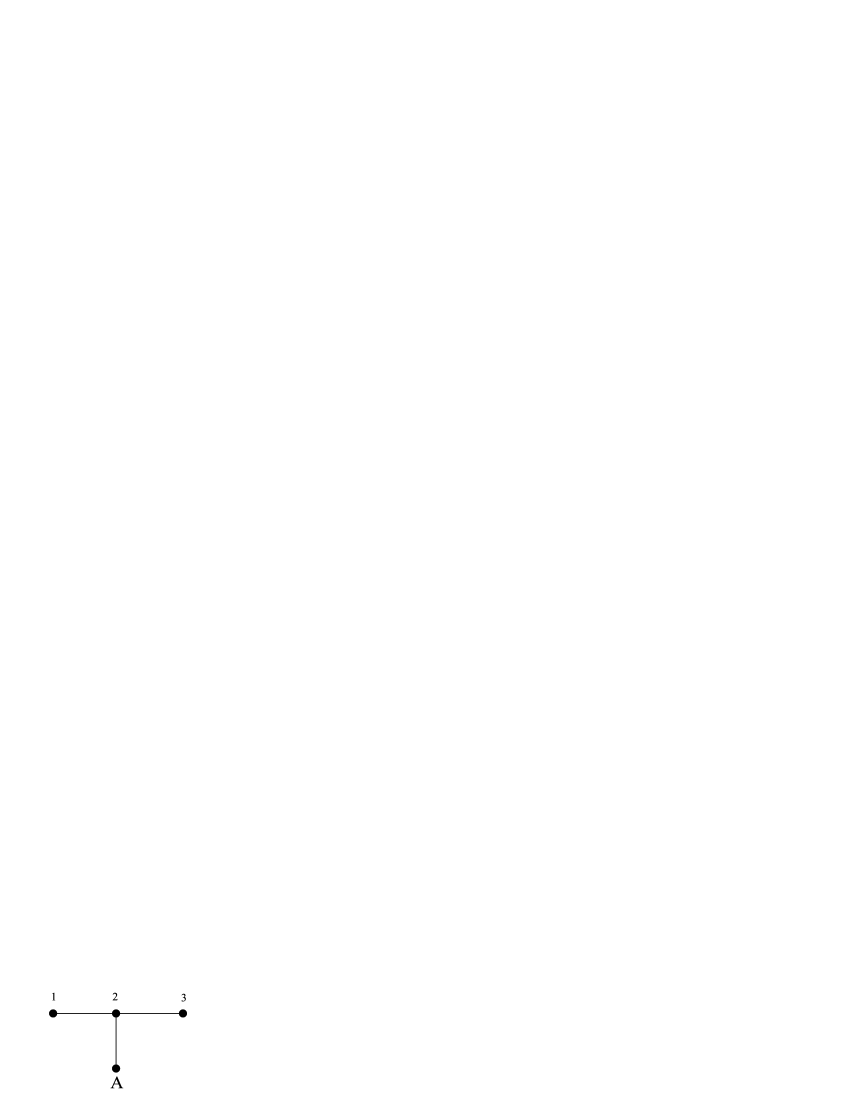
Figure 9: $Z$ measurements are used to eliminate unwanted sites such as A.

Suppose we wish to use only the linearly arranged sites 1,2,3 i.e. we want to delete site A. Consider $Z_{A}$, a $Z$ measurement at site A, with outcome $k_{A}$. To see its effect recall that the pattern in figure 9 is obtained by applying $CZ$ operations to a set of four $\left|+\right\rangle$ states, located at the sites. But measurement $Z_{A}$ commutes with $CZ_{12}$ and $CZ_{23}$ so starting with the four $\left|+\right\rangle$ states we can first do $CZ_{A2}$ and then $Z_{A}$ before $CZ_{12}$ and $CZ_{23}$. But $CZ_{A2}\left|+\right\rangle\left|+\right\rangle=\left|0\right\rangle\left|+\right\rangle+\left|1\right\rangle\left|-\right\rangle$ so after the $Z_{A}$ measurement (with outcome $k_{A}$) the sites 1,2,3 contain $\left|+\right\rangle\left|(-1)^{k_{A}}\right\rangle\left|+\right\rangle$ i.e. the effect of the $Z_{A}$ measurement is to have used the Hadamard basis state $\left|(-1)^{k_{A}}\right\rangle$ at site 2 instead of the standard $\left|+\right\rangle$ (with no site at A) and then entangle as usual. Next consider the basic 1WQC single step of figure 7 with $\left|-\right\rangle$ instead of $\left|+\right\rangle$ at site 2: we start with $\left|\psi\right\rangle\left|-\right\rangle$, apply $CZ$, then do $M(\theta)$ at qubit 1 for output at qubit 2. But this is the same as the following: start with $\left|\psi\right\rangle\left|+\right\rangle$, then (i) apply $CZ$, (ii) do $M(\theta)$ on qubit 1, then (iii) perform the unitary operation $I_{1}\otimes Z_{2}$. This is identical to the previous process because (iii) commutes with (i) and (ii) so we can change the order to (iii), then (i) then (ii) and note that $Z_{2}\left|+\right\rangle=\left|-\right\rangle$. A similar argument applies to each neighbour of A if there is more than one. In summary, we see that a $Z_{A}$ measurement (outcome $k_{A}$) at a site A adds in an extra $Z^{k_{A}}$ Pauli correction at all neighbouring sites of A, in addition to the usual Pauli operations arising from measurement patterns in a standard cluster state that had site A absent from the start.

$Z$ measurements also have a second role: as in TQC they are applied to a final state of a computation to produce the classical output results. So just as in TQC we have the curious feature that these “final” $Z$ measurements are always non-adaptive and can be applied first, before any of the computation itself has been implemented!

To briefly summarise the 1WQC model, we have seen that any quantum gate array can be translated into a pattern of 1-qubit measurements on a suitably large 2-dimensional cluster state. Choices of measurement bases are generally adaptive i.e. possibly depending on previous measurement outcomes. Thus the 1-qubit measurements are organised into layers and the measurements within each layer can be done simultaneously in parallel. The output qubits (always measured in the $Z$ basis) can always be done in the first layer. This temporal sequencing “cuts across” the temporal sequence of the original gate array – all gates are generally done “partially” in each layer and simultaneously built up as the layers accumulate. Just as in TQC, arrays of Clifford operations can always be fully implemented with only one layer of measurements.

6 Further features of 1WQC

6.1 A further parallelisability result

Any polynomial sized quantum gate array can be implemented in 1WQC using at most a polynomial number of measurement layers (c.f. section 8 later). Also we have seen that any array of Clifford operations can be implemented with just one layer of measurements. This suggests the following interesting question: which classes of quantum gate arrays can be implemented in 1WQC with constraints on the number of measurement layers e.g. using 2 or 3 or a logarithmic number of layers? Does the latter include all polynomial time quantum computation? Although very little is known about such questions, we have the following result of Raussendorf and Briegel [6, 12]. Its proof depends on more subtle properties of Pauli propagation relations for particular operations.

Theorem:   Any gate array using gates from the set $\{CX,R_{x}(\theta)\,\,{\rm all}\,\,\theta\}$ or from the set $\{CX,R_{z}(\theta)\,\,{\rm all}\,\,\theta\}$ can be implemented with just two measurement layers.

Remark: Neither of these sets is believed to be universal although it is known that $CX$ with all $y$-rotations is universal [13].

Proof of theorem:   We give a proof for $x$-rotations. (The case of $z$-rotations is similar). We use the following three (easily verified) facts: (i) any single $M(\theta)$ measurement (e.g. as shown in figure 7) generates only $I$ or $X$ Pauli corrections. They may become $Z$’s only after propagation through other gates. (ii) when Pauli operations are commuted across the Clifford operation $CX$, $X$ propagates only to $X$’s (and $Z$ propagates only to $Z$’s) although the Pauli operator may spread from one qubit onto two qubits. (iii) The $R_{x}$ gate may be implemented in 1WQC using the measurement pattern shown in figure 10.

Figure 10: The process above leaves qubit 3 in state $X^{s_{2}}Z^{s_{1}}R_{x}((-1)^{s_{1}}\theta)\left|\psi\right\rangle$. Thus to implement a given $x$ rotation the sign of the angle $\theta$ is adaptive, depending on the measurement outcome $s_{1}$.

Now consider any gate array $\ldots G_{3}G_{2}G_{1}$ where each $G_{i}$ is a $CX$ or an $x$-rotation gate. Set up its corresponding measurement pattern (using figure 10 for each $x$-rotation gate). $CX$ is a Clifford operation and involves no adaptive measurements. In the first measurement layer we perform all $CX$ pattern measurements and all $X$ measurements of the $R_{x}$ gates (i.e. all qubit 1 measurements in figure 10). This produces some extraneous Pauli operations and leaves only the $M(-\theta)$ nodes unmeasured (i.e. all qubit 2’s in figure 10). Next commute all these Pauli’s out to the left hand end of the gate array. This commutation leaves all $CX$’s unchanged (as $CX$ is Clifford) but some $x$-rotation angles acquire an unwanted minus sign (c.f. propagation relations for $x$-rotations given previously). Thus reset these altered angle signs so that the $M(-\theta)$ measurements again give the correct designated gates i.e. make the adaptive choice of bases for the next measurement layer. Finally in the second layer, perform all the $M(-\theta)$ measurements. We again get some further extraneous Pauli operations generated. By (i) we get only $I$ or $X$, but these can be harmlessly commuted out to the left since $X$ commutes with $x$-rotations and $CX$ preserves $X$’s in its propagation relations (i.e. no $Z$’s are generated). $\Box$

6.2 Non-universality of one-dimensional clusters

We have seen that 1WQC with two-dimensional cluster states is universal for quantum computation. Nielsen and Doherty [14] have shown that any 1WQC process based on only 1-dimensional cluster states can be simulated classically efficiently i.e. in polynomial time in the number of qubits. Thus the universality of any such model would imply that quantum computation is no more powerful than classical computation.

The argument may be paraphrased as follows (ignoring technical issues of precision of the simulation). Consider any state of the form shown in figure 11.

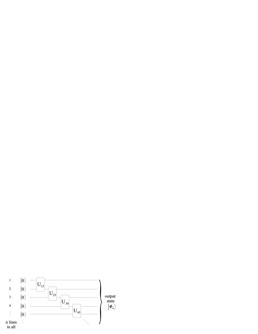
Figure 11: A generalised 1-dimensional cluster state $\left|\Phi_{n}\right\rangle$. Starting with a row of $n$ qubits each in state $\left|0\right\rangle$ we sequentially apply $U_{i,i+1}$ to qubits $i,i+1$ as shown in the above gate array having a ladder-like structure.

(The standard cluster state is obtained by choosing each $U_{i,i+1}$ to be $CZ(H\otimes H)$). Consider now any sequence of 1-qubit measurements such that for later measurements, the choice of measurement basis and even the choice of qubit used, may both depend on outcomes of earlier measurements. Then the whole process may be classically simulated in polynomial (in $n$) time i.e. the resulting probability distribution of outcomes may be sampled by classical means in polynomial time.

The proof runs as follows. At a general stage suppose measurements on lines $a,b,\ldots,p,q$ have already been simulated and the chosen sample outcomes are $a^{\prime},b^{\prime},\ldots,p^{\prime},q^{\prime}$ respectively. Even though these measurements may have been chosen adaptively, once the outcomes have been specified (as $a^{\prime},b^{\prime},\ldots,p^{\prime},q^{\prime}$) we can perform the measurements in any order we wish to compute the joint probability $P(a^{\prime},b^{\prime},\ldots,p^{\prime},q^{\prime})$ of the designated outcome string. Now suppose the next measurement is on line $k$. To sample its outcome distribution we need to know

$$P(k^{\prime}|a^{\prime},b^{\prime},\ldots,p^{\prime},q^{\prime})=\frac{P(a^{\prime},b^{\prime},\ldots,k^{\prime},\ldots,p^{\prime},q^{\prime})}{P(a^{\prime},b^{\prime},\ldots,p^{\prime},q^{\prime})}.$$

Here $a^{\prime},b^{\prime},\ldots,p^{\prime},q^{\prime}$ have their fixed values and we take $k^{\prime}=0,1$ separately. Having computed this probability we sample $k^{\prime}$ to give a definite value, and continue in the same way for the next measurement on some line, $l$ say.

To show that this whole process is efficient, we need only show that $P(a^{\prime},b^{\prime},\ldots,p^{\prime},q^{\prime})$ can be computed in poly$(n)$ time for any chosen set of values $a^{\prime},b^{\prime},\ldots,p^{\prime},q^{\prime}$, on any chosen set of lines. Without loss of generality suppose these lines are listed in increasing order of occurrence from line 1 at the top. Note that we can regard a measurement on any line, $a$ say, as occurring immediately after $U_{a,a+1}$ and before $U_{a+1,a+2}$. Let $\rho_{m}$ denote the reduced state of any line $m$ at the position in between the application of $U_{m-1,m}$ and $U_{m,m+1}$, and let $\sigma_{m,m+1}$ denote the application of $U_{m,m+1}$ to $\rho_{m}\otimes\left|0\right\rangle\left\langle 0\right|$.

Starting at the top we compute $\sigma_{12}$ as $U_{12}$ on $\left|0\right\rangle\left|0\right\rangle$. Then compute $\rho_{2}$ by partial trace, tracing out system 1 from $\sigma_{12}$. Then compute $\sigma_{23}$ as $U_{23}$ on $\rho_{2}\otimes\left|0\right\rangle\left\langle 0\right|$ etc. continuing until $\sigma_{a,a+1}$ where the first measurement occurs. At this point we do not compute $\rho_{a+1}$ as the partial trace above but instead, apply to $\sigma_{a,a+1}$ the projector corresponding to measurement outcome $a^{\prime}$, obtaining a subnormalised state $\rho_{a+1}$ on line $a+1$. In fact $\mbox{Tr}\,\rho_{a+1}$ is the probability of getting outcome $a^{\prime}$ in the $a$-line measurement. We continue in this way computing the reduced states of the lines successively (using the measurement projector at any measured line and partial trace at any unmeasured line) until we have applied the last ($q^{\prime}$) measurement projector. The trace of this final resulting state is then $P(a^{\prime},b^{\prime},\ldots,p^{\prime},q^{\prime})$. At each stage of this calculation we need to hold the state of at most two lines (i.e. not $n$ lines with its exponentially large description) and we pass through the ladder $n$ times, once for each successive measurement. Hence the whole calculation is completed in time polynomial in $n$. This feature of the calculation is a consequence of the special ladder-like structure of figure 11 and it does not apply to general gate arrays.

7 Relationships between the TQC and 1WQC models

The two models have several similarities – both are based on measurements as computational steps and both have the awkward feature of supplementing desired gates with unwanted Pauli operations. But there are also some essential differences: TQC uses (Bell) measurements on 2 or more qubits whereas 1WQC uses only 1-qubit measurements. 1WQC starts with a cluster state having multi-partite entanglement across all the qubits whereas TQC is based on a state comprising only bipartite entangled pairs.

The models can be related in several different ways. We will discuss three of them. The relationships serve to improve our understanding of 1WQC and its measurement patterns. For TQC the relation between the measurement and the desired gate is already transparent.

Our first way of relating TQC and 1WQC was proposed by Aliferis and Leung[15]. The basic idea is to identify suitable pairs of consecutive 1-qubit measurements in 1WQC with a Bell measurement of a teleportation. This approach is strongly suggested by patterns such as the one in figure 6. With reference to the basic teleportation scheme in figure 1 we note the following. $CX$ transforms Bell states into product states:

$$CX\left|B_{ij}\right\rangle=\left|(-1)^{j}\right\rangle\left|i\right\rangle$$

(where the first ket is a $\left|\pm\right\rangle$ state according to the given sign). Hence the Bell measurement on 12 can be performed by the entangling operation $CX$ followed by the 1-qubit measurements $X_{1}$ and $Z_{2}$. Similarly the $\left|B_{00}\right\rangle$ state of 23 is $CX\left|+\right\rangle_{2}\left|0\right\rangle_{3}$ which we can alternatively write as $CX\left|+\right\rangle_{3}\left|0\right\rangle_{2}$ (where subscripts denote the qubit number and we adopt the notation for the asymmetrical $CX$ operation that the first qubit listed is the control qubit). Thus teleportation fully decomposes into entangling operations and 1-qubit measurements as shown in figure 12.

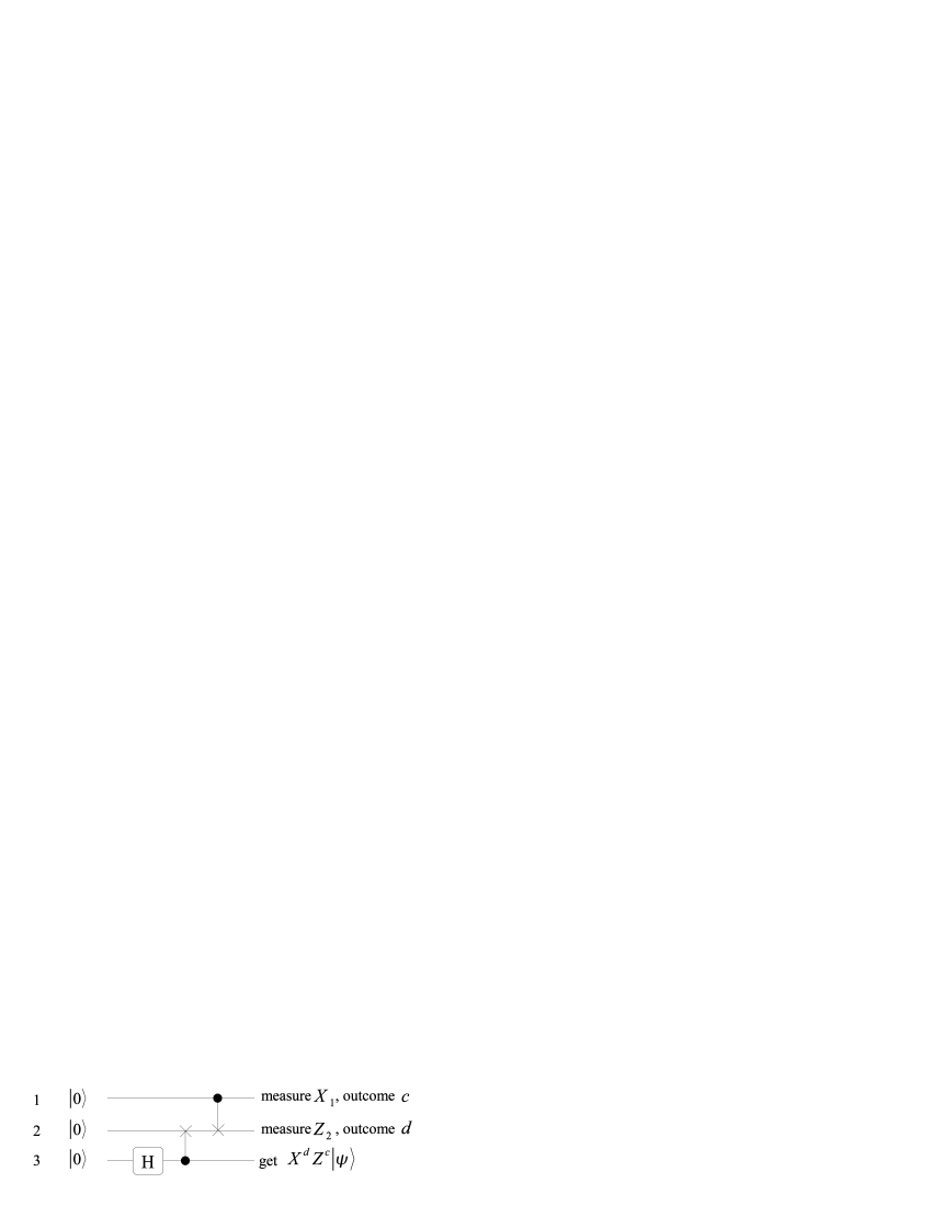
Figure 12: Teleportation as entangling operations and 1-qubit measurements. The diagram is read from left to right. The vertical lines denote $CX$ operations with control and target marked as $\bullet$ and X respectively. Note that the two $CX$ operations, with the shown opposite orientations, commute. Alternatively we could have put $H$ on line 2 and the first $CX$ the other way up, but then the two $CX$’s would not commute.

So, in view of figure 12 teleportation can be interpreted as: start with $\left|\psi\right\rangle_{1}\left|0\right\rangle_{2}\left|+\right\rangle_{3}$, entangle suitably with $CX$’s, then do $X_{1}$ and $Z_{2}$ measurements, which is structurally just like the 1WQC paradigm. But we have a slight mismatch in choice of primitives: TQC uses $CX$ and $\left|B_{00}\right\rangle$ states whereas 1WQC is based on $CZ$ and $\left|H\right\rangle=CZ\left|+\right\rangle\left|+\right\rangle$ states, so the correspondence involves a sprinkling of Hadamard operations to interconvert these ingredients.

Extending this idea, we find that other pairs of of measurements in 1WQC (such as $X_{1}M(\theta)_{2}$ and $M_{1}(\theta)X_{2}$) can be interpreted as rotated Bell measurements, but only special pairs of such consecutive 1-qubit measurements can be fused together to form Bell measurements. We refer to [15] for further details that we will not need here. Although we are able to reconstruct rotated Bell measurements for the 1WQC implementation of a full universal set of gates, this interpretation of 1WQC has the drawback that single 1-qubit measurements individually cannot be interpreted in terms of TQC.

Our second relationship between TQC and 1WQC, proposed by Childs et al.[16] and Jorrand et al.[17], is a further development of the ideas in figure 12. As noted in the caption, the two $CX$ operations commute. Also the $X_{1}$ measurement commutes with all subsequent operations on 23. Thus we can change the order of actions to: (entangle 12, measure $X_{1}$), then (entangle 23, measure $Z_{2}$), obtaining a sequence of two operations of the same form viz. (entangle 12, measure 1) to obtain a state at 2. As noted in figure 7, it is exactly this kind of operation that drives 1WQC too, so we can regard it as a common fundamental primitive underlying both models (and sometimes called “one-bit teleportation”).

A slight awkwardness in figure 12 is the lack of uniformity of actions: the $CX$’s act in opposite orientations (necessary for commutativity) and we have a single $H$ gate as well. But this can be easily remedied: instead of the usual Bell state based teleportation scheme we consider teleportation with maximally entangled state $\left|H\right\rangle=CZ\left|+\right\rangle\left|+\right\rangle$ at 23 and its associated Bell measurement on 12 given by the basis

$$\{I\otimes I\left|H\right\rangle,X\otimes I\left|H\right\rangle,Z\otimes I\left|H\right\rangle,XZ\otimes I\left|H\right\rangle\}.$$ (3)

Then note that $CZ$ maps this basis to $\{\left|+\right\rangle\left|+\right\rangle,\left|+\right\rangle\left|-\right\rangle,\left|-\right\rangle\left|-\right\rangle,\left|-\right\rangle\left|+\right\rangle\}$ so the Bell measurement is equivalent to applying $CZ$ and then measuring $X_{1}$ and $X_{2}$. Also unlike $CX$, $CZ$ is symmetrical so the picture as in figure 12 for this teleportation process is fully uniform. The two “one-bit teleportations” are now identical, in fact corresponding exactly to the process in figure 6, implemented sequentially.

7.1 Matrix product state relationship of TQC and 1WQC

Our third and most remarkable connection between TQC and 1WQC, proposed by Verstraete and Cirac[18], is based on the formalism of so-called valence bond solids or matrix product states. In this correspondence each single 1-qubit measurement of 1WQC will be interpreted in terms of a full single teleportation.

Consider a 2-dimensional grid of states $\left|H\right\rangle=CZ\left|+\right\rangle\left|+\right\rangle$ as shown in figure 13. Let $\left|\rm grid\right\rangle$ denote the total state of all the qubits.

Figure 13: Valence bond solid or matrix product state for the cluster state. Each “valence bond” line denotes the maximally entangled state $\left|H\right\rangle$ of two qubits. Each site (circled) has 4 or 3 or 2 qubits. At each site we consider the two dimensional subspace spanned by the two kets of “all zeroes” and “all ones”.

At each site in the figure consider the two dimensional subspace spanned by $\{\left|00\ldots 0\right\rangle,\left|11\ldots 1\right\rangle\}$ and the associated projector, renaming these two basis states as $\left|\tilde{0}\right\rangle$ and $\left|\tilde{1}\right\rangle$:

$$\Pi=\left|\tilde{0}\right\rangle\left\langle 00\ldots 0\right|+\left|\tilde{1}\right\rangle\left\langle 11\ldots 1\right|.$$

Applying $\Pi$ to $\left|\rm grid\right\rangle$ we obtain a state with a single qubit at each site (and subnormalised because of the projection).

Lemma 3:   The multi-qubit state $\Pi\left|\rm grid\right\rangle$ (after normalisation) is precisely the 1WQC cluster state.

Proof:   We first note the fact of figure 14.

Figure 14: Dots denote qubits and the connecting line denotes the maximally entangled state $\left|H\right\rangle$. If we project each circled site to span$\{\left|00\right\rangle,\left|11\right\rangle\}$ then the resulting state (after normalisation) is $CZ\left|\psi_{1}\right\rangle\left|\psi_{2}\right\rangle$.

Now consider a 1-dimensional grid of $\left|H\right\rangle$ states as in figure 15.

Figure 15: One dimensional valence bond solid.

Apply $\Pi$ at each node. Each bond is already $CZ\left|+\right\rangle\left|+\right\rangle$ by definition. By the fact in figure 14 the projections at sites 23 and 45 simply serve to apply $CZ$ between qubits 2 and 5. Hence the whole projected state is just $CZ$ applied to all connecting pairs in $\left|+\right\rangle\left|+\right\rangle\ldots\left|+\right\rangle$ i.e. the 1-dimensional cluster state. This argument easily generalises to the 2-dimensional geometry of figure 13.$\Box$

Next consider using $\left|H\right\rangle$ states for TQC via application of rotated versions of the associated basic Bell measurement eq. (3). For clarity of the essential idea, consider the 1-dimensional case of figure 15. Let us calculate the rotated Bell basis corresponding to the 1-qubit gate

$$W(-\theta)=\frac{1}{\sqrt{2}}\left(\begin{array}[]{cc}1&e^{-i\theta}\\ 1&-e^{-i\theta}\end{array}\right).$$

The basis is given by

$$\left|a\right\rangle=(W(-\theta)^{\dagger}\sigma_{a})\otimes I\left|H\right\rangle$$

where $a=0,1,2,3$ and $\sigma_{0}=I$, $\sigma_{1}=X$, $\sigma_{2}=Z$, $\sigma_{3}=XZ$. A direct calculation gives the first two states as

$$\begin{array}[]{c}\left|a=0\right\rangle=\frac{1}{\sqrt{2}}(\left|00\right\rangle+e^{i\theta}\left|11\right\rangle)\\ \left|a=1\right\rangle=\frac{1}{\sqrt{2}}(\left|00\right\rangle-e^{i\theta}\left|11\right\rangle)\end{array}$$

and the remaining two span the orthogonal complement of span$\{\left|00\right\rangle,\left|11\right\rangle\}$ at the site. Thus remarkably these first two Bell states lie within the 1-qubit subspace determined by the $\Pi$-projection. Furthermore this part of the Bell measurement corresponds precisely to the measurement basis $M(\theta)=\{\left|\tilde{0}\right\rangle\pm e^{i\theta}\left|\tilde{1}\right\rangle\}$ on the projected site i.e. on the cluster state. (Note that for other more general 1-qubit gates $U$, the corresponding rotated Bell basis states do not generally lie in a simple way relative to the $\Pi$-projected subspaces.)

Stated otherwise, $M(\theta)$ measurements on the cluster state (which is the basic ingredient of 1WQC, c.f. figure 7) can be thought of as teleportations in the TQC formalism, where the teleportations always produce one of the $a=0,1$ outcomes (and not $a=2,3$) i.e. teleportations that have been “cut down” by the $\Pi$ projection. In a similar way all other 1WQC ingredients (viz. $Z$ measurements and the $CZ$ measurement pattern) can be seen as descendants under the $\Pi$ projection of teleportations on a valence bond grid state $\left|\rm grid\right\rangle$. We omit further details which may be found in [18].

8 Measurement based models and computational complexity

The gate array model of quantum computation provides a transparent formalism for the theoretical study of quantum computation and its computational complexity features compared to classical computation. So why should we bother with further exotic models such as the measurement based models? Indeed our measurement based models are readily seen to be polynomial time equivalent to the gate array model i.e. each model can simulate the other with only a polynomial (i.e. modest) overhead of resources (number of qubits and computational steps). To see this first recall that the standard gate array model (allowing measurements only at the end and only in the $Z$ basis) can be easily generalised to allow measurements along the way with subsequent choices of further gates and measurements being allowed to depend on earlier measurement outcomes. Indeed consider a measurement in a basis $\{U\left|0\right\rangle,U\left|1\right\rangle\}$ on a qubit B applied during the course of a gate array process. To regain the standard gate array paradigm, for each such measurement we adjoin an extra ancillary qubit A, initially in state $\left|0\right\rangle$ and replace the measurement by the following: apply $U^{\dagger}$ to B and the apply $CX$ to qubits BA. This simulates a coherent representation of the measurement in which qubit A plays the role of a pointer system. Subsequent gates that depend on the measurement outcome are replaced by a corresponding controlled operation, controlled by the state of A (written in the $Z$ basis). In this way we purge all intermediate measurements from the body of the array and a measurement of each ancilla in the $Z$ basis at the end results in a standard gate array process which is equivalent to the given non-standard one.

Using the above technique any 1WQC process is easily converted into an equivalent (standard) gate array process. We first build the required cluster state using an array of $CZ$ gates acting on $\left|+\right\rangle=H\left|0\right\rangle$ states and introduce an ancilla A for each 1-qubit 1WQC measurement. For each $M(\theta)$ measurement we introduce an extra gate $W^{\dagger}(\theta)$ which transforms the $M(\theta)$ basis to the standard basis. The overhead in number of qubits and gates in this simulation is at most linear.

Conversely given any gate array (based say on one of our previously considered universal sets of gates) we have seen how it can be translated into a measurement pattern on a suitably large cluster state. If $K$ is the largest size of the 1WQC measurement pattern for any gate in our universal set then the number of qubits and computational steps increases by at most a factor of $K$ i.e. the resource overhead is again linear.

Polynomial time equivalence of computational models is important in computational complexity theory because such models have the same class of polynomial time computations. But polynomial time equivalence does not preserve more subtle structural features of computations, such as parallelisability. Indeed already in the context of classical computation it is well known that the (one tape) turing machine model is polynomial time equivalent to the (classical) gate array model yet the turing machine model does not even have a natural notion of parallalisability at all, whereas the gate array model does! (i.e. doing gates simultaneously in parallel).

In contrast to the quantum gate array model, the formalism of measurement based models offers new perspectives for parallelisability issues. We have already noted the fundamental feature that measurements on different subsystems of an entangled state always commute so long as the choice of measurement is not adaptive i.e. not dependent on the outcome of another measurement. We have seen examples of processes which are inherently sequential for gate arrays (e.g. sequences of Clifford gates) that become parallelisable in the measurement based models.

The measurement based models have a further novel feature: they provide a natural formalism for separating a quantum algorithm into “classical parts and quantum parts”. In contrast, in the gate array model every computational step is viewed as being quantum. The notion of classical-quantum separation becomes more compelling when we consider say, Shor’s algorithm in its full totality, including the significant amount of non-trivial classical post-processing of measurement results needed to reach the final answer. It seems inappropriate to view this post-processing as a quantum process (albeit one that maintains the computational basis)!

In measurement based computation the quantum parts of the algorithm are the quantum measurements done in parallel layers and the interspersed classical parts correspond to the adaptive choices of measurement bases, determined by classical computations on the previous layers’ measurement outcomes. We may generalise this formalism in the following way: we allow (adaptively chosen) unitary gates as well as measurements within the quantum parts. We allow quantum layers to have only depth 1 (so a depth $K$ quantum process is regarded as $K$ layers with no interspersed classical computations) whereas classical layers can have any depth i.e. we are less concerned about controlling their structure.

In this formalism any quantum computation is viewed as a sequence of classical and quantum layers. The total quantum state is passed from one quantum layer to the next and the quantum actions carried out in the next layer are determined by classical computations on measurement outcomes from previous layers.

Any polynomial time quantum computation (say in the gate array model) can clearly be implemented with a polynomial number of quantum layers (and no interspersed classical layers) but the above formalism suggests a novel structural conjecture:

Conjecture:    Any polynomial time quantum algorithm can be implemented with only $O(\log n)$ quantum layers interspersed with polynomial time classical computations. $\Box$

This conjecture, asserting an exponential reduction in the essential “quantum content” of any quantum algorithm, has no analogue in classical complexity theory (where there is no notion of classical-quantum separation). Intuitively we are conjecturing that polynomial time classical computation needs relatively little “quantum assistance” to achieve the full power of polynomial time quantum computation. Although the conjecture remains unproven in general, we note that Cleve and Watrous [19] have shown that it holds true for Shor’s algorithm.

9 Acknowledgements

These notes were developed in the course of presentations of the subject matter at a series of summer schools and workshops: the CNRS summer school on quantum logic and communication, Corsica, August 2004, the workshop on quantum information and computation, Newton Institute, Cambridge UK, August – December 2004, the NATO-ASI summer school on quantum computation and quantum information, Crete, May 2005 and the JST summer school on quantum information, Kochi, Japan, August 2005. Thanks to Sean Clark and Noah Linden for discussions of the material and to Sean Clark for providing the figures. This work was partially supported by the EU project RESQ-IST-2001-37559 and the UK EPSRC Interdisciplinary Research Collaboration on Quantum Information Processing.

References

- [1] C. Bennett, G. Brassard, C. Crepeau, R. Jozsa, A. Peres and W. Wootters, Teleporting an unknown quantum state via dual classical and Einstein-Podolsky-Rosen channels, Phys. Rev Lett. 70, 1895-1899, 1993.
- [2] D. Gottesman and I. Chuang, Quantum teleportation as a universal computational primitive, Nature 402, 390-393, 1999. arXiv:quant-ph/9908010.
- [3] M. A. Nielsen. Quantum computation by measurement and quantum memory. Phys. Lett. A, 308, 96–100, 2003. arXiv:quant-ph/0108020.
- [4] D. W. Leung. Quantum computation by measurements, Int. J. Quant. Inf. 2, 33-43, (2004) arXiv:quant-ph/0310189, 2003. D. W. Leung. Two qubit projective measurements are universal for quantum computation. arXiv:quant-ph/0111122, 2001.
- [5] R. Raussendorf and H. J. Briegel, A one-way quantum computer. Phys. Rev. Lett., 86, 5188–5191, 2001. arXiv:quant-ph/0010033.
- [6] R. Raussendorf, D. E. Browne, and H. J. Briegel. Measurement-based quantum computation with cluster states Phys. Rev. A, 68, 022312, 2003. arXiv:quant-ph/0301052.
- [7] M. A. Nielsen and C. M. Dawson. Fault-tolerant quantum computation with cluster states. arXiv:quant-ph/0405134, 2004.
- [8] R. F. Werner, All teleportation and dense coding schemes, arXiv:quant-ph/0003070, 2000.
- [9] D. Gottesman, Stabilizer Codes and Quantum Error Correction, PhD thesis, California Institute of Technology, Pasadena, CA, 1997. arXiv:quant-ph/9705052. See also D. Gottesman, Course on quantum error correction, Perimeter Institute, Waterloo http://perimeterinstitute.ca/people/researchers/dgottesman/CO639-2004/index.html
- [10] M. A. Nielsen and I. Chuang, Quantum Computation and Information, CUP 2000, page 464.
- [11] S. Aaronson and D. Gottesman, Improved simulation of stabiliser circuits. arXiv:quant-ph/0406196, 2004.
- [12] R. Raussendorf and H. J.Briegel, Computational model underlying the one-way quantum computer. Quant. Inf. Comp. 2, 433, 2002. arXiv:quant-ph/0108067, 2001.
- [13] Yaoyun Shi, Both Toffoli and Controlled-NOT need little help to do universal quantum computation. arXiv:quant-ph/0205115, 2002.
- [14] M. A. Nielsen, Cluster-state quantum computation, to appear in Rev. Math. Phys. arXiv:quant-ph/0504097, 2005.
- [15] P. Aliferis and D. W. Leung, Computation by measurements: a unifying picture. arXiv:quant-ph/0404082, 2004.
- [16] A. M. Childs, D. W. Leung, and M. A. Nielsen, Unified derivation of measurement-based schemes for quantum computation. arXiv:quant-ph/0404132, 2004.
- [17] P. Jorrand and S. Perdrix, Unifying quantum computation with projective measurements only and one-way quantum computation. arXiv:quant-ph/0404125, 2004.
- [18] F. Verstraete and J. I. Cirac, Valence bond solids for quantum computation. Phys. Rev. A, 70, 060302 (R), 2004. arXiv:quant-ph/0311130.
- [19] R. Cleve and J. Watrous, fast parallel circuits for the quantum Fourier transform, Proceedings of the 41st Annual IEEE Symposium on Foundations of Computer Science (FOCS 2000), 526-536, 2000. arXiv:quant-ph/0006004, 2000.