Rapid State-Reduction of Quantum Systems Using Feedback Control

Abstract

We consider using Hamiltonian feedback control to increase the speed at which a continuous measurement purifies (reduces) the state of a quantum system, and thus to increase the speed of the preparation of pure states. For a measurement of an observable with $N$ equispaced eigenvalues, we show that there exists a feedback algorithm which will speed up the rate of state-reduction by at least a factor of $2(N+1)/3$.

To perform information processing using quantum systems the systems in question must be prepared in pure states QCreview . Due to environmental noise such systems often exist naturally in mixed states, and either a process of cooling Tannor or measurement must be used to purify them. While it is often assumed for the sake of simplicity that measurements are instantaneous, this is not the case in reality. All physical processes happen on some finite time scale, and measurement is no exception. Thus every von Neumann measurement is in fact a continuous measurement which has been run for sufficiently long. The speed at which one can measure a system will therefore place limits on the speed at which measurement can be used as a tool to prepare initial states.

Given a fixed measurement rate, it is possible to use Hamiltonian feedback B88 ; YK98 ; WM93b ; DJ99 ; DHJMT00 ; MJ04 during the measurement to increase the speed at which the system is purified. For a single qubit this problem was analyzed by Jacobs J03 . For this case the optimal feedback algorithm will produce a factor of 2 increase in the speed at which a given level of purity can be obtained. This speed-up factor is achieved in the limit in which the desired purity is high, being the limit in which the measurement time is large compared to the measurement rate. Shorter measurement times result in a smaller speed-up. The speed-up is a quantum mechanical effect, in that the equivalent measurement on a classical bit cannot be enhanced in this manner; for a two-state system a speed-up is only possible if the system can exist in a superposition of the eigenstates of the measured observable during the process. Specifically, the optimal algorithm consists of measuring $\sigma_{z}$, and using Hamiltonian feedback to continually rotate the state of the system as needed so that it remains diagonal in the $\sigma_{x}$ basis throughout the measurement. This requires a process of real-time feedback, since the required stream of unitary operations depends upon the continuous stream of measurement results.

Here we consider using feedback to enhance a measurement on a system of arbitrary size. This problem is considerably more complex than that of a single qubit, because one cannot directly derive the analytical results which are available in that case FJ01 . We will consider a continuous measurement of an observable with $N$ distinct, equally spaced eigenvalues (i.e. one that distinguishes the $N$-states), present a feedback algorithm, and prove a lower bound on its performance. Using this lower bound we show that the speed-up factor which the algorithm provides in the long time limit is at least $2(N+1)/3$. Thus for large systems Hamiltonian feedback can greatly enhance the rate of state-reduction.

The evolution of a system under the continuous measurement of an observable $X$ is given by measnote ; Bxx ; K00 ; C93 ; WM93 ; BS88 ; D86 ; B87

$$d\rho=-\gamma[X,[X,\rho]]dt+\sqrt{2\gamma}(X\rho+\rho X-2\langle X\rangle\rho)dW,$$ (1)

where $\rho$ is the density matrix of the system and $dW$ is an increment of the Wiener process, describing driving by Gaussian white noise, and $\gamma$ is a positive constant often referred to as the measurement strength. The continuous stream of measurement results, $y(t)$, is given by $dy(t)=\langle X(t)\rangle dt+dW/\sqrt{8\gamma}$. The effect of such a measurement in the long time limit is to project the system onto one of the eigenstates of $X$, producing a von Neumann measurement in the basis of $X$.

The rate at which the measurement distinguishes between two eigenstates of $X$ is proportional to $\gamma$ multiplied by the difference between the respective eigenvalues. In order to able to purify any initial state the observable must therefore possess non-degenerate eigenvalues. As mentioned above we will also assume that the eigenvalues of $X$ are equally spaced. This is true, for example, if the system has total angular momentum $j$, and the observable is the $z$-component of angular momentum, $J_{z}$. In this case there are $N=2j+1$ states, with eigenvalues $-j,\ldots,j$. Further, since Eq.(1) is invariant under the transformation $X\rightarrow X^{\prime}=X+\alpha I$ for any real $\alpha$, an overall shift in the eigenvalues of the measured observable has no effect on the measurement. As a result, without loss of generality we may always assume that $X$ is traceless. Under the restriction that the eigenvalues are equally spaced, we may therefore always assume that $X$ is proportional to $J_{z}$, where $j=(N-1)/2$. While the constant of proportionality is unimportant for the purposes of our analysis, we will define $X$ so that its eigenvalues are separated by $1/N$. Thus $X=J_{z}/N$.

Using the algorithm in J03 as a guide, we will consider a feedback algorithm consisting of a measurement of $X$, in which the feedback is used to rotate the state of the system so that the eigenbasis of the density matrix remains unbiased with respect to the eigenbasis of $X$ during the measurement. Recall that two bases are unbiased with respect to one another when the moduli of the elements of the matrix which transforms between them are all identical Wxx . We will refer to the eigenbasis of $X$ as the measurement basis. To implement such an algorithm one applies a Hamiltonian in each time interval to rotate the state of the system so as to cancel the infinitesimal change in the eigenbasis caused by the measurement in that time interval. In analyzing the performance of this algorithm, we will use the impurity, $L=1-\mbox{Tr}[\rho^{2}]$ Lnote , as a our measure of mixedness, rather than the von Neumann entropy, because it has a very simple analytical form. In addition, the impurity is equal to the von Neumann entropy in the limit of high purity.

To begin with we calculate the instantaneous derivative of $L$ when the measurement basis is unbiased with respect to $\rho$. In this case, if we work in the eigenbasis of $\rho$, all the diagonal elements of $X$ are the same, and equal to $\langle X\rangle$, and we have further that $\mbox{Tr}[X^{n}\rho^{m}]=\langle X^{n}\rangle\mbox{Tr}[\rho^{m}]$. Using this fact in Eq.(1) we find that the evolution of $L$ is particularly simple:

$$dL=-8\gamma Tr[X\rho X\rho]dt.$$ (2)

That is, when the measurement basis is unbiased with respect to $\rho$, the evolution of the impurity over the succeeding infinitesimal time step is deterministic. In the absence of any feedback, the action of the measurement changes the eigenbasis of $\rho$, so that the measurement does not remain unbiased. Under our feedback algorithm, however, Eq.(2) remains true, and the purity therefore evolves deterministically.

The key to obtaining a lower bound on the performance of our feedback algorithm is the following lemma.

Lemma 1.

Consider a traceless observable $X$ of an $N$ dimensional quantum system, whose eigenbasis is unbiased with respect to a density operator $\rho$, and consider the $N!$ unitary operators whose action is to permute the eigenvectors of $\rho$. There exists a set of $N!$ operators $X^{(m)}=U_{m}XU_{m}^{\dagger}$ all unbiased with respect to the state $\rho$ of a system, such that when these operators are measured simultaneously with strength $\gamma$, the instantaneous derivative of $L\equiv 1-\mbox{Tr}[\rho^{2}]$ is given by $dL/dt=-8k\gamma N!L$, where $k=\mbox{Tr}[X^{2}]/(N(N-1))$.

Proof.

Consider a simultaneous measurement of $M$ traceless operators $X^{(m)}$ unbiased with respect to $\rho$. From Eq.(2), the derivative of the impurity is

$$dL = -8\gamma dt\sum_{m}Tr[X^{(m)}\rho X^{(m)}\rho]$$ (3)

$$= -8\gamma dt\sum_{m}\sum_{ij}|X_{ij}^{(m)}|^{2}\lambda_{i}\lambda_{j},$$ (4)

where the $X_{ij}^{(m)}$ are the matrix elements of the $X^{(m)}$ in the eigenbasis of $\rho$, and the $\lambda_{i}$ are the eigenvalues of $\rho$. Since the $X^{(m)}$ are traceless, $X_{ii}^{(m)}=0,\;\forall i,m$. Now consider that the $X^{(m)}$ are the $N!$ permutations of a single unbiased traceless operator $X$. In this case, for $i\not=j$ we have $\sum_{m}|X_{ij}^{(m)}|^{2}=(N-2)!\sum_{k}\sum_{l\not=k}|X_{kl}|^{2}=(N-2)!\sum_{kl}|X_{kl}|^{2}\equiv c$. Naturally when $i=j$ we have $\sum_{m}|X_{ij}^{(m)}|^{2}=0$. As a result

$$dL = -8\gamma dt\sum_{ij}c(1-\delta_{ij})\lambda_{i}\lambda_{j}$$ (5)

$$= -8\gamma cdtL.$$ (6)

Permuting the elements of the operator $X$ when written in the eigenbasis of $\rho$ corresponds to a basis change which involves permuting the vectors of the eigenbasis of $\rho$. Such a transformation leaves $X$ unbiased with respect to $\rho$, and thus all the $N!$ operators $X^{(m)}$ are unbiased with respect to $\rho$, and related to $X$ by unitary transformations.

One can also calculate the constant $c$ by using $\sum_{m}Tr[X^{(m)}\rho X^{(m)}\rho]=cdtL$ and setting $\rho=I/N$. The result is $c=(N-2)!\mbox{Tr}[X^{2}]$. ∎

This result shows us two things. The first is that if we measure simultaneously $N!$ unbiased rotated versions of $X$, and combine this with a feedback algorithm which maintains the eigenvectors of $\rho$, the impurity will decay as

$$L(t)=e^{-8\gamma(N-2)!\mbox{\scriptsize Tr}[X^{2}]t}L(0).$$ (7)

The second is that, because we know that the derivative of the impurity when summed over all of the $N!$ measurements is $-8\gamma N!kL$, we know that there is at least one term in this sum for which the derivative is greater than or equal to $-8\gamma kL$. That is, given an unbiased operator $X$, and a density matrix $\rho$, we can always find a transformation $T$ (which permutes the eigenbasis of $\rho$), such that measuring $TXT^{T}$ will provide an instantaneous change in the impurity greater than or equal to $-8\gamma kL$. Of course, we can equivalently apply the transformation to $\rho$, rather than to $X$, which simply involves permuting the eigenvalues of $\rho$.

We can now return to our feedback algorithm. Recall that this involves measuring a single unbiased operator $X$, and applying a unitary operation to the system at each time step to keep the eigenvectors of $\rho$ unchanged. However, using our unitary operation we can also permute the eigenvectors of $\rho$. Therefore, at each time step, we can choose the permutation $T$ so as to maximize the derivative of the impurity. As we have now shown that this maximum derivative is bounded from below by $-8\gamma kL$, we see that our feedback algorithm will produce an impurity $L_{\mbox{\scriptsize fb}}(t)$ such that

$$L_{\mbox{\scriptsize fb}}(t)\leq e^{-8\gamma\mbox{\scriptsize Tr}[X^{2}]t/(N^{2}-N)}L(0).$$ (8)

We now have a lower bound on the performance of our feedback algorithm. However, what we really wish to know is the enhancement that the algorithm provides over the unaided measurement. In this case the evolution is more complex than that under the feedback algorithm because it is stochastic. However, Eq.(1) can be solved using, for example, the technique developed in reference JK98 . If the state of the system is initially completely mixed, then the solution can be written, up to a normalization constant, as

$$\rho(t,v)\propto e^{-4\gamma t(X^{2}+2vX)}.$$ (9)

Here $v$ is the measurement record integrated up until time $t$, and divided by $t$. That is,

$$v(t)=\frac{1}{t}\int_{0}^{t}dy=\frac{1}{t}\left[\int_{0}^{t}\langle X(s)\rangle ds+\int_{0}^{t}\frac{dW(s)}{\sqrt{8\gamma}}\right].$$ (10)

As will become clear shortly, $v(t)$ is the final result of the measurement after measuring for a time $t$: if $v$ is close $n$ at time $t$, and $t\gg N^{2}/(8\gamma)$, then the system has been very nearly projected onto the eigenstate of $X$ with eigenvalue $n$ (recall that $n$ takes the values $-j/N,\ldots,j/N$). The probability density for $v$ is

$$P(v,t)=\frac{1}{N}\sum_{n=-j/N}^{j/N}\sqrt{\frac{4\gamma t}{\pi}}e^{-4\gamma t(v-n)^{2}}.$$ (11)

Thus for times long compared to $1/\gamma$, $v$ is sharply peaked about the $N$ values $-j/N,\ldots,j/N$, each peak having width $1/\sqrt{8\gamma t}$.

The density matrix remains diagonal in the eigenbasis of $X$, and its diagonal elements are

$$\rho_{n}(t)=e^{-4\gamma t(v-n)^{2}}/{\cal N},$$ (12)

where the normalization is ${\cal N}=\sum_{n}e^{-4\gamma t(V-n)^{2}}$. We see that the size of the $n^{\mbox{\scriptsize th}}$ element is determined by the proximity of $n$ to $v$. When $v$ is close to $n$, and $t$ is large, $\rho_{n}$ is much greater than all the other elements.

We wish to calculate the average impurity in the long time limit, so as to compare it with the impurity achieved under the feedback algorithm. That is, $\langle\bar{P(t)}\rangle=1-\langle\mbox{Tr}[\rho^{2}]\rangle=1-\int_{-\infty}^{\infty}\mbox{Tr}[\rho^{2}]P(v)dv$. We will show first that for long times the average purity, $\langle\mbox{Tr}[\rho^{2}]\rangle$ for an $N$ state system is bounded from above by that for a measurement of $\sigma_{z}/2N$ on a two-state system. Note first that for long times $P(v)$ is sharply peaked at the $N$ eigenvalues of $X$, so that $\langle\mbox{Tr}[\rho^{2}]\rangle$ can be written as the average of $N$ integrals, in each of which we only need consider values of $v$ which are close to a single value of $n$. Since this is true for every $N$, the only difference between the average purity for different values of $N$ comes from the purity $\mbox{Tr}[\rho^{2}]$. Now consider the two integrals corresponding to the extreme values of $n$ ($n=j/N$ and $n=-j/N$). We note that for any value of $N$, if we truncate the density matrix so that we keep only the two largest elements (and renormalize), then the value of $\mbox{Tr}[\rho^{2}]$ in these integrals becomes precisely that describing a measurement of $\sigma_{z}/2N$ on a two state system. The factor of $1/N$ stems from the fact that adjacent eigenvalues of $X$ are separated by $1/N$. Further, the process of truncation increases the purity. This follows immediately from the theory of majorization applied to the diagonal elements of $\rho$, and the fact that the purity is a symmetric convex function of these elements Bhatia . Thus, the two integrals corresponding to the extreme values of $n$ are bounded from above by those for a measurement of $\sigma_{z}/2N$. Further, it is immediately clear that for every $N$, the value of $\mbox{Tr}[\rho^{2}]$ under the $(N-2)$ integrals corresponding to the non-extreme values of $n$, upon truncation, give a smaller purity than those for the extreme values (this is because for these values of $n$, there are adjacent values on both sides, and not merely one side). Since the total average purity is simply the average value of the $N$ integrals, for every $N$ this average is bounded from above by that for a measurement of $\sigma_{z}/2N$. Thus for long times the value of $L$ for such a measurement provides a lower bound on a measurement of $X$ for $N>2$. (In fact, numerical results show that this is true at all times – as indeed one would intuitively expect – and not merely in the limit in which $t\gg N^{2}/(8\gamma)$.)

The average value of the impurity for a measurement of $\sigma_{z}/2N$ may be written as J03

$$L_{2}(t)=\frac{e^{-\gamma t/N^{2}}}{\sqrt{8\pi t}}\int_{-\infty}^{+\infty}\frac{e^{-x^{2}/(2t)}}{\cosh(\sqrt{2\gamma}x/N)}dx.$$ (13)

Noting that the integral in this expression is independent of $t$ for $t\gg N^{2}/(8\gamma)$, we have, in this limit, $P_{2}(t)=e^{-\gamma t/N^{2}}C/(\sqrt{8\pi t})$, where $C=\int_{-\infty}^{\infty}1/\cosh(\sqrt{2\gamma}x/N)dx$.

Now that we have an upper bound on $L$ under our feedback algorithm, and a lower bound on this for the unassisted measurement, we can derive a lower bound on the speed-up factor, $S$, provided by the algorithm. Specifically, $S$ is the ratio between the time taken to achieve a given target value of the purity under the unaided measurement, $t_{\mbox{\scriptsize m}}$, and that required when using the algorithm, $t_{\mbox{\scriptsize fb}}$. The result is

$$\frac{1}{S}\leq\frac{1}{8N^{2}k}+\frac{\ln[\tilde{C}\sqrt{t_{\mbox{\scriptsize m}}}]}{8k\gamma t_{\mbox{\scriptsize m}}},$$ (14)

where $\tilde{C}=\sqrt{8\pi}(N-1)/(CN)$. Using $k=\mbox{Tr}[X^{2}]/(N(N-1))$, evaluating $\mbox{Tr}[X^{2}]=\mbox{Tr}[J_{z}^{2}]/N^{2}=\sum_{n=-j}^{j}n^{2}=(N+1)(N-1)/(12N)$, and taking the limit of large $t$, we obtain

$$S\geq\frac{2}{3}(N+1).$$ (15)

This expression is valid in the limit of high target purity. We have also calculated numerically the lower bound on the speedup factor as a function of the target purity to examine how it approaches the above limit, and we plot the results for $N=2,3$ and $4$ in figure 1. We find that this lower bound increases monotonically towards its limiting value as the target purity is increased.

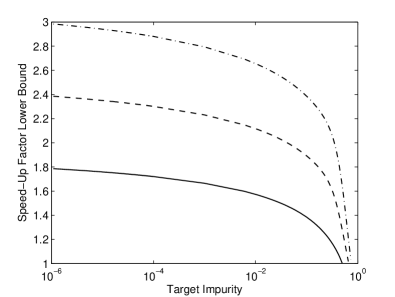
Figure 1: We plot here a lower bound on the speed-up factor provided by our feedback algorithm as a function of the target impurity, when the initial state is completely mixed. The solid line gives the result for system dimension $N=2$, the dashed line for $N=3$ and the dot-dashed line for $N=4$.

Before we finish we describe in a little more detail the feedback Hamiltonian involved in implementing the algorithm. To implement the feedback algorithm the controller is required to apply a unitary operation to the system so as to preserve the basis in which the density matrix, $\rho$, is diagonal, and, if necessary, apply a unitary operation to reorder the eigenvalues of $\rho$. To calculate the first unitary the controller diagonalizes $d\rho$. Since $d\rho$ has two terms, one proportional to $dt$ and the other to $dW$, this unitary will in general take the form $U(t,dt)=e^{i(H_{1}(t)dt+H_{2}(t)dW)}$ for some operators $H_{1}$ and $H_{2}$. The feedback Hamiltonian is thus, in general, $H(t)=H_{1}(t)+H_{2}(t)(dW/dt)$, and therefore contains a term proportional to the noise part of the measurement record $y(t)$. This kind of quantum feedback has been studied extensively by Wiseman and Milburn WM93 . The second unitary, that required to reorder the eigenvalues of $\rho$ should ideally perform the operation in a single time step. This requires a Hamiltonian proportional to $1/dt$, and since $dt$ should ideally be small on the time scale of the dynamics due to the measurement, this would require a Hamiltonian large compared to $\gamma$.

A number of interesting open questions remain. While we have found a lower bound on the performance of our algorithm, its actual performance may be higher. In addition, we do not know whether this algorithm is optimal. Further, in the above analysis we have focused on the ability of feedback to increase the speed of state-reduction under the assumption that there is no significant limitation on the feedback Hamiltonian. It will be interesting to consider the performance of the algorithm when specific limits are placed on the feedback Hamiltonian, and this will be the subject of future work.

Acknowledgements: The authors would like to thank Tanmoy Bhattacharya, Julia Kempe and Howard Wiseman for helpful discussions.

References

- (1) See, e.g. J. I. Cirac and P. Zoller, Phys. Rev. Lett. 74, 4091 (1995); B. E. Kane, Nature 393, 133 (1998); L. C. L. Hollenberg et al., Phys. Rev. B 69, 113301 (2004).
- (2) See, e.g. D. J. Tannor and A. Bartana, J. Phys. Chem. A 103, 10359-10363 (1999); S.E. Sklarz, D.J. Tannor and N. Khaneja, Phys. Rev. A 69, 053408 (2004).
- (3) V. P. Belavkin, Nondemolition measurements, nonlinear filtering and dynamic programming of non-linear stochastic processes. In A. Blaquiere (ed.), Modelling and control of systems, Lect. Notes in Control and Information Sciences 121, (Springer, Berlin, 1988) pp. 245-265.
- (4) H. M. Wiseman and G. J. Milburn, Phys. Rev. Lett. 70 548 (1993); H. M. Wiseman, Phys. Rev. A 49, 2133 (1994).
- (5) M. Yanagisawa and H. Kimura, in Learning, Control and Hybrid Systems, Lecture Notes in Control and Information Sciences Vol.241, 294 (Springer-Verlag, 1998).
- (6) A. C. Doherty and K. Jacobs, Phys. Rev. A 60, 2700 (1999).
- (7) A. C. Doherty, S. Habib, K. Jacobs, H. Mabuchi and S. M. Tan, Phys. Rev. A 62, 012105 (2000):
- (8) M.R. James, Phys. Rev. A, 69, 032108 (2004).
- (9) K. Jacobs, Phys. Rev. A 67, 030301(R) (2003); K. Jacobs, Proc. of SPIE 5468, 355 (2004).
- (10) C. A. Fuchs and K. Jacobs, Phys. Rev. A 63, 062305 (2001).
- (11) An introduction to continuous quantum measurement is given in Bxx . Other recent treatments of continuous measurements of Hermitian operators are given in DJ99 ; K00 , where the first uses the results of optical continuous measurements in C93 ; WM93 . A selection of the original work on continuous measurement is given in references B88 ; BS88 ; D86 ; B87 .
- (12) T. A. Brun, Am. J. Phys. 70, 719 (2002).
- (13) A. N. Korotkov, Phys.Rev.B 63, 115403 (2001).
- (14) H. J. Carmichael, S. Singh, R. Vyas and P. R. Rice, Phys. Rev. A, 39, 1200 (1989); H. Carmichael, An Open Systems Approach to Quantum Optics (Springer-Verlag, Berlin, 1993).
- (15) H. M. Wiseman and G. J. Milburn, Phys. Rev. A 47, 642 (1993).
- (16) V. P. Belavkin and P. Staszewski, Phys. Lett. A 40, 359 (1989).
- (17) L. Diosi, Phys. Lett. 114A, 451 (1986); L. Diosi, Phys. Lett. 132A, 233 (1988).
- (18) A. Barchielli, J. Phys A: Math. Gen. 20, 6341 (1987).
- (19) I. D. Ivanovic, J. Phys. A 14, 3241 (1981); W. K. Wootters and B. D. Fields, Annals of Physics 191, 363 (1989).
- (20) We use to denote the impurity because it is sometimes referred to as the linear entropy.
- (21) K. Jacobs and P. L. Knight, Phys. Rev. A. 57, 2301 (1998).
- (22) R. Bhatia,“Matrix Inequalities”, (Springer, Berlin, 1997).