Quantum entanglement dynamics and decoherence wave in spin chains at finite temperatures

Abstract

We analyze the quantum entanglement at the equilibrium in a class of exactly solvable one-dimensional spin models at finite temperatures and identify a region where the quantum fluctuations determine the behavior of the system. We probe the response of the system in this region by studying the spin dynamics after projective measurement of one local spin which leads to the appearance of the “decoherence wave”. We investigate time-dependent spin correlation functions, the entanglement dynamics, and the fidelity of the quantum information transfer after the measurement.

I Introduction

Collective behavior in many-body quantum systems is associated with the development of classical correlations, as well as of the correlations which cannot be accounted for in terms of classical physics, namely, entanglement. The entanglement represents in essence the impossibility of giving a local description of a many-body quantum state. Experimental tests of the nonlocality by means of the Bell-type inequality 1 have been made with different kind of particles including photons 2 and massive fermions 3 ; 4 ; 44 . The entanglement is expected to play an essential role at quantum phase transitions 5 , where quantum fluctuations manifest themselves at all length scales. Several groups investigated this problem by studying the quantum spin systems (see, e.g., Refs.Osbo02, ; 19, ; Hami05, ; 12, ; 14, ; 24, ; 25, ; 26, ; 27, ; 28, ; 29, ; 30, ; 31, ; 32, ; Amic04, ; Subr05, ; ghos1, ). Additional studies have been carried out for more complicated systems including both itinerant electrons and localized spins; the local entanglement for these systems have been discussed in a context of the quantum phase transitions gu ; Anfo and of the Kondo problem ourkondo . In particular, Anfossi et al Anfo performed, within the density-matrix renormalization group method, a numerical comparison between the standard finite-size scaling and the local entanglement for the Hubbard model in a presence of bond charge interaction (the Hirsch model) at the Mott metal-insulator transition. Katsnelson et al ourkondo have considered the suppression of the Kondo resonance by a probing of the charge state of the magnetic impurity which leads to the partial destruction of the entanglement between the localized spin and itinerant-electron Fermi sea. These examples illustrate a relevance of the concept of entanglement for the many-body physics. Moreover, the entanglement overwhelmingly comes into play in the quantum computation and communication theory 6 , being the main physical resource needed for their specific tasks. The essential idea is to encode one particular qubit, and let it be transported to across the chain to recover the code from another qubit some distance away 7 .

The suppression of the entanglement by decohering actions such as noise, measurements, etc., is one of the central problems in quantum computation and quantum information theory; therefore the concept of entanglement for mixed states is of primary relevance Benn96 . For example, it is important to know what happens with the quantum computer after the measurement of one qubit state; for the case of the quantum system with broken continuous symmetry such as Bose-Einstein condensate (BEC) or easy-plane antiferromagnet the local measurements lead to the formation of the “decoherence wave” ourbec ; ourneel . It is interesting to investigate the effect of the decoherence wave on the entanglement in the system.

Motivated by these results, in this paper, we aim on the evaluation of the pairwise entanglement in the 1D Ising-XY model with transverse magnetic field at finite temperatures. We identify a region where the thermal entanglement is non zero while it is zero at zero temperature, which results from the entanglement of the excited states as it will be explained below (section II). We study the dynamical response of the system in the non vanishing entanglement region, which is the useful region for quantum information processing, after a projective measurement on one local spin. We find that, similar to the case of the BEC considered earlier ourbec the spin decoherence wave appears propagating with the velocity proportional to the interaction strength. We investigate also the zero temperature case studying the time-dependent correlation functions and we discuss the relation between the dynamics of the magnetization and the entanglement (section III). Our conclusions are given in section IV.

II Thermal entanglement in the Ising-XY Model with transverse field

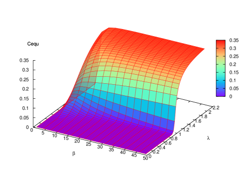
Fig. 1: (color online) Pairwise entanglement for the nearest neighbors in the isotropic XY model with transverse field at the equilibrium as function of $\beta$ and $\lambda$. Cequ is defined by Eq.(12) for the thermodynamic equilibrium state.

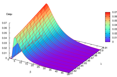
Fig. 2: (color online)Same as Fig. 1 for $0.8<\lambda<0.9$.

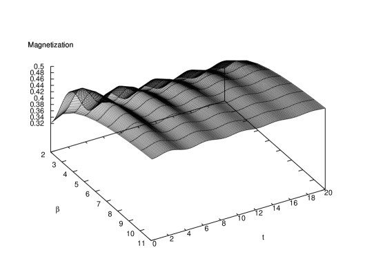
Fig. 3: Site magnetization as function of the temperature and time with $m-l=1$ and $\lambda=0.8$.

In this section we present the solution of the N-sites Ising-XY model with transverse field following the standard method Lieb61 ; Baro70 . We proceed with the Hamiltonian

$${\cal H}=-\sum_{i=1}^{N}(\lambda[(1+\gamma)\sigma_{i}^{x}\sigma_{i+1}^{x}+(1-\gamma)\sigma_{i}^{y}\sigma_{i+1}^{y}]+\sigma_{i}^{z})\,,$$ (1)

where $\sigma^{a}_{i}$ are the Pauli operators, obeying the usual commutation relations $[\sigma^{a}_{i},\sigma^{b}_{j}]=2i\epsilon^{abc}\delta^{ij}\sigma^{c}_{i}$ . The Zeeman energy in the external magnetic field, as well as the Planck constant $\hbar$, have been set to 1. We assume cyclic boundary conditions, i.e., the index $i$ in the sum (1) runs over ${1\dots N}$ with $S_{N+1}=S_{1}$. This Hamiltonian can be diagonalized by means of the Jordan-Wigner transformation Lieb61 ; Baro70 that maps spins to one-dimensional spinless fermions with creation and annihilation operators $c_{i}$ and $c_{i}^{{\dagger}}$. The Hamiltonian Eq.(1) in the fermionic operator representation is represented by the quadratic form

$$H=(\sum_{i,j}c_{i}^{{\dagger}}A_{i,j}c_{j}+\frac{1}{2}[c_{i}^{{\dagger}}B_{i,j}c_{j}^{{\dagger}}+{\rm H.c.}])+N\,,$$ (2)

where $A_{i,i}=-1$ and $A_{i,i+1}=-\frac{1}{2}\lambda=A_{i+1,i}$, $B_{i,i+1}=-\frac{1}{2}\lambda\gamma=-B_{i+1,i}$, and all other $A_{i,j}$ and $B_{i,j}$ are zero. The quadratic Hamiltonian (2) can be diagonalized by a linear Bogoliubov transformation of the fermionic operators,

$$\eta_{k}=\sum_{i}(g_{ki}c_{i}+h_{ki}c_{i}^{{\dagger}})\,,$$ (3)

$$\eta_{k}^{{\dagger}}=\sum_{i}(g_{ki}c_{i}^{{\dagger}}+h_{ki}c_{i})\,,$$ (4)

where the $g_{ki}$ and $h_{ki}$ can be chosen to be real. After that it takes the diagonal form

$$H=\sum_{k}\Lambda_{k}\eta_{k}^{{\dagger}}\eta_{k}-\frac{1}{2}\Lambda_{k}\,,$$ (5)

where

$$\Lambda_{k}=\sqrt{(\gamma\lambda\sin k)^{2}+(1+\lambda\cos k)^{2}}\,.$$ (6)

After the diagonalization of the Hamiltonian now we can proceed with the evaluation of the thermal pairwise entanglement. The pairwise entanglement, as its name indicates, measures how two spins separated by a distance $r$ are entangled. This measure is to be accomplished by evaluating the pairwise entanglement of the two-site density matrix after tracing out all other spins in the chain. We evaluate the entanglement of this states by using the concurrence which is defined as Benn96

$${\cal C}=\max\{\lambda_{1}-\lambda_{2}-\lambda_{3}-\lambda_{4},0\}\,,$$ (7)

where $\lambda$’s are the square roots of the eigenvalues in decreasing order of the matrix $\rho_{AB}(\sigma_{y}\otimes\sigma_{y}\rho_{AB}^{\star}\sigma_{y}\otimes\sigma_{y})$, where $\rho_{AB}^{\star}$ is the corresponding complex conjugation in the computational basis $\{|++\rangle,|+-\rangle,|-+\rangle,|--\rangle\}$. As usual, at the thermal equilibrium the system is described by the canonical ensemble density matrix

$$\rho=\frac{e^{-\beta H}}{Z}\,,$$ (8)

where $Z={\rm Tr}e^{-\beta H}$ is the partition function of the system. Thus the reduced two-site density matrix, after taking into account the symmetries consideration, assumes the following form

$$\rho_{ij} = {\rm Tr}_{k\neq i,j}\frac{e^{-\beta H}}{Z}=\frac{1}{4}(I\otimes I+\langle\sigma_{z}\rangle(\sigma_{z}^{i}\otimes I+I\otimes\sigma_{z}^{j})$$ (9)

$$+ \sum_{k=1}^{3}\langle\sigma^{i}_{k}\sigma^{j}_{k}\rangle\sigma^{i}_{k}\otimes\sigma^{j}_{k})\,.$$

The correlation functions that show up in the density matrix Eq.(9) are well known Baro70 and for the nearest neighbor case considering here these correlation functions are giving by

$$\langle\sigma^{i}_{x}\sigma^{j}_{x}\rangle={\cal G}_{-1},\quad\langle\sigma^{i}_{y}\sigma^{j}_{y}\rangle={\cal G}_{1},\quad\langle\sigma^{i}_{x}\sigma^{j}_{x}\rangle=\langle\sigma_{z}\rangle^{2}-{\cal G}_{1}{\cal G}_{-1},$$

$$\quad\langle\sigma_{z}\rangle=-{\cal G}_{0}\,,$$ (10)

with

$${\cal G}_{mi} = \frac{1}{\pi}\int_{0}^{\pi}dk\cos[k(m-i)](1+\lambda\cos k)\frac{\tanh(\Lambda_{k}\beta/2)}{\Lambda_{k}}$$ (11)

$$- \frac{\lambda\gamma}{\pi}\int_{0}^{\pi}dk\sin[k(m-i)]\sin k\frac{\tanh(\Lambda_{k}\beta/2)}{\Lambda_{k}}\,$$

Thus the concurrence for the case of isotropic XY model, $\gamma=0$, reads

$${\cal C}=\max\{0,||{\cal G}_{1}|-\sqrt{\frac{1}{4}(1+{\cal G}_{0}^{2}-{\cal G}_{1}^{2})^{2}-{\cal G}_{0}^{2}}|\}\,,$$ (12)

and at $T=0$ we have ${\cal G}_{0}=1$ and

$${\cal G}_{1}=\left\{\begin{array}[c]{cc}0&\quad{\lambda\leq 1}\\ \frac{2}{\pi}\sqrt{1-\lambda^{-2}}&\quad\lambda>1\end{array}\right.\,.$$

The two-site entanglement between the nearest-neighbors for the isotropic XY model is shown in Fig.1. One can see from this figure that there is a region where the entanglement increases with the temperature increase whereas for $\lambda\leq 1$ the entanglement is zero at zero temperature and it remains zero until a critical temperature where the system starts to be entangled. Fig.2 displays with more details a relevant region with $0.8<\lambda<0.99$. It is clearly seen in this figure that there is a strong enough entanglement in the region $2<\beta<20$, however, outside this region no entanglement can be observed. This entanglement transition should be understood as an effect of the entanglement of the higher excited states. Note that the ground state in this case is unentangled with all spins pointed in the same direction. Similar observation has been made in Refs.Osbo02, and 31, . In the region where the entanglement does not vanish we expect the quantum fluctuations likely to dominate the behavior of the system and it is the region where the quantum information processing should be studied since it is well know that the entanglement is the main resource for quantum information. Thus the study of the dynamics of entanglement for this region is relevant. In the next section we will study the response of the system after a projective measurement in this region.

III Spin decoherence after a projective measurement

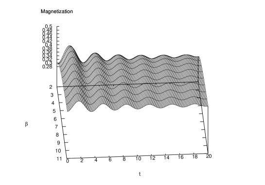
Fig. 4: Site magnetization as function of the temperature and time with $m-l=1$ and $\lambda=0.99$.

Fig. 5: Site magnetization as function of the temperature and time with $m-l=1$ and $\lambda=0.8$ for the case without knowledge of the measurement outcome.

Fig. 6: Site magnetization as function of the site location $x=m-l$ and time at fixed $\beta=10$ and $\lambda=2$.

As mentioned above we will study the consequences of the local projective measurement and analyze the system behavior in terms of the spin decoherence wave. We introduce the operators

$$A_{i}=c_{i}^{{\dagger}}+c_{i}\,\quad B_{i}=c_{i}^{{\dagger}}-c_{i}\,.$$ (13)

After a selective projective measurement with the projector $P=\frac{\sigma_{z}^{l}+1}{2}=\frac{1-A_{l}B_{l}}{2}$ ($P=P^{{\dagger}}$), which means that the positive $z$ direction of the local spin $l$ is the measurement result (a general measurement will be considered below), the mean value at time $t$ for an operator $A$ reads Hami04

$$\langle A(t)\rangle=\frac{{\rm Tr}\rho PA(t)P}{{\rm Tr}P\rho P}\,,$$ (14)

where $A(t)=e^{iHt}A(0)e^{-iHt}$. Since we are interested in the evaluation of the time-dependent average value of the magnetization in the $z$ direction at site $m$ we have $A(0)=\sigma_{z}/2=-\frac{A_{m}B_{m}}{2}$. In order to evaluate $\langle A(t)\rangle$ we write the operator $A_{i}$, and $B_{i}$ in term of $\eta$ and $\eta{{\dagger}}$ operators using the inverse transformation of Eqs.(3),(4). Since the Hamiltonian is diagonal being written in terms of $\eta$ operators we have

$$\eta^{{\dagger}}_{k}(t)=\exp{(i\Lambda_{k}t)}\eta_{k}^{{\dagger}}(0)\,.$$ (15)

Thus after a straightforward little algebra we found the following expression for $A(t)$

Fig. 7: Site magnetization at distance $x$ from the measurement point.

$$A(t)=\frac{-1}{2}\sum_{ii^{\prime}}\alpha_{ii^{\prime}}^{m}A_{i}A_{i^{\prime}}+\beta_{ii^{\prime}}^{m}A_{i}B_{i^{\prime}}+\gamma_{ii^{\prime}}^{m}B_{i}B_{i^{\prime}}\,,$$ (16)

where

$$\alpha_{ii^{\prime}}^{m}=\phi_{mi}G_{mi^{\prime}};\,\beta_{ii^{\prime}}^{m}=\phi_{mi}\psi_{mi^{\prime}}-G_{mi}G_{mi^{\prime}};\,\gamma_{ii^{\prime}}^{m}=G_{mi}\psi_{mi^{\prime}}\,,$$ (17)

and in the thermodynamic limit ($N\rightarrow\infty$) we have

$$\phi_{\mu\nu}=\psi_{\mu\nu}=\frac{1}{\pi}\int_{0}^{\pi}dk\cos k(\mu-\nu)\cos(\Lambda_{k}t)\,,$$ (18)

$$G_{\mu\nu} = \frac{i}{\pi}\int_{0}^{\pi}dk\cos[k(\mu-\nu)](1+\lambda\cos k)\frac{\sin(\Lambda_{k}t)}{\Lambda_{k}}$$ (19)

$$- \frac{i\lambda\gamma}{\pi}\int_{0}^{\pi}dk\sin[k(\mu-\nu)]\sin k\frac{\sin(\Lambda_{k}t)}{\Lambda_{k}}\,.$$

We define the operator ${\cal A}=\sum_{ii^{\prime}}\beta_{ii^{\prime}}^{m}A_{i}B_{i^{\prime}}$ which corresponds to the part of $A(t)$ with real coefficients. Clearly we have $\langle{\cal A}\rangle_{\beta}=\langle A\rangle_{\beta}$, therefore after some calculations we obtain

$$\langle A\rangle_{\beta} = \frac{1}{4({\cal G}_{ll}+1)}\left.({\cal G}_{mm}+\sum_{ii^{\prime}}\beta_{ii^{\prime}}^{m}[\langle A_{l}B_{l}A_{i}B_{i^{\prime}}\rangle_{\beta}\right.$$ (20)

$$+ \left.\langle A_{i}B_{i^{\prime}}A_{l}B_{l}\rangle_{\beta}-\langle A_{l}B_{l}A_{i}B_{i^{\prime}}A_{l}B_{l}\rangle_{\beta}\right.])\,,$$

where

$$\langle A_{l}B_{l}A_{i}B_{i^{\prime}}\rangle_{\beta}={\cal G}_{ii^{\prime}}{\cal G}_{ll}+\delta_{il}\delta_{i^{\prime}l}-{\cal G}_{li}{\cal G}_{li^{\prime}}\,,$$ (21)

$$\langle A_{i}B_{i^{\prime}}A_{l}B_{l}\rangle_{\beta}={\cal G}_{ii^{\prime}}{\cal G}_{ll}+\delta_{il}\delta_{i^{\prime}l}-{\cal G}_{il}{\cal G}_{i^{\prime}l}\,,$$ (22)

$$\langle A_{l}B_{l}A_{i}B_{i^{\prime}}A_{l}B_{l}\rangle_{\beta}=-4\delta_{li^{\prime}}\delta_{il}{\cal G}_{ll}+\delta_{li}({\cal G}_{i^{\prime}l}+{\cal G}_{li^{\prime}})+\delta_{li^{\prime}}({\cal G}_{il}+{\cal G}_{li})+{\cal G}_{ll}{\cal G}_{i^{\prime}l}({\cal G}_{il}-{\cal G}_{li})+{\cal G}_{ll}{\cal G}_{li^{\prime}}({\cal G}_{li}-{\cal G}_{il})-{\cal G}_{ii^{\prime}}\,.$$ (23)

Here we have used the Fermi distribution function

$$\langle\eta_{k}\eta^{{\dagger}}_{k^{\prime}}\rangle=\frac{\delta_{kk^{\prime}}}{e^{-\beta\Lambda_{k}}+1}\,.$$ (24)

For simplicity, in this paper we will further consider only the isotropic XY Model, $\gamma=0$; the case $\gamma\neq 0$ will be addressed in the future. Thus, the magnetization at the site $m$ in the $z$ direction can be written as follow

$$\langle{A}\rangle_{\beta}=\frac{1}{4({\cal G}_{ll}+1)}\left\{{\cal G}_{mm}+(2{\cal G}_{ll}+1)[2(\phi_{ml}^{2}-G_{ml}^{2})+\alpha-\alpha^{\prime}]\right.+\left.4(G_{ml}\beta_{ml}^{\prime}-\phi_{ml}\beta_{ml})+2(\beta^{\prime 2}_{ml}-\beta_{ml}^{2})\right\}\,,$$ (25)

where the expressions of $\alpha,\,\beta_{ml},\,\alpha^{\prime},\,\beta_{ml}^{\prime}$ are given in the Appendix.

The magnetizations at the neighboring site $m-l=1$ for the cases $\lambda=0.8$ and $\lambda=0.99$ are shown in Figs.3 and 4, respectively, as functions of the inverse temperature $\beta$ and of the time. The magnetization oscillate in time with the frequency proportional to $\lambda$ which is a result of the propagation of the decoherence wave after the local measurement ourbec . One can see that the amplitude of these oscillations increases in the close vicinity of the quantum critical point $\lambda=1$. Figs.3 and 4 demonstrate also that the amplitude increases with the temperature increase. It is connected probably with the thermal entanglement in the system under consideration (see the previous section).

For a complete von Neumann measurement 6 without knowledge of the measurement outcome the mean value for the operator $A$ at time $t$ is

$$\langle A(t)\rangle={{\rm Tr}\rho PA(t)P}+{{\rm Tr}\rho(1-P)A(t)(1-P)}\,,$$ (26)

Thus we have

$$\langle{A}\rangle_{\beta} = \frac{1}{4}\left\{{\cal G}_{mm}+4{\cal G}_{ll}(\phi_{ml}^{2}-G_{ml}^{2})+(\alpha-\alpha^{\prime})\right.$$ (27)

$$+ \left.4(G_{ml}\beta_{ml}^{\prime}-\phi_{ml}\beta_{ml})\right\}\,,$$

The magnetization at the neighboring site $m-l=1$ after the measurement is plotted in Fig.5 for $\lambda=0.8$ as a function of $\beta$ and the time. One can clearly see from this figure that there is a reduction of the amplitude of the oscillation with respect to the selective measurement; this effect is due to the mixing of the state as here we don’t know the results of the measurement outcome. Fig.6 displays the propagation of the decoherence wave, that is, the magnetization distribution as a function of the distance from the measured site $x$ and time $t$ at a fixed value of $\beta=10$ and $\lambda=2$.

Fig. 8: Single-site entanglement $S$ at distance $x$ from the measurement point.

Fig. 9: Two-site entanglement C between the site $m$ and the site $i$ at zero temperature with $x=i-m$.

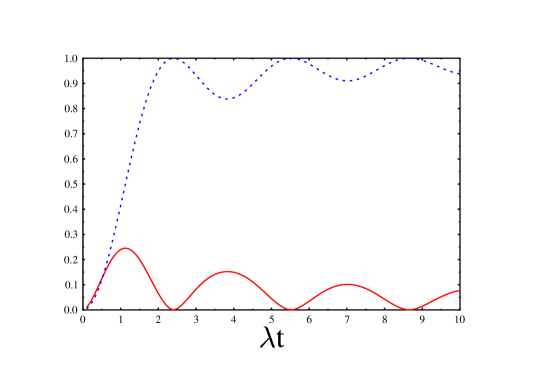
Fig. 10: (color online) $\langle\sigma_{z}\rangle$ (dotted line) and single site entanglement (solid line) are shown at the site $m$.

Fig. 11: The fidelity of the quantum channel is shown at site $i$.

Now we consider the effect of the local measurement on the pairwise entanglement in the system. This require the evaluation of a correlations functions such as $\langle\sigma_{i}^{\alpha}\sigma_{j}^{\beta}\rangle$. Here we will present the results for an interesting particular case, namely, for $\lambda<1$ and at zero temperature. Then, there is no entanglement in the system before the measurement since all spin are pointing in the same $z$-direction in the ground state. Therefore a projective measurement of the $z$-component of the magnetization will not provide us any nontrivial information and will not generate entanglement. However, we will show that the projective measurement of the $x$-component does create the entanglement. After the projective measurement in the $x$ direction at site $m$ with positive outcome the wave function will be

$$|\Psi\rangle_{m}=\frac{1+c_{m}^{{\dagger}}}{\sqrt{2}}|vac\rangle\,.$$ (28)

At time $t$ we have

$$c^{{\dagger}}_{m}(t)=\sum_{l}(G_{ml}+\phi_{ml})c^{{\dagger}}_{l}=\sum_{l}w_{l}(t)c^{{\dagger}}_{l}\,,$$ (29)

where in the thermodynamics limit $w_{l}(t)=J_{m-l}(\lambda t)$ and $J_{n}(x)$ is the Bessel function of order $n$. Thus the time-dependent wave function after the measurement will be

$$|\Psi_{m}(t)\rangle=\frac{1+\sum_{l}w_{l}(t)c_{l}^{{\dagger}}}{\sqrt{2}}|vac\rangle\,,$$ (30)

Thus, the time-dependent two-spin density matrix can be written in the form

$$\rho_{ij}=\frac{1}{2}\left(\begin{array}[c]{cccc}0&0&0&0\\ 0&w_{i}^{2}&w_{i}w_{j}&w_{i}\\ 0&w_{i}w_{j}&w_{j}^{2}&w_{j}\\ 0&w_{i}&w_{j}&2-w_{i}^{2}-w_{j}^{2}\end{array}\right)\,,$$

and the corresponding one-particle density matrix is $\rho_{i}=\frac{1}{2}\left(\begin{array}[c]{cc}w_{i}^{2}&w_{i}\\ w_{i}&2-w_{i}^{2}\end{array}\right)\,.$ The magnetization of the site $i$ is therefore given by $\langle\sigma_{z}\rangle/2={\rm Tr}\rho\sigma_{z}/2=(w_{i}^{2}-1)/2$. The single-site entropy, $S(\rho_{i})=-{\rm Tr}\rho_{i}\log\rho_{i}$, which characterizes the entanglement of one spin with the rest of the chain, can also be evaluated in this case. The pairwise entanglement for the two-site density matrix can be evaluated using Eq.(7). A straightforward algebra lead to the following expression for the concurrence:

$${\cal C}=w_{i}w_{j}\,.$$ (31)

In Figs.7, 8, 9 we show the single-spin quantum entropy and the magnetization at distance $x$ from the measurement point, as well as the pairwise entanglement between site $m$ and $i$ as functions of time and of $x=i-m$. We conclude from these figures that the single-site entanglement and the pairwise entanglement propagate with the velocity proportional to the interaction strength, like the spin decoherence wave. In Fig.10 we display the site magnetization together with the single-site entanglement which demonstrates clearly that these two quantities oscillate coherently. This confirms that the dynamics of the spin decoherence reflects in some sense the dynamics of the entanglement in the system.

The fidelity of the communication at site $m$ through the channel is the probability that a channel output pass a test for being the same as the input conducted by someone who knows what the input was. It can be defined as Benn196

$$F={\langle}\psi_{m}|\rho_{i}|\psi_{m}\rangle=\frac{1+w_{i}}{2}\,,$$ (32)

where $|\psi_{m}\rangle=\frac{|0\rangle+|1\rangle}{\sqrt{2}}$ is the state of the site $m$ right after the measurement. In fact, the spin chain acts as an amplitude damping quantum channel where the initial state is transformed under the action of the superoperator $ to 6

$$\rho\rightarrow\$(\rho)=M_{0}\rho M_{0}^{{\dagger}}+M_{1}\rho M_{1}^{{\dagger}}\,,$$ (33)

with the Kraus operators such $M_{0}=\left(\begin{array}[c]{cc}w_{i}&0\\ 0&1\end{array}\right)\,,$ and $M_{1}=\left(\begin{array}[c]{cc}0&0\\ \sqrt{1-\omega_{i}^{2}}&0\end{array}\right)\,$ where as usual $M_{1}$ describe the quantum jump and $M_{0}$ represent no quantum jump. The fidelity of the channel is shown in Fig.11. One can see clearly from this figure that the channel can be efficiently used to transmit the quantum information. The fidelity has a maximum value for $x=i-m\sim\lambda t$. This means that the quantum state is transported with the velocity proportional to the interaction strength $\lambda$ similar to the decoherence wave. After a time $t=x/\lambda$ the state can be recovered with maximum fidelity at a distance $x$ from the initial site $m$.

IV Conclusions

In this paper, we have evaluated the equilibrium pairwise entanglement at finite temperatures in the isotropic one-dimensional Ising-XY model with transverse magnetic field. Our findings indicate that the behavior of entanglement with respect to temperature, at least for moderate values of temperature, is quite complex. In particular, we have found that for some ranges of temperature, entanglement in the system can grow with increasing temperature, which results from the entanglement of the excited states. We have studied the dynamical response of the system in a relevant region for quantum information processing after a projective measurement on one local spin which leads to the appearance of the “decoherence wave” that propagate with velocity proportional to the coupling constant $\lambda$, similar to the case of the Bose-Einstein condensate studied earlier ourbec . One motivation behind our study is to know what happens with the quantum computer after the measurement. We have investigated for specific case ($T=0$ and $\lambda<1$) the dynamics of the entanglement and the spin decoherence wave and we have found that those quantities propagates coherently through the chain with the same velocity that is proportional to $\lambda$. The fidelity of the channel has been shown to be represented as amplitude damping channel. Finally, a generalization to $\gamma\neq 0$ and study of the entanglement dynamics in such system are desirable.

Appendix

Using the standard properties of the Fourier transformation, one has

$$\sum_{l}G_{il}\bar{G}_{i^{\prime}l}=\sum_{l}\int_{-\pi}^{\pi}\frac{dk}{2\pi}G(k)e^{ik(i-l)}\int_{-\pi}^{\pi}\frac{dk^{\prime}}{2\pi}\bar{G}(k^{\prime})e^{ik^{\prime}(i^{\prime}-l)}=\int_{-\pi}^{\pi}\frac{dk}{2\pi}G(k)\bar{G}(-k)e^{ik(i-i^{\prime})}$$ (34)

Putting $\gamma=0$ we find

$$\alpha = \sum_{ii^{\prime}}\phi_{mi}\phi_{mi^{\prime}}{\cal G}_{ii^{\prime}}=\frac{1}{\pi}\int_{0}^{\pi}dk(1+\lambda\cos k)\frac{\tanh(\Lambda_{k}\beta/2)}{\Lambda_{k}}\cos^{2}(\Lambda_{k}t)$$

$$\beta_{ml} = \sum_{i}\phi_{mi}{\cal G}_{li}=\frac{1}{\pi}\int_{0}^{\pi}dk\cos[k(m-l)](1+\lambda\cos k)\frac{\tanh(\Lambda_{k}\beta/2)}{\Lambda_{k}}\cos(\Lambda_{k}t)$$

$$\alpha^{\prime} = \sum_{ii^{\prime}}G_{mi}G_{mi^{\prime}}{\cal G}_{ii^{\prime}}=\frac{-1}{\pi}\int_{0}^{\pi}dk(1+\lambda\cos k)^{3}\frac{\tanh(\Lambda_{k}\beta/2)}{\Lambda_{k}^{3}}\sin^{2}(\Lambda_{k}t)$$

$$\beta_{ml}^{\prime} = \sum_{i}G_{mi}{\cal G}_{li}=\frac{i}{\pi}\int_{0}^{\pi}dk\cos[k(m-l)](1+\lambda\cos k)^{2}\frac{\tanh(\Lambda_{k}\beta/2)}{\Lambda_{k}^{2}}\sin(\Lambda_{k}t)$$

References

- (1) J. S. Bell, Physics 1, 195 (1964); Rev. Mod. Phys. 38, 447 (1966).
- (2) A. Aspect, Nature (London) 398, 189 (1999).
- (3) M. Lamehi-Rachti and W. Mittig, Phys. Rev. D 14, 2543 (1976).
- (4) C. Polachic, C. Rangacharyulu, A.M. van den Berg, S. Hamieh, M.N. Harakeh, M. Hunyadi, M.A. de Huu, H.J. Wörtche, J. Heyse, C. Baumer., D. Frekers, S.Rakers, J.A. Brooke and P. Busch, Phys. Lett. A 323, 176 (2004).
- (5) S. Hamieh, H.J. Wörtche, C. Baumer, A.M. van den Berg, D. Frekers, M.N. Harakeh, J. Heyse, M. Hunyadi, M.A. de Huu, C. Polachic and C. Rangacharyulu, J. Phys. G 30, 481 (2004).
- (6) S. Sachdev, Quantum Phase Transitions (Cambridge University Press, Cambridge, 1999).
- (7) T. Osborne and M. Nielsen, Phys. Rev. A 66, 032110 (2002).
- (8) A. Osterloh, L. Amico, G. Falci, and R. Fazio, Nature (London) 416, 608 (2002).
- (9) S. Hamieh and A. Tawfik, Acta Phys. Polon. B 36, 801 (2005).
- (10) M. A. Nielsen, Ph.D. thesis, University of New Mexico, 1998; quant-ph/0011036.
- (11) P. Zanardi and X. Wang, J. Phys. A 35, 7947 (2002).
- (12) X. Wang, H. Fu, and A. I. Solomon, J. Phys. A 34, 11307 (2001).
- (13) W. K. Wootters, Contemporary Mathematics 305, 299 (2002).
- (14) M. C. Arnesen, S. Bose, and V. Vedral, Phys. Rev. Lett. 87, 017901 (2001).
- (15) D. A. Meyer and N. R. Wallach, J. Math. Phys. 43, 4273 (2002).
- (16) D. Gunlycke, S. Bose, V. M. Kendon, and V. Vedral, Phys. Rev. A 64, 042302 (2001).
- (17) X. Wang, Phys. Rev. A 64, 012313 (2001).
- (18) H. Fu, A. I. Solomon, and X. Wang, J. Phys. A 35, 4293 (2002).
- (19) X. Wang, Phys. Lett. A 281, 101 (2001).
- (20) X. Wang and P. Zanardi, Phys. Lett. A 301, 1 (2002).
- (21) L. Amico, A. Osterloh, F. Plastina, R. Fazio, and G. M. Palma, Phys. Rev. A 69, 022304 (2004).
- (22) V. Subrahmanyam and A. Lakshminarayan, quant-ph/0409048; V. Subrahmanyam, Phys. Rev. A 69, 022311 (2004); V. Subrahmanyam, Phys. Rev. A 69, 034304 (2004).
- (23) S. Ghosh, T. F. Rosenbaum, G. Aeppli, and S. N. Coppersmith, Nature (London) 425, 48 (2003).
- (24) S. Gu, S. Deng, Y. Li, and H. Lin, Phys. Rev. Lett. 93, 086402 (2004).
- (25) A. Anfossi, C. Boschi, A. Montorsi, and F. Ortolani, cond-mat/0503600.
- (26) M. I. Katsnelson, V. V. Dobrovitski, H. A. De Raedt, and B. N. Harmon, Phys. Lett. A 318, 445 (2003).
- (27) M. Nielsen and I. Chuang, Quantum Computation and Quantum Information (Cambridge University Press, Cambridge, 2000).
- (28) S. Bose, Phys. Rev. Lett. 91, 207901 (2003).
- (29) C. Bennett, D. DiVincenzo, J. Smolin, and W. Wootters, Phys. Rev. A 54, 3824 (1996); S. Hill and W. Wootters, Phys. Rev. Lett. 78, 5022 (1997); W. Wootters, Phys. Rev. Lett. 80, 2245 (1998).
- (30) M. I. Katsnelson, V. V. Dobrovitski, and B. N. Harmon, Phys. Rev. A 62, 022118 (2000).
- (31) M. I. Katsnelson, V. V. Dobrovitski, and B. N. Harmon, Phys. Rev. B 63, 212404 (2001).
- (32) E. Lieb, T. Schultz, and D. Mattis, Ann. Phys. (N.Y.) 60, 407 (1961).
- (33) E. Barouch and B. McCoy, Phys. Rev. A 2, 1075 (1970); E. Barouch and B. McCoy, Phys. Rev. A 3, 786 (1971).
- (34) S. Hamieh, R. Kobes, and H. Zaraket, Phys. Rev. A 70, 052325 (2004).
- (35) C. Bennett, H. Bernstein, S. Popescu, and B. Schumacher, Phys. Rev. A 53, 2046 (1996).