Quantum Arnol’d diffusion in a rippled waveguide

Abstract

We study the quantum Arnol’d diffusion for a particle moving in a quasi-1D waveguide bounded by a periodically rippled surface, in the presence of the time-periodic electric field. It was found that in a deep semiclassical region the diffusion-like motion occurs for a particle in the region corresponding to a stochastic layer surrounding the coupling resonance. The rate of the quantum diffusion turns out to be less than the corresponding classical one, thus indicating the influence of quantum coherent effects. Another result is that even in the case when such a diffusion is possible, it terminates in time due to the mechanism similar to that of the dynamical localization. The quantum Arnol’d diffusion represents a new type of quantum dynamics, and may be experimentally observed in measurements of a conductivity of low-dimensional mesoscopic structures.

As is well known, one of the mechanisms of the dynamical chaos in the Hamiltonian systems is due to the interaction between nonlinear resonances [1]. When the interaction is strong, this leads to the so-called global chaos which is characterized by a chaotic region spanned over the whole phase space of a system, although large isolated islands of stability may persist. For a weak interaction, the chaotic motion occurs only in the vicinity of separatrices of the resonances, in accordance with the Kolmogorov-Arnol’d-Moser (KAM) theory (see, for example, Ref. [2]). In the case of two degrees of freedom ($N=2$), the passage of a trajectory from one stochastic region to another is blocked by KAM surfaces.

The situation changes drastically in many-dimensional ($N>2$) systems for which the KAM surfaces no longer separate stochastic regions surrounding different resonances, and chaotic layers of the destroyed separatrices form a stochastic web that can cover the whole phase space. Thus, if the trajectory starts inside the stochastic web, it can diffuse throughout the phase space. This weak diffusion along stochastic webs was predicted by Arnol’d in 1964 [3], and since that time it is known as a very peculiar phenomenon, however, universal for many-dimensional nonlinear Hamiltonian systems (see, for example, review [4] and references therein).

Recently, much attention has been paid to the chaotic dynamics of a particle in a rippled channel (see, for example, Refs. [5, 6, 7, 8, 9]). The main interest was in the quantum-classical correspondence for the conditions of a strong chaos. Specifically, in Ref. [5] the transport properties of the channel in a ballistic regime were under study. Energy band structure, the structure of eigenfunctions and density of states have been calculated in [6, 7]. The quantum states in the channel with rough boundaries, as well as the phenomena of quantum localization have been analyzed in [9]. The influence of an external magnetic field for narrow channels was investigated in [8]. These studies may have a direct relevance to the experiments with periodically modulated conducting channels. In this connection one can mention the investigation  [10] of transport properties of a mesoscopic structure (sequence of quantum dots) with the periodic potential formed by metallic gates.

In contrast with the previous studies, below we address the regime of a weak quantum chaos which occurs along the nonlinear resonances in the presence of an external periodic electric field. Our goal is to study the properties of the quantum Arnol’d diffusion which may be observed experimentally. The approach we use is based on the theory developed in Ref.[11] by making use of a simple model of two coupling nonlinear oscillators, one of which is driven by two-frequency external field.

We study the Arnol’d diffusion in a periodic quasi-one dimensional waveguide with the upper profile given in dimensionless variables by the function $y=d+a\cos{x}$. Here $x$ and $y$ are the longitudinal and transverse coordinates, $d$ is the average width, and $a$ is the ripple amplitude. The low profile is assumed to be flat, $y=0$. The nonlinear resonances arise due to the coupling between two degrees of freedom, with the following resonance conditions,

$$\eta=T_{x}/T_{y}=\omega_{y}/\omega_{x}$$ (1)

Here $T_{y}$ is the period of a transverse oscillation inside the channel, $T_{x}$ is the time of flight of a particle over one period of the waveguide, $\omega_{x}$ and $\omega_{y}$ are the corresponding frequencies, and $\eta$ is the rational number.

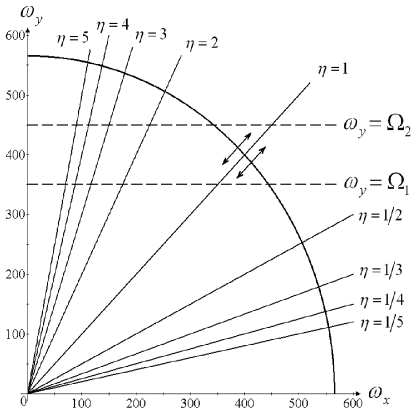
FIG. 1.: Some of the coupling resonances for different values of $\eta$, with the isoenergetic curve $E=160000$ in the frequency plane. The locations of resonances are shown by dashed lines.

The mechanism of the classical Arnol’d diffusion in this system is illustrated in Fig. 1. Here some of the resonance lines for different values of $\eta$ are shown on the $\omega_{x}$, $\omega_{y}$-plane. Also, the curve of a constant energy is shown determined by the equation

$$\omega_{x}^{2}+\left(\frac{\omega_{y}d}{\pi}\right)^{2}=2mE.$$ (2)

Here $E$ and $m$ are the dimensionless kinetic energy and particle mass, respectively, which we set to unity in what follows. The neighboring coupling resonances are isolated one from another by the KAM-surfaces, therefore, for a weak perturbation the transition between their stochastic layers is forbidden. Such a transition could occur in the case of the resonance overlap, i.e. in the case of the global chaos only. In the absence of an external field, the passage of a trajectory along any stochastic layer (this direction is shown at Fig. 1 by two arrows) is also impossible because of the energy conservation. However, the external time-periodic field removes the latter restriction, and a slow diffusion along stochastic layers becomes possible.

An external electric field with the corresponding potential $V(y,t)=-f_{0}y(\cos\Omega_{1}t+\cos\Omega_{2}t)$ gives rise to two main resonances with the frequencies $\omega_{y}=\Omega_{1}$ and $\omega_{y}=\Omega_{2}$. Their locations are shown in Fig. 1 by the dashed lines. In order to calculate the diffusion rate, we consider a part of the Arnol’d stochastic web created by three resonances, namely, by the coupling resonance and two guiding resonances with frequencies $\Omega_{1}$ and $\Omega_{2}$. Therefore, we chose the initial conditions inside the stochastic layer of the coupling resonance. To avoid the overlapping of the resonances, we assume the relation $f_{0}/a=1000$ is fulfilled.

For the further analysis it is convenient to pass to the curvilinear coordinates $x_{i}^{{}^{\prime}}$ in which both boundaries are flat [12]. The covariant coordinate representation of the Schrödinger equation has the following form,

$$-\frac{1}{2\sqrt{g}}\frac{\partial}{\partial x_{i}^{{}^{\prime}}}\sqrt{g}g_{ij}\frac{\partial\psi}{\partial x_{j}^{{}^{\prime}}}=E\psi$$ (3)

where $g_{ik}$ is the metric tensor, $g\equiv\det(g_{ij})$. Here we use the units in which the Plank’s constant and effective mass are equal to unity. As a result, the new coordinates are

$$x^{\prime}=x,\,\,\,\,\,\,\,\,\,\,\,y^{\prime}=\frac{y}{1+\epsilon\cos x}$$ (4)

where $\epsilon=a/d$. In these coordinates the boundary conditions are $\psi(x^{\prime},0)=\psi(x^{\prime},d)=0$ and the metric tensor is

$$g_{ij}=\left(\matrix{1\,\,\,&\frac{\epsilon x^{\prime}\sin x^{\prime}}{1+\epsilon\cos x^{\prime}}\cr\frac{\epsilon x^{\prime}\sin x^{\prime}}{1+\epsilon\cos x^{\prime}}\,\,\,&\frac{1+\epsilon^{2}x^{\prime 2}\sin^{2}x^{\prime}}{(1+\epsilon\cos x^{\prime})^{2}}}\right),$$ (5)

with the orthonormality condition,

$$\int\psi_{i}^{\star}\psi_{j}\sqrt{g}dS^{\prime}=\delta_{ij}.$$ (6)

If the ripple amplitude $a$ is small compared to the channel width $d$, than keeping only the first-order terms in $\epsilon$ in the Schrödinger equation (3), we obtain the following Hamiltonian [12],

$$\hat{H}=\hat{H}_{0}(x,y)+\hat{U}(x,y),$$ (7)

where

$$\hat{H}_{0}=-\frac{1}{2}\left(\frac{\partial^{2}}{\partial x^{2}}+\frac{\partial^{2}}{\partial y^{2}}\right)$$ (8)

and

$$\hat{U}=\frac{\epsilon}{2}\left(2\cos x\frac{\partial^{2}}{\partial y^{2}}-2y\sin x\frac{\partial^{2}}{\partial x\partial y}-y\cos x\frac{\partial}{\partial y}-\frac{1}{2}\cos x-\sin x\frac{\partial}{\partial x}\right).$$ (9)

Here and below we omitted primes in coordinates $x^{\prime}$ and $y^{\prime}$.

Since the Hamiltonian is periodic in the longitudinal coordinate $x$, the eigenstates are Bloch states. This allows us to write the solution of the Schrödinger equation in the form $\psi(x,y)=\exp(ikx)\Phi_{k}(x,y)$ where $\Phi_{k}(x+2\pi,y)=\Phi_{k}(x,y)$. For an infinite periodic channel the Bloch wave vector $k$ has continuous values, in particulary, $-1/2\leq k\leq 1/2$ in the first Brillouin zone.

By expanding $\Phi_{k}(x,y)$ in the double Fourier series the eigenstates can be written as

$$\psi^{k}(x,y)=e^{ikx}\sum_{n,m}c^{k}_{nm}\psi^{0}_{nm}(x,y)$$ (10)

where

$$\psi^{0}_{nm}(x,y)=\sqrt{\frac{2}{Ld}}e^{inx}\sin\left(\frac{\pi my}{d}\right)$$ (11)

are the eigenstates of the unperturbed Hamiltonian $\hat{H}_{0}(x,y)$ with the corresponding eigenvalues

$$E^{0}_{nm}=\frac{1}{2}\left((n+k)^{2}+\frac{\pi^{2}m^{2}}{d^{2}}\right)$$ (12)

for the considered case with $L\gg 2\pi$. Now we proceed to solve the system of algebraic equations for the coefficients $c^{k}_{nm}$,

$$E(k)c^{k}_{nm}=\frac{1}{2}\left((n+k)^{2}+\frac{\pi^{2}m^{2}}{d^{2}}\right)c^{k}_{nm}+\sum_{n^{\prime},m^{\prime}}U_{(k+n)m,(k+n^{\prime})m^{\prime}}c^{k}_{nm}.$$ (13)

Here the matrix elements are

$$\matrix{U_{(k+n)m,(k+n^{\prime})m^{\prime}}=\int\left(\psi^{0}_{(k+n^{\prime}),m^{\prime}}\right)^{\star}\hat{U}(x,y)\psi^{0}_{(k+n),m}dxdy=\cr-\frac{a}{2d}\left[\frac{\pi^{2}m^{2}}{d^{2}}\left(\delta_{n^{\prime},n+1}+\delta_{n^{\prime},n-1}\right)\delta_{m,m^{\prime}}+\frac{\left(-1\right)^{m+m^{\prime}}mm^{\prime}}{m^{2}-m^{\prime 2}}\left(\left(1+2(k+n)\right)\delta_{n^{\prime},n+1}+\left(1-2(k+n)\right)\delta_{n^{\prime},n-1}\right)\right].}$$ (14)

Following Refs. [11], we analyze the dynamics in the vicinity of the main coupling resonance $\eta=1$ which is determined by the condition $\omega_{n_{0}}=\omega_{m_{0}}$ where $\omega_{n_{0}}=E_{n_{0}+1}(k)-E_{n_{0}}(k)=k+n_{0}+1/2$ and $\omega_{m_{0}}=E_{m_{0}+1}-E_{m_{0}}=\pi^{2}(2m_{0}+1)/2d^{2}$. In a deep semiclassical region where $n_{0}\gg 1$ and $m_{0}\gg 1$, one can write $\omega_{n_{0}}\approx n_{0}$ and $\omega_{m_{0}}\approx\pi^{2}m_{0}/d^{2}$. It should be noted that the similar resonance condition can be satisfied for negative $n_{0}$ also in the case when $-n_{0}\approx\pi^{2}m_{0}/d^{2}$, which corresponds to the particles moving in the opposite direction. Below we use the fact that when $|n_{0}|\gg 1$ the two resonances (two sets of states), corresponding to $n_{0}>0$ and $n_{0}<0$ are not coupled for all $k$ apart from the center and edges of the Brillouin zone. This fact is due to the anti-unitary symmetry of the Hamiltonian for all values of $k$, apart from the indicated above. The properties of the energy spectra and eigenstates for specific values $k=\pm 1/2$ and $k=0$ will be discussed elsewhere.

In the vicinity of the resonance it is convenient to introduce new indexes $r=n-n_{0}$ and $p=r+(m-m_{0})$. Then, instead of the system (13) we obtain,

$$E(k)c^{k}_{rp}=p\omega_{m_{0}}c^{k}_{rp}+\frac{1}{2}\left(r^{2}+\frac{\pi^{2}}{d^{2}}\left(p-r\right)^{2}\right)c^{k}_{rp}+\sum_{r^{\prime},p^{\prime}}U_{k+n_{0}-r,p-r+m_{0},k+n_{0}-r^{\prime},p^{\prime}-r^{\prime}+m_{0}}c^{k}_{r^{\prime}p^{\prime}}.$$ (15)

Here we count energy $E(k)$ from the level $E^{0}_{n_{0}m_{0}}(k)$.

Numerical calculation of the solution of these equation gave the following results. First, as in Ref.[11], the energy spectrum consists of a number of Mathieu-like groups corresponding to the coupling resonance. These groups are separated one from another by the energy $\omega_{n_{0}}$. The structure of energy spectrum in each group is typical for a quantum nonlinear resonance. Inside the resonance, the lowest levels are practically equidistant, the accumulation point corresponds to the classical separatrix and all states are non-degenerate. The states above the separatrix are quasi-degenerate due to to the rotation in opposite directions.

In accordance with the spectrum structure it is convenient to characterize the states at coupling resonance by two indexes: group number $q$ and $s$ — level number inside the group. Correspondingly, the energy of each group can be written as follows,

$$E_{q,s}(k)=\omega_{n_{0}}(k)q+E_{q,s}^{M}(k),$$ (16)

where $E_{q,s}^{M}$ is the Mathieu-like spectrum for one group. The indexes $q$ and $s$ correspond to fast and slow variables characterizing the motion inside the classical coupling resonance.

Let us consider now the dynamics of a charged particle in the rippled channel in the presence of the time dependent electric field described by the potential $V(y,t)=-f_{0}y(\cos\Omega_{1}t+\cos\Omega_{2}t)$. We assume that the frequencies $\Omega_{1}$ and $\Omega_{2}$ are chosen to fulfill the condition $\omega_{n_{0}}=\left(\Omega_{1}+\Omega_{2}\right)/2$ in order to provide equal driving forces for a particle inside the stochastic layer of the separatrix under consideration. Specifically, we take, $\omega_{n_{0}}=400,\,\,\Omega_{1}=350,\,\,\Omega_{2}=450$, therefore, the period $T$ of the perturbation is, $T=7\cdot 2\pi/\Omega_{1}=9\cdot 2\pi/\Omega_{2}\approx 0.126$.

Since the total Hamiltonian is periodic in time, one can write the solution of the non-stationary Schrödinger equation as $\psi(x,y,t)=\exp\left(-i\epsilon_{Q}t\right)u_{Q}(x,y,t)$, where $u_{Q}(x,y,t)$ is the quasienergy (QE) function and $\epsilon_{q}$ is the quasienergy. As is known, the QE functions are the eigenfunctions of the evolution operator $\hat{U}(T)$ of the system for one period of the perturbation. The procedure to determine this operator was described in details in Ref. [11]. The matrix elements $U_{q,s,q^{\prime},s^{\prime}}(T)$ of the evolution operator can be calculated by means of the numerical solution of the non-stationary Schrödinger equation. Then, the evolution matrix $U_{q,s,q^{\prime},s^{\prime}}(NT)$ for $N$ periods can be easily obtained.

Our goal is to analyze the dynamics of a particle placed inside the separatrix under the condition that the coupling and two driving resonances do not overlap. The evolution of any initial state can be computed using the evolution matrix as follows,

$$C_{q,s}(NT)=\sum_{q^{\prime},s^{\prime}}U_{q,s,q^{\prime},s^{\prime}}(NT)C_{q^{\prime},s^{\prime}}(0).$$ (17)

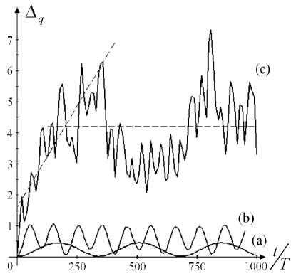
FIG. 2.: Time dependence of the variance $\Delta_{q}$ for different initial states at coupling resonance for the group with $q=0$: (a) the lowest level with $s=0$, (b) the above-separatrix level with $s=45$, (c) the near separatrix level with $s=22$. Here $a=0.01$ and $f_{0}=10$.

In Fig. 2 typical dependencies of the variance $\left(\Delta\bar{H}\right)^{2}=\omega^{2}_{n_{0}}\Delta_{q}$ of the energy are shown versus the time measured in the number $N$ of periods of the external perturbation, for different initial conditions. The quantity $\Delta_{q}$ is defined as follows,

$$\Delta_{q}=\sum_{q}(q-\bar{q})^{2}\sum_{s}|C_{q,s}|^{2},\,\,\,\,\,\,\,\,\,\bar{q}=\sum_{q}q\sum_{s}|C_{q,s}|^{2}.$$ (18)

The data clearly demonstrate a different character of the evolution of the system in dependence on the initial state. For the state taken from the center of the coupling resonance, as well as above the separatrix, the variance oscillates in time, in contrast with the state taken from inside the separatrix. In the latter case, after a short time the variance of the energy increases linearly in time, thus manifesting a diffusion-like spread of the wave packet.

In order to characterize the speed of the diffusion, we have calculated the classical diffusion coefficient $D_{cl}$ for the coupling resonance $\eta=1$, in the comparison with the quantum one, $D_{q}$, for different goffer amplitude and initial wave number $k\neq 0;\pm 1/2$, see Fig. 3. It was found that the quantum Arnol’d diffusion roughly corresponds to the classical one. However, one can see a systematic deviation which indicates that the quantum diffusion is weaker than the classical Arnol’d diffusion. This deviation is due to the influence of coherence quantum effects which can be very strong even in a deep semiclassical region. As was shown in Ref. [13], these stabilizing quantum effects are enhanced for the motion inside narrow stochastic layers surrounding the nonlinear resonances. This effect is due a relatively small number $M_{s}$ of quantum states belonging to the region of the separatrix, the fact which is crucial in the study of the quantum-classical correspondence for the systems with a weak chaos in the classical limit.

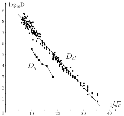
FIG. 3.: Classical $D_{cl}$ versus quantum $D_{q}$ diffusion coefficients in the dependence on the amplitude $a$ of the rippled profile.

In this connection it is instructive to estimate the number of the energy states that occupy the separatrix layer in our calculations. We have found that for $a=0.01$ of the amplitude characterizing the upper profile of the waveguide, the number of stationary states in the separatrix chaotic layer is about $M_{s}\approx 10$, therefore, one can treat our results semiclassically. Our additional calculation has shown that with the decrease of the amplitude $a$, the number $M_{s}$ decreases, and for $1/\sqrt{a}\approx 20$ this number is of the order one. For this reason the last right point in Fig. 3 corresponds to the situation when the chaotic motion along the coupling resonance is completely suppressed by quantum effects. This effect is known as the “Shuryak border” [13]) which establishes the conditions for a complete suppression of classical chaos.

Since the diffusion along the coupling resonance is effectively one-dimensional, one can expect an Anderson-like localization which is known to occur in the presence of any weak disorder in low-dimensional structures. Indeed, the variance of the QE eigenstates of the evolution operator is finite in the $q$-space. This means that eigenstates are localized, and the wave packet dynamics in this direction has to reveal the saturation of the diffusion. More specifically, one can expect that the linear increase of the variance of the energy ceases after some characteristic time.

In order to observe the dynamical localization in our model (along the coupling resonance inside the separatrix layer), one needs to analyze a long-time dynamics of wave packets. Our numerical study for large times (see curve (c) in Fig. 2) have revealed that after some time $t\sim 200T$, the diffusion-like evolution terminates for all range of the amplitude $a$. Specifically, on a large time scale the variance starts to oscillate around a mean value. This effect is of the same origin as the so-called dynamical localization which was discovered in the kicked rotor model [14, 15]. One should note that the dynamical localization is, in principle, different from the Anderson localization, since the latter occurs for the models with random potentials. In contrast, our model is the dynamical one (without any randomness), and a kind of pseudo-randomness is due to the quantum chaos mechanism.

In conclusion, we have studied the quantum Arnol’d diffusion for a particle in the quasi-1D rippled waveguide under the time-periodic electric field. This diffusion is known to occur in the corresponding classical systems, below the threshold of an overlap of nonlinear resonances resulting in a strong chaos. As is known, in this case the chaotic motion is possible only for the trajectories inside narrow stochastic layers surrounding the nonlinear resonances. The classical Arnol’d diffusion is exponentially weak, however, it leads to the unbounded motion inside the resonance web created by the resonances of different orders.

The problem under study was to find out whether the Arnol’d diffusion is feasible in quantum systems describing the electron motion in quasi-1D waveguides. Our results clearly demonstrate the peculiarities of the quantum Arnol’d diffusion and establish the conditions under which it can be observed experimentally. One of the most important results is that the quantum diffusion is typically weaker than the corresponding classical one. The analysis has shown that the reason is the influence of quantum coherent effects which are essentially strong for the motion in the vicinity of the nonlinear resonances, in the case when these resonances do not overlap. Moreover, we found that with a decrease of the perturbation responsible for the creation of stochastic layers, the quantum Arnol’d diffusion can be completely suppressed, thus leading to the absence of any chaos in the system.

Another important result is the observation of the dynamical localization of the Arnol’d diffusion, which is manifested by the termination of the diffusion on a large time scale. We have briefly discussed the mechanism of this phenomenon, relating it with the famous Anderson localization known to occur in low-dimensional disordered structures. Thus, in addition to the Shuryak border, the dynamical localization is a new mechanism destroying the quantum Arnol’d diffusion.

Recently, the weak electron diffusion was observed experimentally  [16] in superlattices with stationary electric and magnetic fields. At certain voltage, the unbounded electron motion along a stochastic web changes the conductivity of the system and results in a large increase of the current flow through the superlattice. Similarly, one can expect that electron Arnol’d diffusion inside resonance stochastic layers can increase the high frequency conductivity of a rippled channel, and can be detected experimentally.

This work was supported by the program “Development of scientific potential of high school” of Russian Ministry of Education and Science and partially by the CONACYT (México) grant No 43730. A.I.M. acknowledges the support of non-profit foundation “Dynasty”.

REFERENCES

- [1] B.V. Chirikov, Atomnaya Energia 6, 630 (1959) [Engl. Transl. J. Nucl. Energy Part C: Plasma Phys. 1, 253 (1960)].
- [2] A.J. Lichtenberg and M. A. Lieberman, Regular and Chaotic Dynamics, Springer-Verlag, New York, 1992.
- [3] V.I. Arnol’d, DAN USSR 156 (1964) 9 (in Russian).
- [4] B.V. Chirikov, Phys. Rep. 52 (1979) 263.
- [5] G.A. Luna-Acosta, A.A. Krokhin, M.A. Rodriguez, P.H. Hernandez-Tejeda, Phys. Rev. B 54 (1996) 11410.
- [6] G.A. Luna-Acosta, K. Na, L.E. Reichl, A.A. Krokhin, Phys. Rev. E 53 (1996) 3271.
- [7] G.A. Luna-Acosta, J.A. Mendez-Bermudez, F.M. Izrailev, Phys. Rev. E 64 (2001) 036206.
- [8] C.S. Lent, M. Leng, J. Appl. Phys. 70 (1991) 3157.
- [9] F.M. Izrailev, J.A. Mendez-Bermudez, and G.A. Luna-Acosta, Phys. Rev. E 68 (2003) 066201; F.M. Izrailev, N.M. Makarov, M. Rendon, arXiv:cond-mat/0411739 (2004).
- [10] L.P. Kouwenhoven et al., Phys. Rev. Lett. 65 (1990) 361.
- [11] V.Ya. Demikhovskii, F.M. Izrailev, and A.I. Malyshev, Phys. Rev. Lett. 88 (2002) 154101; V.Ya. Demikhovskii, F.M. Izrailev, and A.I. Malyshev, Phys. Rev. E 66 (2002) 036211.
- [12] V.Ya. Demikhovskii, S.Yu. Potapenko, A.M. Satanin, Fiz. Tekh. Poluprovodn. 17 (1983) 213 [Sov. Phys. Semicond. 17 (1983) 137].
- [13] E.V. Shuryak, Zh. Eksp. Teor. Fiz. 71 (1976) 2039 (in Russian).
- [14] G. Casati, B.V. Chirikov, F.M. Izrailev, and J. Ford, Lect. Notes Phys., 93 (1979) 334.
- [15] B.V. Chirikov, F.M. Izrailev, and D.L. Shepelyansky, Sov. Sci. Rev. 2 (1981) 209.
- [16] T.M. Fromhold et al., Nature 428 (2004) 726.