Calculations of time-dependent observables in non-Hermitian quantum mechanics: The problem and a possible solution

Abstract

The solutions of the time independent Schrödinger equation for non-Hermitian (NH) Hamiltonians have been extensively studied and calculated in many different fields of physics by using $L^{2}$ methods that originally have been developed for the calculations of bound states. The existing non-Hermitian formalism breaks down when dealing with wavepackets(WP). An open question is how time dependent expectation values can be calculated when the Hamiltonian is NH ? Using the F-product formalism, which was recently proposed, [J. Phys. Chem., 107, 7181 (2003)] we calculate the time dependent expectation values of different observable quantities for a simple well known study test case model Hamiltonian. We carry out a comparison between these results with those obtained from conventional(i.e., Hermitian) quantum mechanics (QM) calculations. The remarkable agreement between these results emphasizes the fact that in the NH-QM, unlike standard QM, there is no need to split the entire space into two regions; i.e., the interaction region and its surrounding. Our results open a door for new type of WP propagation calculations within the NH-QM formalism that until now were impossible. In particular our work is relevant to the many different fields in physics and chemistry where complex absorbing potentials are introduced in order to reduce the propagation calculations into a restricted region in space where the artificial reflections from the edge of the numerical grid/box are avoided.

1 Introduction

In the last two decades there has been an increasing interest in non-Hermitian(NH) quantum mechanics (QM) in many different fields of physics. In many studied cases in atomic, molecular and nuclear physics the Hamiltonian is NH due to the use of different type of analytical continuation transformations. One such method is complex scaling (CS) where $\hat{H}({\bf r})\to\hat{H}({\bf r}e^{\imath\theta})$ [1][2][3][4]. Another common method is the introduction of complex absorbing local energy independent potentials (CAPs), also known as optical potentials, into the Hamiltonian[5][6] such that $\hat{H}\to\hat{H}+\hat{V}_{CAP}$. The complex eigenvalues and eigenfunctions of the NH Hamiltonians, in these studies, were calculated using square-integrable methods that were originally developed for the calculation of bound states (see references to reviews mentioned above). The need to replace the scalar product which is used in conventional QM by a generalized inner product is well understood and has been discussed quite extensively in the literature. See for example the different approaches for generalized inner products in NH-QM in Ref. [7] and Ref.[8] and references therein. However, for the sake of clarity in Section 2.1 we provide a brief account of the generalized inner product (so called c-product[9]) which has been used until now for calculating time independent observables in NH-QM[4]. It is quite straightforward to apply the same generalized definition of the inner product to NH time periodic Hamiltonians ( see for example Ref.[4]), which describe the interaction of atoms or molecules with oscillating electric field. The application of the NH formalism to laser driven system has been very useful in explaining physical phenomena. For example, remarkable agreement has been achieved between the results obtained from theoretical NH-QM calculations and the experimental results of the probability of generating odd high-order harmonics (i.e., generation of high energy photons resulting from the absorbtion of many low energy photons)[10]. However, one important problem remains open. How to calculate the entire high-order harmonic generation spectra and not only the probabilities to obtain even or odd harmonics ? This question is related to a more general question. How to calculate time dependent expectation values in NH-QM ? In NH-QM the propagated right wavepacket (WP) is the solution of the time dependent Schrödinger equation (TDSE) where $\hat{H}$ is a NH Hamiltonian.

$$\hat{H}\Psi({\bf r},t)=\imath\hbar\frac{\partial}{\partial t}\Psi({\bf r},t)\quad.$$ (1)

Extensive WP propagation calculations were carried out for complex potential energy surfaces by solving the NH-TDSE (see for example Refs.[11, 12, 13, 14, 15]). However, in order to calculate time dependent expectation values one needs to carry out WP propagation calculations from $t=0$ to $t=-\infty$. The problem is that in NH-QM it is impossible to propagate the initial WP from t=0 to $t=-\infty$. We briefly review this known problem in Section 2.2 and relate it to the concept of time asymmetry in QM which is a subject of numerous studies in the literature (see Refs.[16, 17, 18, 19] and references therein).
Very recently a possible solution to the time asymmetry problem in NH-QM was proposed by Moiseyev and Lein[20]. The solution requires modification of the currently used inner product. As we will show in Section 3 this modification of the well known generalized inner product (briefly reviewed in Section 2.1) which we will term ”F-product” (FP) is applicable for cases where the Hamiltonian is either a time-independent or time dependent NH operator. Naturally this modification of the generalized inner product reduces to the conventional scalar product when the Hamiltonian is Hermitian. Moiseyev and Lein [20] have shown that using the modified generalized definition of the inner product not only solves the time asymmetry problem in NH-QM , but also has a very important physical implications. They have shown that the analytical expression for the high-order harmonic generation spectra (HHGS) which has been derived within the framework of the FP modified NH time dependent formalism, clearly indicates why only odd high-order harmonics were observed in experiments where high-intensity laser pulses have been used. Moreover, the analysis of the expressions they obtained for the HHGS indicates under what conditions also even high-order harmonics would be observed. Simulation calculations within the framework of the conventional (hermitian) QM based on their finding supported their results. The possibility of generating also the even-order harmonics as well as the odd ones should help in generating ultra short high intensity laser pulses. However, so far the FP generalized inner product as first proposed in ref[20] has never been tested for numerical NH calculations. The purpose of this work is to calculate time-dependent observable quantities for a well known test case study problem within the framework of the FP formalism and compare it with the results obtained from the conventional (i.e., Hermitian) QM. As we will show here such a comparison clearly shows that time dependent observables should be calculated within the framework of the FP formalism and also give some physical interpretation of this formalism.

2 Non-Hermitian Hamiltonians, and their consequence

Non-Hermitian Hamiltonians have been used to describe a variety of physical phenomena. The methods by which the Hamiltonian becomes NH are also diverse. Such methods include for example the addition of complex absorbing potentials to the Hamiltonian or the scaling of the coordinate by a complex factor. The use of NH Hamiltonians results in complex eigenvalues,

$$E_{\alpha}=\varepsilon_{\alpha}-\imath\Gamma_{\alpha}/2\quad,$$ (2)

where often the real part, $\varepsilon_{\alpha}=\textit{Re}(E_{\alpha}$), is associated with the energy while the complex part is related to the decay rate, $\Gamma_{\alpha}$ of a metastable state by: $\Gamma_{\alpha}=-2{\textit{Im}}(E_{\alpha})$ such that the lifetime of the metastable state is given by $\hbar/\Gamma_{\alpha}$. When using NH Hamiltonians one needs to address the aspects that differ from conventional QM.

2.1 Brief account of the generalized inner product: the c-product

As a result of the NH nature of the Hamiltonian, there is a need to define a generalized inner product. The question of the definition of the inner product when the Hamiltonian is NH is a crucial one, especially in time dependent calculations. Let us consider a general case where the Hamiltonian, $\hat{H}$ can be either Hermitian or NH Hamiltonian. Since the concept of a generalized inner product is well defined in linear algebra for general not necessarily Hermitian matrices[21] we begin our brief review by the representation of the Hamiltonian by a matrix $\bf H$. The Hamiltonian matrix elements are defined as

$$H_{i,j}=<\varphi_{i}|{\hat{H}}|\varphi_{j}>$$ (3)

where $\{\varphi_{i}\}$ are orthonormal square integrable basis set functions in the Hilbert space. We assume here that we can truncate the number of the basis functions and represent the Hamiltonian by a finite general complex matrix. The matrix can be as large as one wishes. The matrix $\bf H$ has right and left eigenvectors. Let us denote the right (column) eigenvectors by ${\vec{\Phi}}_{\alpha}^{R}$ and the left (row) eigenvectors by $({\vec{\Phi}}_{\alpha^{\prime}}^{L})^{t}$. That is,

$${\bf H}{\vec{\Phi}}_{\alpha}^{R}=E_{\alpha}{\vec{\Phi}}_{\alpha}^{R}$$ (4)

and

$$({\vec{\Phi}}_{\alpha^{\prime}}^{L})^{t}{\bf H}=E_{\alpha^{\prime}}({\vec{\Phi}}_{\alpha^{\prime}}^{L})^{t}$$ (5)

By taking the transpose of Eq.5 one gets,

$${\bf H}^{t}{\vec{\Phi}}_{\alpha^{\prime}}^{L}=E_{\alpha^{\prime}}{\vec{\Phi}}_{\alpha^{\prime}}^{L}$$ (6)

The matrix $\bf H$ and its transpose ${\bf H}^{t}$ support the same spectrum. We define the generalized inner product, termed c-product [9], such that for non degenerate states where $E_{\alpha^{\prime}}\neq E_{\alpha}$,

$$({\vec{\Phi}}_{\alpha^{\prime}}|{\vec{\Phi}}_{\alpha})\equiv({\vec{\Phi}}_{\alpha^{\prime}}^{L})^{t}\cdot{\vec{\Phi}}_{\alpha}^{R}=0$$ (7)

From Eq.6 it is obvious that when $\bf H$ is Hermitian matrix (i.e., ${\bf H}^{t}={\bf H}^{*}$) then ${\vec{\Phi}}_{\alpha^{\prime}}^{L}=({\vec{\Phi}}_{\alpha^{\prime}}^{R})^{*}$ and the c-product $(...|...)$ is equal to the known scalar product $<...|...>$. If for example $\bf H$ is a symmetric matrix (note any matrix can be transformed to a symmetric form and therefore a complex symmetric matrix is a general representation of a NH matrix) then,

$${\vec{\Phi}}_{\alpha}^{L}={\vec{\Phi}}_{\alpha}^{R}$$ (8)

Do the eigenvectors of a non-hermitian matrix $\bf H$ form a complete set ? A complete set implies that the number of linearly independent eigenvectors is equal to the dimension of the matrix. It may happen that due to a coalescence of two eigenvectors (coalescence of more than two eigenvectors is very unlikely phenomena[21][22]) the number of the linearly independent eigenvectors is smaller than the dimension of the matrix and the spectrum is incomplete. This coalescence of the eigenvalues happens at $\alpha=\alpha_{b}$ (where ”b” stands for a branch point in the complex energy plane[22])for $\alpha\to\alpha_{b}$ the specific eigenvector denoted by $\alpha=\alpha_{b}$ is ”self-orthogonal” in the sense that, $({\vec{\Phi}}_{\alpha_{b}}|{\vec{\Phi}}_{\alpha_{b}})=0$. However, due to round off numerical errors it is quite impossible to get the incomplete spectrum and always in the numerical calculations the eigenvectors are normalizable such that. $({\vec{\Phi}}_{\alpha}|{\vec{\Phi}}_{\alpha})=1$ [23]. As the number of the basis functions, $\{\varphi_{i}\}$, which are used to construct the Hamiltonian matrix in Eq.3)is increased, the function $\Phi_{\alpha}^{R}(N)$ given by:

$$\Phi_{\alpha}^{R}(N)=\sum_{i=1}^{N}[{\vec{\Phi}}_{\alpha}^{R}]_{i}\varphi_{i}$$ (9)

gives a better description of the $\alpha-th$ eigenfunction of the Hamiltonian. It is out of the scope of this paper to describe the complex (i.e., NH) variational theorem that has been proved for complex symmetric Hamiltonian matrices (see Ref.[4] and references therein). However, on the basis of the complex variational principle the exact eigenfunction, $\phi_{\alpha}^{R}$ can be expressed as,

$$\phi_{\alpha}^{R}=\lim_{N\to\infty}\Phi_{\alpha}^{R}(N)$$ (10)

and similarly,

$$\phi_{\alpha}^{L}=\lim_{N\to\infty}\Phi_{\alpha}^{L}(N)=\lim_{N\to\infty}\sum_{i=1}^{N}[{\vec{\Phi}}_{\alpha}^{L}]_{i}\varphi_{i}^{*}$$ (11)

where,

$${\hat{H}}\phi_{\alpha}^{R}=E_{\alpha}\phi_{\alpha}^{R}$$ (12)

and

$${\hat{H}}^{\dagger}\phi_{\alpha}^{L*}=E_{\alpha}^{*}\phi_{\alpha}^{L*}$$ (13)

Here ${\hat{H}}^{\dagger}$ is the hermitian conjugate of $\hat{H}$ such that,

$$<\varphi_{i}|{\hat{H}}^{\dagger}|\varphi_{j}>=[<\varphi_{j}|{\hat{H}}|\varphi_{i}>]^{*}$$ (14)

The basis functions are square integrable functions as described above. Now, the generalized inner product (so called c-product) for the left and right eigenfunction, $\{\phi_{\alpha}^{L},\phi_{\alpha}^{R}\}$, will be defined by:

$$(\phi_{\alpha^{\prime}}|\phi_{\alpha})\equiv\int_{all-space}\phi_{\alpha^{\prime}}^{L}\phi_{\alpha}^{R}dv=\delta_{\alpha^{\prime},\alpha}$$ (15)

Note that the c-product, $(\phi_{\alpha}|\phi_{\alpha})$, may be complex and may have negative real or imaginary parts, therefore the c-product is not a metric scalar product [9]. For a physical interpretation of the complex density probability $\phi_{\alpha}^{L}\phi_{\alpha}^{R}$ see Ref.[24].

2.2 Brief account of the time asymmetry problem in NH-QM

Time asymmetry in physics is a concept closely related to irreversibility which has been a subject of many theoretical studies. The conventional Hermitian QM is time-symmetric in the sense that it is described by an equation symmetrical with respect to time and by time-symmetric boundary conditions[16]. The process of the decay of a metastable state is an irreversible one in the sense that it can only be described from a certain time $t=0$ to time $t=\infty$. Authors such as Bohm [16], Prigogine [17], Sudarshan et. al. [18] have constructed formalisms which incorporate the irreversible nature of the resonance phenomena into QM usually by relying on the introduction of rigged Hilbert spaces. This leads to semi group evolution which distinguished between ”prepared” stated and ”measured” states [16]. However, it has been argued by Nicolaides [19] that time asymmetry results from complex energy distribution without the need to introduce rigged Hilbert spaces.
Indeed, in the spirit of Ref.[19], we will show that in NH-QM, within the spectral representation of the NH Hamiltonian, time asymmetry will pose a problem in the propagation of WP’s. The need to carry out WP calculations within the framework of NH-QM is a crucial point in the study of systems where the dynamics are not controlled by a single resonance state. When one tries to propagate a WP in NH-QM the evolution of each of the stationary eigenfunctions in Eq.12 is governed by the NH-TDSE and the stationary solutions of Eq.1 are given by:

$$\psi_{\alpha}^{R}(t)=\exp(-\imath E_{\alpha}t/\hbar)\phi_{\alpha}^{R}\quad.$$ (16)

When one attempts to propagate the corresponding stationary solutions of the transposed NH Hamiltonian $\hat{H}^{t}=\hat{H}^{{\dagger}*}$ (see Eq.13), at time $t$ the left eigenfunctions will be given by:

$$\psi^{L}_{\alpha}(t)=\exp(+iE_{\alpha}t/\hbar)\phi_{\alpha}^{L}\quad.$$ (17)

Since $E_{\alpha}={\cal E}_{\alpha}-\imath\Gamma_{\alpha}/2$ the left eigenfunctions diverge exponentially as $t\rightarrow\infty$. In Hermitian QM $\psi^{L}_{\alpha}=\psi^{*}_{\alpha}$ and $E_{\alpha}$ is real, thus, $\psi^{L}_{\alpha}$ does not diverge. Since the only difference from the evolution of $\psi^{R}_{\alpha}$ is in the $+$ sign in the exponent it is similar in a way to propagating the initial state to a negative time. Since in NH-QM the energy is complex, the wavefunction cannot be propagated backward to $-\infty$ but only forward to $+\infty$. This time asymmetry problem dissolves when studying cases where only one metastable state dominates since when calculating any observable quantity the time dependent phases of the right and left eigenfunctions, $\exp(\pm\imath E_{\alpha}t/\hbar)$, cancel out. When one studies the evolution of a WP, the right function obeys the NH-TDSE in Eq.1 and can be constructed as a linear combination of the eigenfunctions of the NH Hamiltonian given in Eq.16. The left function will be a linear combination of the eigenfunctions given in Eq.17. Now, when calculating any observable quantity, which does not commute with $\hat{H}$, there will be cross terms between different eigenfunctions with time dependent phase of the form, $\exp(\imath(E_{\alpha}-E_{\alpha^{\prime}})t/\hbar)$. These terms will diverge at long times as $\exp((\Gamma_{\alpha}-\Gamma_{\alpha^{\prime}})t/2)$ and prevent the calculation of observable quantities of a WP in NH-QM.
This is, in short, the time asymmetry problem in NH-QM. Due to this problem the calculation of observables in NH-QM is feasible only when one long lived metastable state controls the dynamics of the system and $\psi_{\alpha}^{L}(t)\psi_{\alpha}^{R}(t)=\phi_{\alpha}^{L}\phi_{\alpha}^{R}$ is time independent. A definition of an observable for a general superposition of resonance states is required. This subject will be discussed in Sections 3 and 4.

3 Wavepacket propagation in the F-Product formalism

As stated earlier the time asymmetry problem prevents the propagation of WP’s backward in time in NH-QM. The existing definition of the left eigenfunctions of the NH Hamiltonian is based on the c-product as defined in section 2.1 by Eq.17, which diverges exponentially in time due to the complex part of the energy. The one-state probability density $\psi_{\alpha}^{L}\psi_{\alpha}^{R}=\phi_{\alpha}^{L}\phi_{\alpha}^{R}$ is complex and time independent. However, as mentioned before the imaginary part of the complex energy is associated with the decay of a metastable state therefore one would expect that the probability to find the particle in such a state should decay in time with a rate of decay $\Gamma_{\alpha}$.
In order to impose this decay behavior of a metstable state we apply the finite-range F-product (FP) formalism which was proposed in Ref.[20] but was never tested by carrying out WP propagation calculations within the framework of NH-QM. For the sake of clarity let us first explain the idea behind the F-product formalism. As we have seen in section 2.2, when the left function is stationary solution of Eq. 13 it is defined by Eq.17. Although $\psi_{\alpha}^{L}(t)$ diverges exponentially as time goes to infinity, the norm is preserved and $(\psi_{\alpha}(t)|\psi_{\alpha}(t))=(\phi_{\alpha}|\phi_{\alpha})=1$. This result is due to the fact that we integrate over the entire space and the probability to find the particle somewhere in space is unity. In order for the probability density to decay with time we need to divide the entire space into two parts. One part is the interaction region which we associate with our system that in time breaks up into sub-systems. The complimentary part is defined as a ”surrounding” or as the ”environment” of our system. We require from an isolated single metastable state to decay exponentially (a first order ’reaction’) n time as the sub-systems escape from the interaction region to the ”environment”.
An acceptable way to separate the ”system” from the ”surrounding” is by the well known Feshbach formalism [25], which is often used for describing systems in nuclear physics. Here the Hamiltonian is split by two operators $Q$ and $P$ which project the system into subspaces of discrete and continuum states respectively. The resulting Hamiltonian for the bound part of the system is given by:

$$\hat{H}_{FF}=\hat{H}_{QQ}+V_{QP}\hat{G}_{P}^{+}V_{PQ}\quad,$$ (18)

where, $\hat{H}_{QQ}$ is the Hamiltonian for the ”system” and $\hat{G}_{P}^{+}=\lim_{\epsilon\to 0^{+}}(E-\hat{H}_{PP}+i\epsilon)^{-1}$ is the Green operator for the particle in the continuous or dissociative part of the spectrum which describes the ”surrounding” to which the particles decay. The effective Hamiltonian as defined in Eq. 18 is a NH operator. It is clear that here the effective Hamiltonian is NH due to splitting of space into an interaction region where our system is located and a ”surrounding” which absorbs the emitted particles (sub-systems). However, we wish to associate the decay phenomena with particles which ”escape” from the interaction region to its ”surrounding” even in cases where the NH formalism takes the entire space into account. How to split the entire space in the most general case into an interaction region and its ”surrounding” ? We will return to this question in the next section. Here we argue that when the dynamics is controlled by a single isolated metastable state within the NH-QM formalism then we may use the finite box quantization approach where the interaction region can be defined as a box as large as one wishes. In such a case the integrals are calculated not over the entire space, i.e., from $-\infty$ to $+\infty$, but from $-a/2$ to $+a/2$ where the size of the box, $a$, is as large as one wishes, hence the name - finite-range given to this new formalism. Since we want to describe a decay phenomena we now define the evolution of the left eigenfunctions as,

$$\psi_{\alpha}^{L}=\exp(\imath E_{\alpha}^{*}t/\hbar)\phi_{\alpha}^{L}=\exp(\imath\varepsilon_{\alpha}t/\hbar)\exp(-\Gamma_{\alpha}t/(2\hbar))\phi_{\alpha}^{L}\quad.$$ (19)

Now the probability do detect the particle in a decaying state will decrease exponentially in time according to:

$$(\psi_{\alpha}|\psi_{\alpha})=\exp(-\Gamma_{\alpha}t/\hbar)(\phi_{\alpha}|\phi_{\alpha})=\exp(-\Gamma_{\alpha}t/\hbar)\quad.$$ (20)

This definition also prevents the divergence in time of the left functions and enables the propagation of a WP in time. Within the FP formalism a WP will be now defined by a superposition of the eigenfunctions of the NH Hamiltonian.

$$\Psi^{R}_{FP}=\sum_{\alpha}C_{\alpha}^{R}\exp(-\imath E_{\alpha}t/\hbar)\phi_{\alpha}^{R}\qquad;\qquad\Psi^{L}_{FP}=\sum_{\alpha}C_{\alpha}^{L}\exp(\imath E_{\alpha}^{*}t/\hbar)\phi_{\alpha}^{L}\quad,$$ (21)

where

$$C_{\alpha}^{R}=\left(\phi_{\alpha}|\Psi_{FP}(t=0)\right)\qquad;\qquad C_{\alpha}^{L}=\left(\Psi_{FP}(t=0)|\phi_{\alpha}\right)\quad.$$ (22)

When the Hamiltonian is NH due to the application of one of the complex scaling (CS) similarity transformations, then the initial state $\Psi_{FP}(t=0)$ is given by ${\hat{S}}\Psi(t=0)$ where $\hat{S}$ is one of the CS transformations[26]. On the other hand when CAP is added to the Hamiltonian and the initial state is localized in the interaction region it remains unscaled. An important point in the new definition of the inner product is that now the right-WP satisfies the NH-TDSE as defined in Eq.1, whereas the left-WP does not satisfy a corresponding wave equation. This is a very important point in our search for solution of the time asymmetric problem in NH-QM. The FP definition of the inner product generalizes only the time dependence of the c-product definition. Therefore, when the functions are time independent the F-product reduces to the c-product. Based on the Eq. 21 the decay of a WP will now be given by:

$$\left(\Psi_{FP}|\Psi_{FP}\right)=\sum_{\alpha}C_{\alpha}^{L}C_{\alpha}^{R}\exp\left(-\Gamma_{\alpha}t/\hbar\right).$$ (23)

Note that although there are no cross terms between different $\alpha$’s there are still interference effects since $C_{\alpha}^{L}C_{\alpha}^{R}$ have complex values. Nevertheless the absolute value of this expression decays continuously as time passes. The goal of this paper is to check the FP formalism for the first time for a simple test model problem and compare the results with those obtained from conventional QM calculations. Such a comparison is made in section 4.

4 Application to a simple one dimensional problem

We would like to implement the new formalism on a simple one dimensional time independent Hamiltonian, which will serve as a test model:

$$\hat{H}(x)=\frac{\hat{p}^{2}}{2m}+(\frac{x^{2}}{2}-0.8)\exp(-0.1x^{2})\quad,$$ (24)

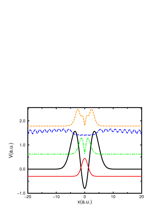
Figure 1: (Color Online) Eigenfunctions of the model potential in Eq.25. The solid line is for the bound state; the dot-dashed line is for an isolated resonance; The long dashed line is for a continuum state just under the top of the barrier; and the dashed line is for a broad resonance over the barrier.

This model Hamiltonian has been often used as a test case for new theories and computational methods(see for example [27]). The potential in Eq.24 consists of a potential between two barriers (See Fig.1). In the example presented below the Hamiltonian becomes NH upon complex scaling of the coordinate by a complex phase, $\theta$, such that $x\to x\exp(\imath\theta)$ and is given by:

$$\hat{H}_{\theta}(x)=e^{-2\imath\theta}\frac{\hat{p}^{2}}{2m}+(\frac{e^{2\imath\theta}x^{2}}{2}-0.8)\exp(-0.1e^{2\imath\theta}x^{2})\quad,$$ (25)

The model potential shown in Fig.1 supports a bound state and two metastable resonances below the top of the barrier as well as several other resonances over the barrier. The resonances are localized states that decay in time and cannot be described by a single eigenfunction of the Hermitian Hamiltonian in Eq.24, however in NH-QM they are represented by a single square integrable eigenfunction of the NH Hamiltonian in Eq.25 as can be seen in Fig.1. Our objective is to show that the FP formalism will yield similar results to those obtained by conventional Hermitian QM, without the need to divide our space to ”system” and ”surrounding”. For this purpose lets define now the interaction region as the area between the top off the two barriers in Fig.1 and return to this point later on.
In order to observe the decay of a WP with time we will place a gaussian WP in the center of the potential in Eq.24 of the form:

$$\Psi(0)=\frac{1}{(\pi\sigma^{2})^{1/4}}\exp\left(-\frac{x^{2}}{2\sigma^{2}}+\imath k_{0}x\right)\quad,$$ (26)

where $\sigma$ is the width of the WP and $k_{0}$ its initial momentum. Upon CS the right initial state WP becomes:

$$\Psi^{R}(0)=\frac{e^{\imath\theta}}{(\pi\sigma^{2})^{1/4}}\exp\left(-\frac{e^{2\imath\theta}x^{2}}{2\sigma^{2}}+\imath e^{\imath\theta}k_{0}x\right)\quad,$$ (27)

while the left initial WP is given by:

$$\Psi^{L}(0)=\frac{e^{\imath\theta}}{(\pi\sigma^{2})^{1/4}}\exp\left(-\frac{e^{2\imath\theta}x^{2}}{2\sigma^{2}}-\imath e^{\imath\theta}k_{0}x\right)\quad.$$ (28)

Note that at time $t=0$ the definitions of the c-product and the F-product are identical and $\left(\Psi^{L}(0)|\Psi^{R}(0)\right)=1$. The norm of the WP, ${\cal N}_{FP}(t)$, within the FP formalism, as defined in Eq.21, and is given by:

$${\cal N}_{FP}(t)=\int_{\infty}^{\infty}\Psi^{L}_{FP}(x,t)\Psi^{R}_{FP}(x,t)dx=\sum_{\alpha}C_{\alpha}^{L}C_{\alpha}^{R}\exp(-\Gamma_{\alpha}t/\hbar)\quad.$$ (29)

Assuming the decay of the WP is a first order process the effective decay rate will be given by:

$$k_{FP}(t)=-\frac{d}{dt}\ln{\cal N}_{FP}(t)\quad.$$ (30)

When the WP populates several resonance states the effective decay rate will be time dependent, but when only one resonance state is populated the anticipated constant effective decay rate will be obtained, $k_{FP}=\Gamma_{res}/\hbar$. In contrast, the decay will not be observed in Hermitian QM where the norm is conserved. Therefore we choose a new quantity for comparison with the norm in Eq.29, which we will label ${\cal N}_{QM}$ and is defined by the part of the WP which is localized inside the interaction region.

$${\cal N}_{QM}(t)=\int_{-a/2}^{a/2}\Psi^{*}_{QM}(x,t)\Psi_{QM}(x,t)dx\quad,$$ (31)

where $\Psi_{QM}(x,t)$ is the result obtained from conventional propagation calculations, when by conventional we mean the solution of the Hermitian TDSE. This enables us to define an effective decay rate even in Hermitian QM based on Eq.31.

$$k_{QM}(t)=-\frac{d}{dt}\ln{\cal N}_{QM}(t)\quad.$$ (32)

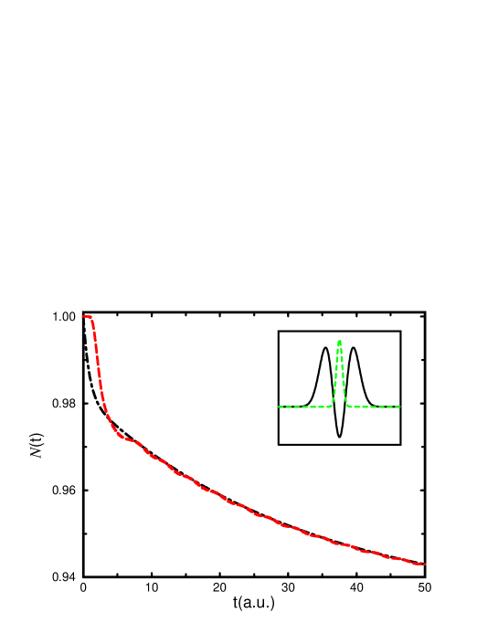
Figure 3: (Color Online) The same as Fig2, but with an initial state of a narrow gaussian, $\sigma=0.71a.u.$, fully localized in the interaction region around $x=0$ (shown in the inset). The dot-dashed line is for Eq.29 and the long dashed line for Eq.31.

The question we address ourselves with now is how to define the interaction region ? or similarly what is $a$ in Eq.31 ? Is the initial assumption that we can define the interaction region as the area between the top of the two barriers valid? Here, we are not using the Feshbach formalism and therefore we look for a simple universal definition. We propose here to define the interaction region (the parameter ”a” in our 1D case or the vector $\vec{a}$ in multidimensional case) based on the NH calculations. More precisely we wish to define the interaction region as the region where the resonances are localized. The continuum states in the same energy range have a very small (almost vanishing ) amplitude in this region as can be seen in Fig.1. This definition is obviously not an exact one and its important to note that using the FP formalism we avoid the need to define the interaction region and thus $a$ is only relevant when trying to relate the results to conventional QM. The results which will be presented below strongly support our conjecture.
Returning to the problem of the decay of the norm of a WP, we first place a gaussian WP as shown in Eq.26 with $\sigma=3.87a.u.$ and $k_{0}=0$. It is evident on Fig.2 that on the long time scale there is a remarkable correspondence between the results of Eq.29 and Eq.31. On short times there is deviation which results from the fact that the decay of the resonances starts at time $t=0$ whereas for an Hermitian WP it will take time to reach the boundary of the interaction region. The idea is simple. Using the NH F-product formalism the resonance states decay at any time including the extremely short time regime. In conventional propagation calculations the initial WP oscillates in between the barriers and a significant part of the tunnelling takes place when the oscillating WP hits the inner classical turning points of the potential barriers. Therefore the deviation between the results obtained from NH-QM and conventional QM calculations is during the time it takes for the initial WP to reach the inner classical turning points. To further illustrate this if we study a narrow WP with $\sigma=0.71a.u.$, which is fully localized between the barriers inside the potential in Fig. 1 it is obvious from the above argument that in Hermitian QM it will take the WP some time to escape out of the barriers while in NH-QM decay starts immediately at $t=0$ (see Fig3). When one studies the behavior of different WP’s, the best choice for $a$ in Eq.31 varies and depends on the WP but it is always in the vicinity of the top of the barriers in Fig.1. This can be understood again by realizing that the continuum wavefunctions under the top of the barrier are localized outside of the potential while the resonance states are localized inside the potential (even over the barrier), therefore, in NH-QM we have a clear distinction between the ”system” and its ”surrounding”.
In previous nuclear physics studies of the decay of narrow isolated resonances which are associated with the NH effective Hamiltonian given in Eq.18 the decay law has been obtained by the conventional scalar product [28]. Namely, following this approach the effective decay rate is given by:

$$k_{eff}(t)=-\frac{d}{dt}ln\left<\Psi^{R}(t)|\Psi^{R}(t)\right>\quad,$$ (33)

where $\Psi^{R}(t)$ is the solution of Eq.1 which can be expanded in the basis set of the eigenfunctions of Eq.12, $\{\phi^{R}_{\alpha}\}$ (with corresponding eigenvalues $E_{\alpha}$), such that $\Psi^{R}(t)=\sum_{\alpha}C_{\alpha}^{R}\phi^{R}_{\alpha}$. Using this approach one gets that,

$${\cal N}_{NP}=\left<\Psi^{R}(t)|\Psi^{R}(t)\right>=\sum_{\alpha,\alpha^{\prime}}(C_{\alpha^{\prime}}^{R})^{*}C_{\alpha}^{R}\exp[-\imath(E_{\alpha}-E_{\alpha^{\prime}})t/\hbar]\left<\phi^{R}_{\alpha^{\prime}}|\phi^{R}_{\alpha}\right>\quad,$$ (34)

where the notation $NP$ stands for the formalism used in nuclear physics in Ref.[28]. When the resonances are not isolated there is a deviation from the effective decay rate due to interference between the different states. When trying to apply this approach to our simple test model, one fails to get converged results and moreover the behavior of ${\cal N}_{NP}$ based on Eq.34, as can be seen in Fig.2, is quite irregular as it oscillates instead of constantly decaying. This shows that the formalism depicted in Eq.34 can only be used in specific cases whereas the FP formalism as portrayed in Eq. 29 should be used in general.
Let us now test the FP formalism for calculating time dependent expectations values for NH Hamiltonians. If one wishes to measure an observable quantity $\bar{A}$ which will be defined in NH-QM, within the FP formalism, by:

$$\bar{A}(t)=\frac{\left(\Psi_{FP}(t)\left|\hat{\tilde{A}}\right|\Psi_{FP}(t)\right)}{\left(\Psi_{FP}(t)|\Psi_{FP}(t)\right)}=\frac{\int_{-\infty}^{\infty}\Psi^{L}_{FP}(x,t)\hat{\tilde{A}}\Psi_{FP}^{R}(x,t)dx}{\int_{-\infty}^{\infty}\Psi_{FP}^{L}(x,t)\Psi_{FP}^{R}(x,t)dx}\quad,$$ (35)

where in principle $\bar{A}$ can get complex values. In such a case the phase of $\bar{A}$ should be a measurable quantity (and therefore should be $\theta$ independent although both $\Psi^{R}_{FP}(t)$ and $\Psi^{L}_{FP}(t)$ vary with $\theta$ (the rotational angle associated with the CS transformation). In our case (i.e., the Hamiltonian is NH due to the CS similarity transformation.) $\hat{\tilde{A}}=\hat{S}\hat{A}\hat{S}^{-1}$ is the scaled operator for the desired observable. As we have seen in Fig’s 2,3 the NH formalism describes the part of the WP which remains in the interaction region. Thus, we expect to find correspondence to a quantity similar to that defined in Eq.31. We will label $<A>$ as an observable quantity in the interaction region calculated by the conventional (Hermitian) quantum-mechanics approach.

$$<A(t)>=\frac{\int_{-a/2}^{a/2}\Psi^{*}(x,t)\hat{A}\Psi(x,t)dx}{\int_{-a/2}^{a/2}\Psi^{*}(x,t)\Psi(x,t)dx}\quad,$$ (36)

where $\Psi(x,t)$ is the solution obtained by solving the conventional TDSE. Returning to our one-dimensional test model, the results for the observable $\hat{A}=x$ of the average position for a WP placed at $x=0$ with width, $\sigma=3.87a.u.$, and initial momentum $k=1a.u.$ based on Eq.’s 35,36 are given in Fig.4. Once again there is very good correspondence on the long time scale while on the short time scale there are deviations. This suggests that the NH formalism which describes the resonance states applies on times longer than some initial rearrangement time in which the resonance states are populated.
Since the scaling parameter is not associated with any physical quantity, time dependent observables should get real values in spite of the analytical continuation of the Hamiltonian. Indeed, the results presented in Fig.5 show very clearly that at any given time the mean position, $\bar{x}(t)$,($\hat{A}=\hat{x}$ in Eq.35), and mean momentum $\bar{p}(t)$,($\hat{A}=\hat{p}_{x}$ in Eq.35) are real quantities even though they have been obtained by NH calculation based on Eq.35. The phase of both the average position and momentum is zero with abrupt shifts in $\pi$ every time an observable vanishes (and thus can’t be measured at that given time). The jumps in $\pi$ of the phase of $\bar{A}$ ($\bar{x}(t)$ or $\bar{p}(t)$) result from the fact that the observable changes its sign from positive to negative or vise-versa and therefore would appear also in standard QM calculations.

5 Conclusions

We have shown that using the recently introduced FP formalism it is possible to overcome the time-asymmetry problem in NH-QM and to propagate a WP which populates many resonance states. This formalism describes the dynamics without the need to separate the entire space into ”system” and ”surrounding” which is necessary when using Hermitian QM. The NH description of the system is valid on the timescales which are long enough to regard only the localized part of the WP after the scattered part of the WP has left the interaction region. It has also been shown that observables such as position and momentum in the F-product formalism obtain real values despite the NH nature of the Hamiltonian. This reasserts the validity of this formalism which makes it applicable to systems where particles are temporarily trapped in the interaction region. The application of these novel approach to many electron systems is under current study.

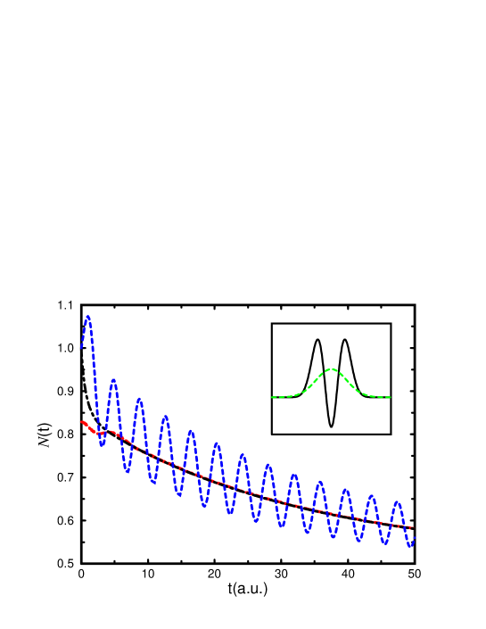
Figure 2: (Color Online) The norm of wide Gaussian WP based on the F-product formalism as given by Eq.29 (dot-dashed line)as a function of time in comparison with the part of the Hermitian WP localized inside the interaction region (long-dashed line)as given in Eq.31. The dashed line shows the norm in the formalism portrayed in Eq.34. In the inset the initial gaussian WP with width of $\sigma=3.87a.u.$ and $k_{0}=0a.u.$ .

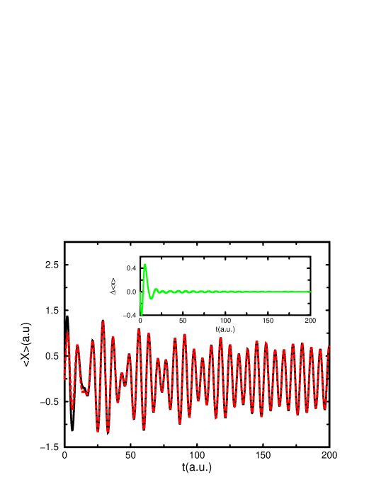
Figure 4: (Color Online) The average position of a gaussian WP with initial momentum of $k=1a.u.$ and $\sigma=3.87a.u.$ as a function of time. The solid line is for the solution in the F-product formalism as given in Eq.35while the dashed line is for the Hermitian part of the WP localized inside the interaction region as depicted in Eq.36. The inset shows the difference between the two as a function of time.

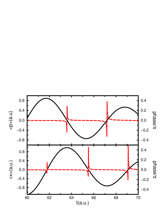
Figure 5: (Color Online) The average position (bottom) and momentum (top) of a gaussian WP with initial momentum $k=1$ in the F-Product formalism and their corresponding phases based on Eq.35. The solid line is for the real part of the average position/momentum while their corresponding phases are given by the long-dashed lines. The interval of time on which these results appear was chosen arbitrarily in order to have clear presentation, but the overall behavior is similar in all range of time. Due to the abruptness of the change the shifts in pahsesd are not exactly of $\pi$ strictly for numerical reasons.

References

- [1] B. R. Junker, Adv. At. Mol. Phys., 18, 107 (1982).
- [2] W. P. Reinhardt, Annu. Rev. Phys. Chem.,33, 223 (1982).
- [3] Y. K. Ho, Phys. Rep. C, 99, 1 (1983).
- [4] N. Moiseyev, Phys. Rep. 302, 211 (1998).
- [5] J. G. Muga, J. P. Palao, B. Navarro, and I. L. Equsquiza, Phys. Report 395, 357 (2004).
- [6] R. Santra and L. S. Cederbaum, Phys. Rep., 368, 1 (2002).
- [7] A. M. Perelomov and Ia. B. Zeĺdovich, Quantum Mechanics: Selected Topics, (World Scientific Publishing, Singapore, 1998).
- [8] E. Brändas and N. Elander (Editors), The Letropet Symposium View on Generalized Inner Product, Lecture Notes in Physics vol. 325 (Springer, Berlin, 1989).
- [9] N. Moiseyev, P. R. Certain, and F. Weinhold, Mol. Phys., 36, 1617 (1978).
- [10] N. Moiseyev and F. Weinhold, Phys. Rev. Lett., 78, 2100 (1997).
- [11] R. Kosloff and D. Kosloff, J. Comp. Phys., 63, 363 (1986); G. Ashkenazi, R. Kosloff, S. Ruhman, and H. Tal-Ezer, J. Chem. Phys, 103, 10005 (1995).
- [12] C. Leforestier and R. E. Wyatt, Chem Phys. Lett.,78, 2334 (1983).
- [13] A, Vibok and G. G. Balint-Kurti, J. Chem. Phys., 96, 7615 (1992);G. G. Balint-Kurti, Lecture Notes in Chemistry, 75, 74 (2000).
- [14] E. Pahl, H. D. Meyer, L. S. Cederbaum, and F. Tarantelli, J. elec, Spec. and Related Phenomena,93, 17 (1998).
- [15] S. Scheit, L. S. Cederbaum, and H. D. Meyer, J. Chem. Phys., 118, 2092 (2003); N. Moiseyev, S. Scheit, and L. S. Cederbaum,J. Chem. Phys., 121, 722 (2004).
- [16] A. Bohm, Phys. Rev. A, 60, 861 (1999); A. Bohm and N.L. Harshman, Lecture Notes in Physics, 504, 181 (1998); A. Bohm, Adv. Chem. Phys., 122, 301(2002); A. Bohm et. al., Fort. der Phys., 51, 551(2003).
- [17] I. Prigogine, J. Int. Quantum Chem., 53, 105 (1995).
- [18] E. C. G. Sudarshan, C. B. Chiu, and G. Bhamathi, Adv. Chem. Phys., 99, 121 (1197).
- [19] C. A. Nicolaides, Lecture Notes in Physics, 622, 357 (2003); C. A. Nicolaides and D. R. Beck, Int. J. Quantum Chem., 14,457 (1978); C. A. Nicolaides, Int. J. Quantum Chem., 89, 94 (2002) and references therein.
- [20] N. Moiseyev and M. Lein, J. Phys. Chem., 107, 7181 (2003).
- [21] J. H. Wilkinson, The Algebraic Eigenvalue Problem, (Oxford Clarendon Press, 1965).
- [22] N. Moiseyev and S. Friedland, J. Chem Phys., 74, 4739 (1981).
- [23] E. Narevicius and N. Moiseyev, Prog. Theo. Chem. Phys.,12, 311 (2003).
- [24] H. Barkay and N. Moiseyev,Phys. Rev. A, 64, 044702 (2001).
- [25] H. Feshbach, Ann. Phys.,5,357 (1958); H. Feshbach, Theoretical Nuclear Physics(Wiley, New York, 1992).
- [26] N. Moiseyev, J. O. Hirschfelder, J. Chem. Phys., 88, 1063 (1998).
- [27] N. Moiseyev, P.R. Certain, and F. Weinhold, Mol. Phys., 36, 1613 (1978); N. Lipkin, N. Moiseyev, and E. Brändas, Phys. Rev. A, 40,549 (1989);N. Moiseyev, Mol. Phys.,47,585 (1982); H. J. Korsch, H. Laurent, R. Möhlenkamp, Mol. Phys., 43, 1441 (1981); M. Rittby, N. Elander, E. Brändas, Phys. Rev. A, 24, 1636 (1981).
- [28] E. Persson, T. Gorin, and I. Rotter, Phys. Rev. E, 54, 3339 (1996).