Interconvertibility of single-rail optical qubits

Dominic W. Berry

Department of Physics, The University of Queensland, Queensland 4072, Australia

Alexander I. Lvovsky and Barry C. Sanders

Institute for Quantum Information Science, University of Calgary, Alberta T2N 1N4, Canada

Abstract

We show how to convert between partially coherent superpositions of a single photon with the vacuum using linear optics and postselection based on homodyne measurements. We introduce a generalized quantum efficiency for such states and show that any conversion that decreases this quantity is possible. We also prove that our scheme is optimal by showing that no linear optical scheme with generalized conditional measurements, and with one single-rail qubit input can improve the generalized efficiency.

OCIS codes:  270.5290, 270.5570

The single-rail optical qubit is a coherent superposition of the single-photon and vacuum states of light: $|{\psi}\rangle=\alpha|{0}\rangle+\beta|{1}\rangle$. Such qubits, along with their dual-rail siblings, are basic units of information in quantum-optical information processing[1, 2]. Recently, several experiments implemented preparation of arbitrary single-rail qubits from the single-photon state using linear optics and conditional measurements. The quantum catalysis scheme[3] used an ancillary coherent state input and conditional single-photon measurements. The quantum scissors setup[4, 5] employed the Bennett quantum teleportation protocol[6] with a delocalized single photon as an entangled resource and a coherent state as an input. Most recently, a similar resource was used for remote preparation[7] of single-rail qubits via field quadrature (homodyne) measurements by one of the entangled parties.

All these schemes can be reversed to generate a single-photon state, and, more generally, another single-rail qubit from a single-rail qubit input. In this paper, we concentrate on, and generalize, the setup of Babichev et al.[7], which is shown in Fig. 1. The initial qubit, $\hat{\rho}$, is combined with vacuum at a beam splitter, generating a two-mode state $\hat{\rho}_{\rm BS}$. A measurement described by a positive operator-valued measure (POVM) is then performed on mode 1. Conditioned on measurement result $k$, the output in mode 2 is $\hat{\rho}^{\prime}\propto{\rm Tr}_{1}(\hat{M}_{k}\hat{\rho}_{\rm BS})$.

For a pure input $\hat{\rho}=|{\psi}\rangle\langle{\psi}|$, and a projective measurement in mode 1, the output $\hat{\rho}^{\prime}$ is also a single-rail qubit. However, with an imperfect input or generalized measurement, the output state may not be pure. In a realistic experiment, the single most significant imperfection of the input state is the admixture of the vacuum[7, 8]:

$$\hat{\rho}=E|{\psi}\rangle\langle{\psi}|+(1-E)|{0}\rangle\langle{0}|$$ (1)

with $E\leq 1$ being the quantum efficiency (we take the convention that $E=\beta=0$ for the vacuum state). The output state is then also of the form (1), and we use primed symbols for the notation related to the output state. In this Letter, we answer the following question: under which circumstances can an imperfect single-rail qubit characterized by parameters $(\alpha,\beta,E)$ be converted to another qubit with parameters $(\alpha^{\prime},\beta^{\prime},E^{\prime})$?

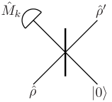
Fig. 1: The general scheme for converting one mixed state of zero and one photon to another.

The initial state is transformed by the beam splitter of transmissivity $t^{2}$ and reflectivity $r^{2}$ to $\hat{\rho}_{\rm BS}=E|{\phi}\rangle\langle{\phi}|+(1-E)|{00}\rangle$, with $|{\phi}\rangle=\alpha|{00}\rangle+\beta r|{10}\rangle+\beta t|{01}\rangle$. We begin by considering a projective measurement $|{Q}\rangle\langle{Q}|$. Projecting mode 1 onto a state $|{Q}\rangle$ will yield the unnormalized output state

$$\hat{\rho}^{\prime} =E[(\alpha\theta_{0}+\beta r\theta_{1})|{0}\rangle+\beta t\theta_{0}|{1}\rangle]\otimes{\rm H.c.}$$

$$\quad+(1-E)|\theta_{0}|^{2}|{0}\rangle\langle{0}|,$$ (2)

where $\theta_{j}=\langle{Q}|{j}\rangle$, from which we find

$$\beta^{\prime}(\alpha\theta_{0}+\beta r\theta_{1})=\alpha^{\prime}\beta t\theta_{0}.$$ (3)

The trace

$${\rm Tr}[\hat{\rho}^{\prime}]=E(|\alpha\theta_{0}+\beta r\theta_{1}|^{2}+|\beta t\theta_{0}|^{2})+(1-E)|\theta_{0}|^{2}$$ (4)

is equal to (proportional to in the case of $Q$ being a continuous observable) the probability for the desired measurement result to occur, and the efficiency of the output qubit is

$$E^{\prime}=E(|\alpha\theta_{0}+\beta r\theta_{1}|^{2}+|\beta t\theta_{0}|^{2})/{\rm Tr}[\hat{\rho}^{\prime}].$$ (5)

Using Eq. (3) as well as $\alpha^{2}+\beta^{2}=\alpha^{\prime 2}+\beta^{\prime 2}=1$, we simplify Eqs. (4) and (5) as follows:

$$t\beta\sqrt{E(1-E^{\prime})}=\beta^{\prime}\sqrt{E^{\prime}(1-E)},$$ (6)

$$p_{\rm success}\equiv{\rm Tr}[\hat{\rho}^{\prime}]=|\theta_{0}|^{2}(1-E)/(1-E^{\prime}).$$ (7)

Eq. (3) determines the efficiency-independent parameters of the output qubit that can be controlled by choosing the beam splitter and the measurement. An example is a field quadrature measurement using a homodyne detector[7]. With local oscillator phase $\phi$, result $Q$ gives the projection $\langle{Q_{\phi}}|$ satisfying (scaling convention is $[\hat{Q},\hat{P}]=i/2$)

$$\theta_{0}=\langle{Q_{\phi}}|{0}\rangle =\left(2/\pi\right)^{1/4}e^{-|Q|^{2}},$$

$$\theta_{1}=\langle{Q_{\phi}}|{1}\rangle =2Q\left(2/\pi\right)^{1/4}e^{-|Q|^{2}}e^{i\phi},$$ (8)

so $\theta_{1}/\theta_{0}=2Qe^{i\phi}$. With any beam splitter, by choosing appropriate $Q$ and $\phi$, one can obtain any desired qubit transformation except the transformation to vacuum. (The trivial transformation to vacuum may be obtained by taking $t=0$.)

We now turn to restrictions on the efficiency of the output qubit. We define the generalized efficiency by

$$\mathcal{E}(\hat{\rho})\equiv\frac{\rho_{11}}{1-|\rho_{01}|^{2}/\rho_{11}}=\frac{|\beta|^{2}E}{1-|\alpha|^{2}E},$$ (9)

where $\rho_{ij}=\langle{i}|\hat{\rho}|{j}\rangle$, and the $\rho_{ij}$ are given by

$$(\rho_{ij})=\left[\begin{array}[]{*{10}c}1-E|\beta|^{2}&E\alpha^{*}\beta\\ E\alpha\beta^{*}&E|\beta|^{2}\end{array}\right].$$ (10)

This efficiency has a number of useful properties: it is convex (see Appendix A); it reduces to $E$ for imperfect single photon sources ($\alpha=0$); $\mathcal{E}(\hat{\rho})=1$ corresponds to pure states, and $\mathcal{E}(\hat{\rho})=0$ corresponds to the vacuum state. Most importantly, since the beam splitter transmission cannot exceed one, Eq. (6) entails $\mathcal{E}(\hat{\rho})\geq\mathcal{E}(\hat{\rho}^{\prime})$. Hence only those transformations that do not increase the generalized efficiency are possible.

Furthermore (see Appendix B), our scheme with homodyne measurements permits any transformation that decreases the generalized efficiency. There is a complication for the case $\mathcal{E}(\hat{\rho})=1$ and $\mathcal{E}(\hat{\rho})>\mathcal{E}(\hat{\rho}^{\prime})$: a mixed state cannot be generated from a pure one using a projective measurement. In this case we can slightly attenuate the input state so its generalized efficiency reduces to a value between 1 and $\mathcal{E}(\hat{\rho}^{\prime})$. We can then transform the state to $\hat{\rho}^{\prime}$ using a second beam splitter and projective measurement. Mathematically, this procedure is equivalent to that of Fig. 1 with a POVM.

There are also two cases where it is possible to transform between states of equal generalized efficiency. These cases are:
Case 1: $\mathcal{E}(\hat{\rho})=\mathcal{E}(\hat{\rho}^{\prime})=1$
Case 2: $E=E^{\prime}$ and $|\beta|=|\beta^{\prime}|$
Case 1 corresponds to transforming between different pure states. Case 2 corresponds to a trivial phase shift, and also includes the trivial vacuum to vacuum transform. One can show (Appendix B) that these cases are the only ones where a transform between states of equal efficiency is possible.

We now generalize the obtained efficiency enhancement restriction to any scheme involving linear optics and conditional measurements (Fig. 2(a)). We assume that, first, there is only one nonclassical input: the single-rail qubit $\hat{\rho}$ and, second, the output state $\hat{\rho}^{\prime}$ has only zero- and one-photon terms in its Fock decomposition. Consider a processing scheme where the state is combined with any number of vacuum and coherent states at the input, then a POVM measurement is performed on all the modes except 1. A $U(N)$ interferometer can be decomposed into a line of beam splitters followed by a $U(N-1)$ interferometer[9]. The $U(N-1)$ interferometer can then be absorbed into the measurement, so the resulting interferometer is as in Fig. 2(b).

The beam splitters leave the coherent modes unentangled. One of these is an input to the last beam splitter, whereas a measurement is performed on the others. As these modes are not entangled, they may be omitted entirely, so there is only one coherent state input. In order to eliminate the multiphoton components in $\hat{\rho}^{\prime}$, the amplitude of this coherent state must be zero. The simplified configuration is then just as in Fig. 1.

We now recall that the measurement on mode 2 is generally not a projective measurement, but a POVM measurement. However, by a singular value decomposition, $\hat{M}_{k}=\sum p_{i}|{\sigma_{i}}\rangle\langle{Q_{i}}|$, where the $|{Q_{i}}\rangle$’s are orthogonal. The state $\hat{\rho}^{\prime}$ is thus a statistical mixture of outputs $\hat{\rho}^{\prime}_{i}$ associated with projections onto $|{Q_{i}}\rangle$. Because the generalized efficiency is convex (see Appendix A), we find $\forall i$ $\mathcal{E}(\hat{\rho}^{\prime})\leq\mathcal{E}(\hat{\rho}^{\prime}_{i})\leq\mathcal{E}(\hat{\rho})$, which completes the proof.

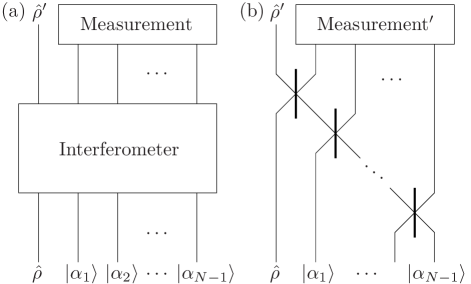
Fig. 2: (a) A general setup for transforming the state $\hat{\rho}$ to $\hat{\rho}^{\prime}$ involves an interferometer and a conditional measurement. (b) The same interferometer after absorbing all but a line of beam splitters into the measurement.

One application of our general scheme is to transform an incoherent mixture of the single-photon and vacuum states to a partially coherent state; this corresponds to the state preparation achieved by Refs. 3, 5, 7. A reverse transformation is also possible. In other words, the state $\hat{\rho}$ is equivalent to a photon source with efficiency $\mathcal{E}(\hat{\rho})$, in the sense that we may interconvert between these two states arbitrarily accurately. Therefore, it is reasonable to state that the generalized efficiency we have defined for mixed states with partial coherence is equivalent to the usual efficiency for single photon sources[8].

Whereas the generalized efficiency cannot be increased, it is possible to enhance the specific efficiency $E$ of a state, as demonstrated experimentally[7]. However, this will occur at the expense of the single-photon fraction $\beta$ in the qubit part of the state. It is not possible, for example, to enhance the efficiency of a single-photon source by first converting it into a single-rail qubit and then back into a single-photon state: while the efficiency may increase in the first step, it will reduce in the second step to no more than its original value.

Recently, Berry et al. proved for some special cases that it is impossible to enhance the efficiency of a single-photon source with any interferometric scheme such as in Fig. 2(a) but with an arbitrary number of inefficient single-photon inputs[10]. If this limitation is correct in general, the impossibility proof made in this paper would also be valid to the same degree of generality. Indeed, if there existed a scheme allowing one to conditionally convert an inefficient single-rail qubit $\hat{\rho}$ to another $\hat{\rho}^{\prime}$ so that $\mathcal{E}(\hat{\rho}^{\prime})>\mathcal{E}(\hat{\rho})$, one could use it to enhance the efficiency of a single-photon source. One would first set up a circuit as in Fig. 1 that converted the single photon to $\hat{\rho}$ with small loss of generalized efficiency, then transform $\hat{\rho}$ to $\hat{\rho}^{\prime}$ enhancing the generalized efficiency, then convert $\hat{\rho}^{\prime}$ back to a single-photon state.

In summary, we have presented a general state transformation scheme for single-rail qubits. This scheme uses only a beam splitter and conditional measurement, and includes existing experimental arrangements as special cases. We have also introduced a generalized measure of the efficiency of partially coherent mixed states of zero and one photon. This efficiency corresponds to the efficiency of imperfect single photon sources, because it is possible to reversibly convert between this state and a single photon source with arbitrarily low efficiency loss. Our scheme allows any transformation that decreases this generalized efficiency. Transformations that increase the efficiency are not possible, and transformations that keep the generalized efficiency constant are not possible, except for some trivial cases.

Appendix A: Convexity Proof. – Here we show that

$$\mathcal{E}(p\hat{\rho}_{1}+(1-p)\hat{\rho}_{2})\leq p\mathcal{E}(\hat{\rho}_{1})+(1-p)\mathcal{E}(\hat{\rho}_{2}),$$ (11)

for $p\in[0,1]$. If both $\hat{\rho}_{1}$ and $\hat{\rho}_{2}$ are the vacuum state, then clearly equality is achieved. If one of $\hat{\rho}_{1}$ and $\hat{\rho}_{2}$ is the vacuum state, then we can take that state to be $\hat{\rho}_{2}$ without loss of generality. Then, according to Eq. (10),

$$\mathcal{E}(p\hat{\rho}_{1}+(1-p)\hat{\rho}_{2}) =\frac{p|\beta|^{2}E}{1-p|\alpha|^{2}E}\leq\frac{p|\beta_{1}|^{2}E_{1}}{1-|\alpha_{1}|^{2}E_{1}}$$

$$=p\mathcal{E}(\hat{\rho}_{1})+(1-p)\mathcal{E}(\hat{\rho}_{2}).$$ (12)

For the case where neither state is the vacuum we define the function $f(p)=\mathcal{E}[p\hat{\rho}_{1}+(1-p)\hat{\rho}_{2}]$. Taking the second derivative of this function, we obtain

$$f^{\prime\prime}(p) =\frac{2\rho_{11}^{2}|\Delta\rho_{10}|^{2}}{(\rho_{11}-|\rho_{10}|^{2})^{2}}$$

$$\quad+\frac{2[\Delta\rho_{11}|\rho_{10}|^{2}-\rho_{11}2{\rm Re}(\rho_{01}\Delta\rho_{10})]^{2}}{(\rho_{11}-|\rho_{10}|^{2})^{3}},$$ (13)

where $\rho_{ij}=\langle{i}|[p\hat{\rho}_{1}+(1-p)\hat{\rho}_{2}]|{j}\rangle$ and $\Delta\rho_{ij}=\langle{i}|(\hat{\rho}_{1}-\hat{\rho}_{2})|{j}\rangle$. As neither state is the vacuum, this second derivative exists and is non-negative for $p\in[0,1]$. Hence $f(p)$ is convex, which implies Eq. (11). Thus, in each case we find that Eq. (11) holds, so the generalized efficiency is convex.

Appendix B: Optimality Proof. – We first show that transforms that decrease the generalized entropy are possible. If $\mathcal{E}(\hat{\rho})>\mathcal{E}(\hat{\rho}^{\prime})$, then $|\beta|^{2}E(1-E^{\prime})>|\beta^{\prime}|^{2}E^{\prime}(1-E)$, so there is a solution of Eq. (6) with $|t|<1$ and $r\neq 0$. If $\beta^{\prime}=0$, the transform can be obtained with $t=0$. If $\beta^{\prime}\neq 0$, then from Eq. (3) $\theta_{0}$ is also nonzero. The probability for success is then nonzero for $E<1$.

Now we show that the transformation that preserves the generalized efficiency is possible for Case 1 (Case 2 is trivial). For Case 1, $E=E^{\prime}=1$, so Eq. (6) is satisfied regardless of the value of $t$. Taking $t=r=1/\sqrt{2}$, $r\beta\beta^{\prime}\neq 0$, so $\theta_{0}\neq 0$. The probability of success is then $|\theta_{0}|^{2}(|t\alpha^{\prime}\beta/\beta^{\prime}|^{2}+|\beta t|^{2})$, which is nonzero, so the transformation is possible.

If $\mathcal{E}(\hat{\rho})=\mathcal{E}(\hat{\rho}^{\prime})$ but Cases 1 and 2 do not hold, then $|\beta|^{2}E(1-E^{\prime})=|\beta^{\prime}|^{2}E^{\prime}(1-E)$. For a projective measurement we obtain $|t|=1$, so $r=0$ and $t\alpha^{\prime}\beta\neq\alpha\beta^{\prime}$. Then Eq. (3) gives $\theta_{0}=0$, so the probability for success is zero.

References

- [1] A. P. Lund and T. C. Ralph, Phys. Rev. A 66, 032307 (2002).
- [2] T. C. Ralph, A. P. Lund, and H. M. Wiseman, quant-ph/0507192 (2005).
- [3] A. I. Lvovsky and J. Mlynek, Phys. Rev. Lett. 88, 250401 (2002).
- [4] D. T. Pegg, L. S. Phillips, and S. M. Barnett, Phys. Rev. Lett. 81, 1604 (1998).
- [5] S. A. Babichev, J. Ries, and A. I. Lvovsky, Europhys. Lett. 64, 1 (2003).
- [6] C. H. Bennett, G. Brassard, C. Crépeau, R. Jozsa, A. Peres, and W. K. Wootters, Phys. Rev. Lett. 70, 1895 (1993).
- [7] S. A. Babichev, B. Brezger, and A. I. Lvovsky, Phys. Rev. Lett. 92, 047903 (2004).
- [8] A. I. Lvovsky, H. Hansen, T. Aichele, O. Benson, J. Mlynek, and S. Schiller, Phys. Rev. Lett. 87, 050402 (2001).
- [9] D. W. Berry, S. Scheel, C. R. Myers, B. C. Sanders, P. L. Knight, and R. Laflamme, New J. Phys. 6, 93 (2004).
- [10] D. W. Berry, S. Scheel, B. C. Sanders, and P. L. Knight, Phys. Rev. A 69, 031806 (2004).