Topology of the three-qubit space of entanglement types

Abstract

The three-qubit space of entanglement types is the orbit space of the local unitary action on the space of three-qubit pure states, and hence describes the types of entanglement that a system of three qubits can achieve. We show that this orbit space is homeomorphic to a certain subspace of $\mathbb{R}^{6}$, which we describe completely. We give a topologically based classification of three-qubit entanglement types, and we argue that the nontrivial topology of the three-qubit space of entanglement types forbids the existence of standard states with the convenient properties of two-qubit standard states.

I Introduction

Quantum entanglement is an important resource in quantum computation, quantum communication, and other emerging quantum technologies. A fundamental problem in quantum entanglement theory is to understand the types of entanglement that a composite quantum system can achieve.

Linden and Popescu Linden and Popescu (1998) presented a program for precisely characterizing the types of entanglement that a composite quantum system can exhibit. In their program, the Lie group of local unitary (LU) transformations acts on the space of quantum states, partitioning it into orbits. Each orbit represents a type of entanglement achievable by the quantum system. The collection of orbits, known as the orbit space (see, for example, Hatcher (2002), p. 72) or the space of entanglement types, then forms a mathematical object that describes all of the possible types of entanglement for a quantum system. In fact, Linden and Popescu regarded this orbit space as “the main mathematical object we are investigating.”Linden and Popescu (1998) They went on to determine the number of parameters required to distinguish orbits in the orbit space and to comment on the importance of local unitary invariants in describing the orbit space.

In Linden et al. (1999), Linden, Popescu, and Sudbery gave the number of parameters needed to describe the space of entanglement types for mixed quantum states, and emphasized the importance of having enough LU invariants to separate orbits. (A collection of invariants separates orbits if any two states with the same values for each invariant necessarily lie on the same orbit. Such a collection is also called a complete set of invariants.)

Kempe Kempe (1999), Coffman et al. Coffman et al. (2000), and Sudbery Sudbery (2001) identified specific LU invariants for three-qubit pure states.

A major advance toward a complete description of the three-qubit space of entanglement types came from Acín et al. Acín et al. (2000, 2001) who found a standard form for three-qubit state vectors and a convenient set of LU invariants that had a simple form when evaluated for standard state vectors. The near invertibility of their expressions for invariants allowed Acín et al. to argue that a set of six LU invariants were sufficient to separate orbits, giving unique coordinates for the orbit space. The allowable values that the invariants could assume remained unknown, and consequently the understanding of the types of entanglement achievable for three qubits was incomplete.

An additional point that deserves to be emphasized is that the space $\mathcal{E}$ of entanglement types is a topological space, and not merely a set. Topology provides a system for keeping track of which types of entanglement are “close” to other types. Thus we define the space of entanglement types for $n$ qubits, $\mathcal{E}_{n}$, to be the orbit space produced by the action of the local unitary group on the $n$-qubit pure quantum state space. In other words, $\mathcal{E}_{n}$ is the set of LU orbits (entanglement types) equipped with the quotient topology it inherits from the quantum state space.

The present work completes Linden and Popescu’s program for three-qubit pure states. We precisely characterize $\mathcal{E}_{3}$, showing that it is homeomorphic (identical not just as a set but as a topological space) to a particular subspace of $\mathbb{R}^{6}$.

The paper is organized as follows. In section II, we give a general program for describing the space of entanglement types for a composite quantum system as a topological space. In section III, we apply this program to two-qubit pure states in an effort to gain some insight in a simple setting. Section IV applies the general program to three-qubit pure states, and constitutes the heart of the paper. Section V provides some help in visualizing the possibilities for three-qubit entanglement types, and gives a topologically based classification. In section VI, we argue that the nontrivial topology of $\mathcal{E}_{3}$ forbids the existence of three-qubit standard states possessing all of the nice properties that two-qubit standard states have.

II Space of Entanglement Types

In this section, we outline a general program for describing the space of entanglement types of a composite quantum system as a topological imbedding (see, for example, Munkres (2000), p. 105) in $\mathbb{R}^{m}$ for some $m$.

Let $H=\mathbb{C}^{d}$ denote the Hilbert space of a quantum system. Quantum states correspond to rays in the Hilbert space, so the space of quantum states is $\mathbb{P}(\mathbb{C}^{d})=\mathbb{CP}^{d-1}$, the $(d-1)$-dimensional complex projective space. The $(2d-1)$-sphere, $S^{2d-1}$, is the collection of normalized state vectors in $\mathbb{R}^{2d}\approx\mathbb{C}^{d}$. Let $T$ be the space on which the group of LU transformations acts. If the group $G$ of LU transformations contains operations that change the phase of state vectors (as the groups $U(2)\times U(2)\times U(2)$ and $SU(2)\times SU(2)\times SU(2)\times U(1)$ do for three qubits), then it does not matter whether the orbit space is formed from the space of quantum states or from the space of normalized quantum state vectors. In the notation of Hatcher (2002), the definition of the space of entanglement types is

$$\mathcal{E}\equiv T/G=\mathbb{CP}^{d-1}/G=S^{2d-1}/G.$$

In the sequel, we require the space $T$ to be topologically compact. Both $\mathbb{CP}^{d-1}$ and $S^{2d-1}$ are compact, and both lead to the correct orbit space, so either may be chosen for the space $T$. For mixed states, one could take $T$ to be the space of density matrices.

Proposition 1

Let $(I_{1},\dots,I_{m})$ be a complete set of continuous, real-valued invariants. Applying the collection of invariants to a quantum state provides a continuous map $I:T\to\mathbb{R}^{m}$. If $X\subset\mathbb{R}^{m}$ is the image of this map, then the space $\mathcal{E}$ of entanglement types is homeomorphic to $X$.

Proof. Since the map $I$ is constructed from LU invariants, it must factor through the space $\mathcal{E}$ of entanglement types: $I=f\circ\pi$, where $\pi$ is the projection map that associates a quantum state with its entanglement type in $\mathcal{E}$. (The map $f$ is well defined because $I$ is constructed from LU invariants.)

Since there are enough LU invariants to separate orbits, the map $f$ is one-to-one, and since $X$ is the image of the map $I$, the map $f$ is onto. The map $\pi$ is continuous since it defines the quotient topology on $\mathcal{E}$, and $I$ is continuous because its components are continuous, so $f$ is continuous by a standard result about quotient spaces (see Munkres (2000), Theorem 22.2). The map $f:\mathcal{E}\to X$ is then a continuous bijection. Since $\mathcal{E}$ is compact (it is the image of the compact space $T$ under the continuous map $\pi$) and $X$ is Hausdorff (a subspace of a Hausdorff space is Hausdorff), we have that $f$ is a homeomorphism. (See, for example, Munkres (2000), Theorem 26.6.) $\square$

III Description of $\mathcal{E}_{2}$

In this section, we apply the procedure of the previous section to pure states of two qubits to see how it works in a familiar setting. For pure states of two qubits, the Hilbert space is $\mathbb{C}^{2}\otimes\mathbb{C}^{2}\approx\mathbb{C}^{4}$, the quantum state space is $\mathbb{P}(\mathbb{C}^{2}\otimes\mathbb{C}^{2})\approx\mathbb{CP}^{3}$, and the space of normalized quantum state vectors is $S^{7}$. The group of local unitary transformations is $U(2)\times U(2)$. The space of entanglement types is

$$\mathcal{E}_{2}=\mathbb{P}(\mathbb{C}^{2}\otimes\mathbb{C}^{2})/U(2)\times U(2)=S^{7}/U(2)\times U(2).$$

A single LU invariant is all that is required to separate orbits for pure states of two qubits. For a normalized two-qubit pure state

$$\left|\psi\right\rangle=\sum_{i=0}^{1}\sum_{j=0}^{1}\psi_{ij}\left|ij\right\rangle,$$

the concurrence introduced by Hill and Wootters Hill and Wootters (1997),

$$C(\psi)=2\left|\psi_{00}\psi_{11}-\psi_{01}\psi_{10}\right|,$$

is a continuous, real-valued invariant. The Schmidt decomposition theorem Ekert and Knight (1995); Aravind (1996) tells us that this single invariant is sufficient to separate orbits, so it suffices to use $m=1$ invariant for two qubits. It is easily shown that the image of the concurrence map is $[0,1]\subset\mathbb{R}^{1}$, the closed interval from zero to one. We conclude that $\mathcal{E}_{2}$ is homeomorphic to $[0,1]$. Two-qubit entanglement types are in one-to-one correspondence with the closed unit interval, with $0$ representing unentangled states, $1$ representing fully entangled states, and numbers in the open unit interval representing varying degrees of partially entangled states.

Table 1 gives a topologically based classification of two-qubit entanglement types, provided mainly for later comparison with Table 2 which classifies three-qubit entanglement types. In this table, we view $\mathcal{E}_{2}$ as a cell complex (or CW complex) Hatcher (2002) composed of two 0-cells (points) and one 1-cell (open unit interval). One 0-cell, $e^{0}_{SEP}$, represents the separable (unentangled) states. The other 0-cell, $e^{0}_{EPR}$, represents fully entangled states, such as the EPR pair, $\left|EPR\right\rangle=1/\sqrt{2}(\left|01\right\rangle-\left|10\right\rangle)$. The 1-cell, $e^{1}$, representing all of the partial entanglement types is attached to $e^{0}_{SEP}$ at one end and to $e^{0}_{EPR}$ at the other end.

Entanglement types considered in the present work are more precisely called LU entanglement types, since each type is associated with an equivalence class of quantum states under local unitary transformation. An alternative equivalence relation on the space of quantum states is is equivalence under stochastic local operations and classical communication (SLOCC) Dür et al. (2000). Each SLOCC equivalence class of quantum states can be regarded as an SLOCC entanglement type in the same way that each LU equivalence class of quantum states is regarded as an LU entanglement type. For two-qubit pure states, there are only two SLOCC classes: unentangled and entangled. LU operations are a subset of SLOCC operations, so each LU entanglement type that we have identified is associated with exactly one SLOCC entanglement type. In Table 1, we list the SLOCC class associated with each collection of LU entanglement types.

Each LU entanglement type corresponds to an LU orbit (an equivalence class) of quantum states. This LU orbit is a differentiable manifold of quantum states. The fourth column of Table 1 lists the dimension of the LU orbit of quantum states for each entanglement type Kuś and Życzkowski (2001); Walck .

Table 1: Two-qubit space of entanglement types viewed as a cell complex. The superscript in the cell name gives the dimension of the cell.

Cell		SLOCC	Orbit
name	Concurrence	Class	Dimension
$e^{0}_{SEP}$	$C(\psi)=0$	unentangled	4
$e^{1}$	$0<C(\psi)<1$	entangled	5
$e^{0}_{EPR}$	$C(\psi)=1$	entangled	3

IV Description of $\mathcal{E}_{3}$

In this section, we apply the procedure of section II to pure states of three qubits. For pure states of three qubits, the Hilbert space is $\mathbb{C}^{2}\otimes\mathbb{C}^{2}\otimes\mathbb{C}^{2}\approx\mathbb{C}^{8}$, the quantum state space is $\mathbb{P}(\mathbb{C}^{2}\otimes\mathbb{C}^{2}\otimes\mathbb{C}^{2})\approx\mathbb{CP}^{7}$, and the space of normalized quantum state vectors is $S^{15}$. The group of local unitary transformations is $U(2)\times U(2)\times U(2)$. The space of entanglement types is

$$\mathcal{E}_{3} =\mathbb{P}(\mathbb{C}^{2}\otimes\mathbb{C}^{2}\otimes\mathbb{C}^{2})/U(2)\times U(2)\times U(2)$$

$$=S^{15}/U(2)\times U(2)\times U(2).$$

Let

$$\left|\psi\right\rangle=\sum_{i=0}^{1}\sum_{j=0}^{1}\sum_{k=0}^{1}\psi_{ijk}\left|ijk\right\rangle$$

denote a normalized three-qubit state vector. We will use the symbol $\psi$ without ket notation to denote the column vector of coefficients $\psi_{ijk}$ in the standard basis.

In order to apply the program of section II, our first step is to choose some LU invariants. Let $n$ be a positive integer, and let $\sigma$ and $\tau$ be permutations on $n$ elements. For each $n$, $\sigma$, and $\tau$, define a function $P_{\sigma,\tau}^{n}:\mathbb{C}^{8}\to\mathbb{C}$ by

$$P_{\sigma,\tau}^{n}(\psi)=\sum_{i_{1}=0}^{1}\sum_{j_{1}=0}^{1}\sum_{k_{1}=0}^{1}\cdots\sum_{i_{n}=0}^{1}\sum_{j_{n}=0}^{1}\sum_{k_{n}=0}^{1}\psi_{i_{1}j_{1}k_{1}}\cdots\psi_{i_{n}j_{n}k_{n}}\psi_{i_{1}j_{\sigma(1)}k_{\tau(1)}}^{*}\cdots\psi_{i_{n}j_{\sigma(n)}k_{\tau(n)}}^{*}$$ (1)

Every function of this form is an LU invariant Sudbery (2001); Weyl (1939); Gingrich (2002). Define

$$I_{1}(\psi) =P_{e,(12)}^{2}(\psi)$$

$$I_{2}(\psi) =P_{(12),e}^{2}(\psi)$$

$$I_{3}(\psi) =P_{(12),(12)}^{2}(\psi)$$

$$I_{4}(\psi) =P_{(123),(132)}^{3}(\psi)$$

$$I_{5}(\psi) =\left|\operatorname{Hdet}(\psi)\right|^{2}$$

$$I_{6}(\psi) =\operatorname{Im}[P_{(34)(56),(13524)}^{6}(\psi)]$$

Invariants $I_{1}$ through $I_{4}$ match those given in Gingrich (2002). It is straightforward to show that they are real-valued invariants. $\operatorname{Hdet}$ is Cayley’s hyperdeterminant used in Acín et al. (2000) and corresponding to the three-tangle of Coffman et al. (2000); Sudbery (2001).

The authors of Acín et al. (2000, 2001); Gingrich (2002) chose a discrete invariant as a sixth invariant in an effort to avoid redundancy. Because we are interested in topology and we want to preserve the information about which orbits are close to other orbits, we choose $I_{6}$ to be a continuous invariant rather than a discrete one.

Acín and coworkers Acín et al. (2000, 2001) introduced a new set of invariants that made it possible to argue that the invariants separate orbits.

$$J_{1}(\psi) =\frac{1}{4}\left[1-I_{1}(\psi)-I_{2}(\psi)+I_{3}(\psi)-2\sqrt{I_{5}(\psi)}\right]$$ (2)

$$J_{2}(\psi) =\frac{1}{4}\left[1-I_{1}(\psi)+I_{2}(\psi)-I_{3}(\psi)-2\sqrt{I_{5}(\psi)}\right]$$ (3)

$$J_{3}(\psi) =\frac{1}{4}\left[1+I_{1}(\psi)-I_{2}(\psi)-I_{3}(\psi)-2\sqrt{I_{5}(\psi)}\right]$$ (4)

$$J_{4}(\psi) =\sqrt{I_{5}(\psi)}$$ (5)

$$J_{5}(\psi) =\frac{5}{12}-\frac{1}{4}I_{1}(\psi)-\frac{1}{4}I_{2}(\psi)-\frac{1}{4}I_{3}(\psi)$$

$$\hskip 14.22636pt+\frac{1}{3}I_{4}(\psi)-\frac{1}{2}\sqrt{I_{5}(\psi)}$$ (6)

$$J_{6}(\psi) =I_{6}(\psi)$$ (7)

Invariants $J_{1}$ through $J_{5}$ match those given in both Acín et al. (2000, 2001) and Gingrich (2002).

The invariants $J_{i}$ have nice properties under qubit permutation. Invariant $J_{1}$, which reports on the two-qubit entanglement between qubits 2 and 3, is invariant under interchange of qubits 2 and 3. Similarly, $J_{2}$ ($J_{3}$) is invariant under interchange of qubits 1 and 3 (1 and 2). LU invariants $J_{4}$, $J_{5}$, and $J_{6}$ encode the essential three-qubit entanglement of the state, and remain unchanged under any permutation of qubits.

Acín et al. Acín et al. (2000, 2001) generalized the Schmidt decomposition to three qubits, showing that every normalized three-qubit state vector is LU-equivalent to a standard state vector of the form

$$\left|\chi\right\rangle=\lambda_{0}\left|000\right\rangle+\lambda_{1}e^{i\phi}\left|100\right\rangle+\lambda_{2}\left|101\right\rangle+\lambda_{3}\left|110\right\rangle+\lambda_{4}\left|111\right\rangle,$$ (8)

where the $\lambda_{i}$ are real and nonnegative, $\phi$ is real, and $\sum_{i=0}^{4}\lambda_{i}^{2}=1$. Evaluating invariants (2)–(7) for the standard state vector $\chi$, we have Acín et al. (2000, 2001); Gingrich (2002)

$$J_{1}(\chi) =\left|\lambda_{1}\lambda_{4}e^{i\phi}-\lambda_{2}\lambda_{3}\right|^{2}$$ (9)

$$J_{2}(\chi) =\lambda_{0}^{2}\lambda_{2}^{2}$$ (10)

$$J_{3}(\chi) =\lambda_{0}^{2}\lambda_{3}^{2}$$ (11)

$$J_{4}(\chi) =\lambda_{0}^{2}\lambda_{4}^{2}$$ (12)

$$J_{5}(\chi) =2\lambda_{0}^{2}\lambda_{2}^{2}\lambda_{3}^{2}-2\lambda_{0}^{2}\lambda_{1}\lambda_{2}\lambda_{3}\lambda_{4}\cos\phi$$ (13)

$$J_{6}(\chi) =\lambda_{0}^{4}\lambda_{1}\lambda_{2}\lambda_{3}\lambda_{4}\sin\phi$$

$$\hskip 14.22636pt\times(2\lambda_{0}^{2}\lambda_{4}^{2}+2\lambda_{1}^{2}\lambda_{4}^{2}-\lambda_{4}^{2}-2\lambda_{1}\lambda_{2}\lambda_{3}\lambda_{4}\cos\phi).$$ (14)

Invariants $J_{1}$ through $J_{6}$ are a complete set of continuous, real-valued invariants. If we can find the image in $\mathbb{R}^{6}$ that these invariants make, then by Proposition 1, we can completely characterize the space of entanglement types for three qubits. The next proposition does this.

Proposition 2

The three-qubit space of entanglement types, $\mathcal{E}_{3}$, is homeomorphic to the subspace of $\mathbb{R}^{6}$ consisting of points $(\beta_{1},\beta_{2},\beta_{3},\beta_{4},\beta_{5},\beta_{6})\in\mathbb{R}^{6}$ that satisfy

$$0 \leq\beta_{1}\leq\frac{1}{4},$$ (15)

$$0 \leq\beta_{2}\leq\frac{1}{4},$$ (16)

$$0 \leq\beta_{3}\leq\frac{1}{4},$$ (17)

$$0 \leq\beta_{4}\leq\frac{1}{4},$$ (18)

$$\beta_{1}\beta_{2}+\beta_{1}\beta_{3}+\beta_{2}\beta_{3}+(\beta_{1}+\beta_{2}+\beta_{3})\beta_{4}+\beta_{4}^{2}\leq\frac{1}{4}\beta_{4}+\frac{1}{2}\beta_{5},$$ (19)

and

$$\left[(\beta_{5}+\beta_{4})^{2}-4(\beta_{1}+\beta_{4})(\beta_{2}+\beta_{4})(\beta_{3}+\beta_{4})\right]\\ \times\left[\beta_{5}^{2}-4\beta_{1}\beta_{2}\beta_{3}\right]+4\beta_{6}^{2}=0.$$ (20)

Proof. Define a map $J:S^{15}\to\mathbb{R}^{6}$ by

$$J(\psi)=\left(J_{1}(\psi),J_{2}(\psi),J_{3}(\psi),J_{4}(\psi),J_{5}(\psi),J_{6}(\psi)\right).$$

Let $X$ be the subspace of $\mathbb{R}^{6}$ satisfying conditions (15)–(20) above.

We claim that $X$ is the image of the map $J$. From this and Proposition 1 we may conclude that $X$ is homeomorphic to $\mathcal{E}_{3}$. We will show first that $J$ maps into $X$ (so that $X$ contains the image of $J$), and then that $J$ maps onto $X$ (so that $X$ is contained in the image of $J$).

Before we proceed with main part of the proof, we wish to note some conditions that are implied by conditions (15)–(20) above.

$$\beta_{4}+\beta_{5}\geq 0$$ (21)

$$\beta_{5}^{2}-4\beta_{1}\beta_{2}\beta_{3}\leq 0$$ (22)

$$\Delta_{\beta}\equiv(\beta_{5}+\beta_{4})^{2}-4(\beta_{1}+\beta_{4})(\beta_{2}+\beta_{4})(\beta_{3}+\beta_{4})\geq 0$$ (23)

Condition (21) follows from (19) and the fact that $\beta_{1}$, $\beta_{2}$, $\beta_{3}$, and $\beta_{4}$ are nonnegative. To establish (22), assume the contrary, that $\beta_{5}^{2}-4\beta_{1}\beta_{2}\beta_{3}>0$. Equation (20) then requires that $4(\beta_{1}+\beta_{4})(\beta_{2}+\beta_{4})(\beta_{3}+\beta_{4})-(\beta_{5}+\beta_{4})^{2}\geq 0$, and adding these two inequalities violates (19). Hence (22) is established. To establish (23), assume the contrary, that $4(\beta_{1}+\beta_{4})(\beta_{2}+\beta_{4})(\beta_{3}+\beta_{4})-(\beta_{5}+\beta_{4})^{2}>0$. Equation (20) then requires that $\beta_{5}^{2}-4\beta_{1}\beta_{2}\beta_{3}\geq 0$, and adding these two inequalities violates (19). Hence (23) is established.

To show that $J$ maps into $X$, we must show that $J(\psi)\in X$ for all normalized three-qubit state vectors $\psi$. In other words, if $\beta=J(\psi)$ for a normalized three-qubit state vector $\psi$, then $\beta=(\beta_{1},\beta_{2},\beta_{3},\beta_{4},\beta_{5},\beta_{6})$ satisfies conditions (15)–(20) above.

In Acín et al. (2001), Acín et al. record conditions (15)–(18) as well as (23), so we will assume these and move on to prove (19) and (20). Let $\beta=J(\psi)$ for a normalized three-qubit state vector $\psi$. Let $\chi$ be a three-qubit state vector in standard form (8) that is LU-equivalent to $\psi$. Then $\beta=J(\chi)$.

Let us prove (19) for $\beta=J(\psi)$. Our approach is to prove (22), and then to use (22) and (23) to prove (19). For condition (22), equations (9), (10), (11), and (13) give

$$\beta_{1}\beta_{2}\beta_{3}-\frac{\beta_{5}^{2}}{4}=\lambda_{0}^{4}\lambda_{1}^{2}\lambda_{2}^{2}\lambda_{3}^{2}\lambda_{4}^{2}\sin^{2}\phi\geq 0.$$ (24)

If $\beta_{4}>0$, then (19) is obtained by subtracting (22) from (23), and dividing by $\beta_{4}$. If $\beta_{4}=0$, we must show that

$$\beta_{1}\beta_{2}+\beta_{1}\beta_{3}+\beta_{2}\beta_{3}\leq\frac{1}{2}\beta_{5}.$$ (25)

By equation (12), either $\lambda_{0}=0$ or $\lambda_{4}=0$. If $\lambda_{0}=0$, then equations (10), (11), and (13) show that $\beta_{2}=\beta_{3}=\beta_{5}=0$, and (25) is satisfied. Alternatively, if $\lambda_{4}=0$, then equations (9), (10), (11), and (13) give

$$\beta_{1}\beta_{2}+\beta_{1}\beta_{3}+\beta_{2}\beta_{3}=\lambda_{0}^{2}\lambda_{2}^{2}\lambda_{3}^{2}(\lambda_{0}^{2}+\lambda_{2}^{2}+\lambda_{3}^{2})\leq\frac{1}{2}\beta_{5}.$$

This completes the proof of condition (19) for $\beta=J(\psi)$.

For condition (20), note from equations (9)–(13) that

$$(\beta_{4}+\beta_{5})^{2}-4(\beta_{1}+\beta_{4})(\beta_{2}+\beta_{4})(\beta_{3}+\beta_{4})\\ =\lambda_{0}^{4}(2\lambda_{0}^{2}\lambda_{4}^{2}+2\lambda_{1}^{2}\lambda_{4}^{2}-\lambda_{4}^{2}-2\lambda_{1}\lambda_{2}\lambda_{3}\lambda_{4}\cos\phi)^{2}.$$ (26)

This, along with equations (24) and (14) gives condition (20). This completes the proof for the claim that $J$ maps into $X$.

Next we address the claim that $J$ maps onto $X$. Here we must show for any $\beta\in X$ that there exists a normalized three-qubit state vector $\psi$ such that $J(\psi)=\beta$. In fact we will produce a normalized three-qubit state vector $\chi$ in standard form (8) such that $J(\chi)=\beta$.

• Case 1: $\beta_{1}+\beta_{4}=0$. In this case, conditions (15) and (18) imply that $\beta_{1}=0$ and $\beta_{4}=0$. Condition (22) then implies that $\beta_{5}=0$, condition (20) implies that $\beta_{6}=0$, and conditions (16), (17), and (19) imply that $\beta_{2}\beta_{3}=0$.

• Case 1a: $\beta_{2}=0$. Let

  $$\left|\chi\right\rangle=\sqrt{\frac{1}{2}+\sqrt{\frac{1}{4}-\beta_{3}}}\left|000\right\rangle+\sqrt{\frac{1}{2}-\sqrt{\frac{1}{4}-\beta_{3}}}\left|110\right\rangle.$$ (27)

  Notice that condition (17) guarantees real nonnegative entries for $\chi$.

• Case 1b: $\beta_{3}=0$. Let

  $$\left|\chi\right\rangle=\sqrt{\frac{1}{2}+\sqrt{\frac{1}{4}-\beta_{2}}}\left|000\right\rangle+\sqrt{\frac{1}{2}-\sqrt{\frac{1}{4}-\beta_{2}}}\left|101\right\rangle.$$ (28)

  Notice that condition (16) guarantees real nonnegative entries for $\chi$.

• Case 2: $\beta_{1}+\beta_{4}>0$. Let

  $$\lambda_{0}^{2}=\frac{\beta_{4}+\beta_{5}+\sqrt{\Delta_{\beta}}}{2(\beta_{1}+\beta_{4})}.$$ (29)

  Conditions (21) and (23) imply that $\lambda_{0}^{2}$ is nonnegative. Choose $\lambda_{0}$ to be nonnegative.

• Case 2a: $\lambda_{0}=0$. Condition (21) implies that $\beta_{4}+\beta_{5}=0$. Condition (23), along with conditions (15), (16), (17), and (18), then implies that $\beta_{4}=0$ (and hence that $\beta_{5}=0$), and also that $\beta_{1}\beta_{2}\beta_{3}=0$. Condition (20) implies that $\beta_{6}=0$. We must have $\beta_{1}>0$, and then condition (19) implies $\beta_{2}=\beta_{3}=0$. Let

  $$\left|\chi\right\rangle=\sqrt{\frac{1}{2}+\sqrt{\frac{1}{4}-\beta_{1}}}\left|100\right\rangle+\sqrt{\frac{1}{2}-\sqrt{\frac{1}{4}-\beta_{1}}}\left|111\right\rangle.$$ (30)

  Notice that condition (15) guarantees real nonnegative entries for $\chi$.

• Case 2b: $\lambda_{0}>0$. Let

  $$\lambda_{2}=\frac{\sqrt{\beta_{2}}}{\lambda_{0}},\hskip 14.22636pt\lambda_{3}=\frac{\sqrt{\beta_{3}}}{\lambda_{0}},\hskip 14.22636pt\lambda_{4}=\frac{\sqrt{\beta_{4}}}{\lambda_{0}}.$$

• Case 2b1: $\beta_{4}=0$. Since Case 2 requires $\beta_{1}+\beta_{4}>0$, we have $\beta_{1}>0$. Conditions (22) and (23) imply that $\Delta_{\beta}=0$, and hence that

  $$\lambda_{0}^{2}=\frac{\beta_{5}}{2\beta_{1}}.$$

  Since Case 2b requires $\lambda_{0}>0$, we must have $\beta_{5}>0$. Let

  $$\left|\chi\right\rangle=\sqrt{\frac{\beta_{5}}{2\beta_{1}}}\left|000\right\rangle+\sqrt{1-\frac{\beta_{5}}{2\beta_{1}}-\frac{2\beta_{1}\beta_{2}}{\beta_{5}}-\frac{2\beta_{1}\beta_{3}}{\beta_{5}}}\left|100\right\rangle\\ +\sqrt{\frac{2\beta_{1}\beta_{2}}{\beta_{5}}}\left|101\right\rangle+\sqrt{\frac{2\beta_{1}\beta_{3}}{\beta_{5}}}\left|110\right\rangle.$$ (31)

  Also note that when $\beta_{4}=0$, conditions (22) and (23) imply that

  $$\beta_{5}=2\sqrt{\beta_{1}\beta_{2}\beta_{3}}.$$ (32)

  Condition (20) then implies that $\beta_{6}=0$. When $\beta_{4}=0$, condition (19) becomes (25). Multiplying the latter by $2/\beta_{5}$ and using (32), we get

  $$\frac{2\beta_{1}\beta_{2}}{\beta_{5}}+\frac{2\beta_{1}\beta_{3}}{\beta_{5}}+\frac{\beta_{5}}{2\beta_{1}}\leq 1,$$

  which shows that all of the entries in $\chi$ above are real and nonnegative.

• Case 2b2: $\beta_{4}>0$, $\beta_{2}=0$. Condition (22) implies that $\beta_{5}=0$. Condition (20) implies that $\beta_{6}=0$. Let

  $$\left|\chi\right\rangle=\lambda_{0}\left|000\right\rangle+\lambda_{0}\sqrt{\frac{\beta_{1}}{\beta_{4}}}\left|100\right\rangle+\frac{\sqrt{\beta_{3}}}{\lambda_{0}}\left|110\right\rangle+\frac{\sqrt{\beta_{4}}}{\lambda_{0}}\left|111\right\rangle,$$

  where $\lambda_{0}$ is given by (29). The entries in $\chi$ are clearly nonnegative.

• Case 2b3: $\beta_{4}>0$, $\beta_{3}=0$. Condition (22) implies that $\beta_{5}=0$. Condition (20) implies that $\beta_{6}=0$. Let

  $$\left|\chi\right\rangle=\lambda_{0}\left|000\right\rangle+\lambda_{0}\sqrt{\frac{\beta_{1}}{\beta_{4}}}\left|100\right\rangle+\frac{\sqrt{\beta_{2}}}{\lambda_{0}}\left|101\right\rangle+\frac{\sqrt{\beta_{4}}}{\lambda_{0}}\left|111\right\rangle,$$

  where $\lambda_{0}$ is given by (29). The entries in $\chi$ are clearly nonnegative.

• Case 2b4: $\beta_{2}\beta_{3}\beta_{4}>0$, $\Delta_{\beta}=0$. Condition (20) implies that $\beta_{6}=0$. Let

  $$\left|\chi\right\rangle=\lambda_{0}\left|000\right\rangle\\ +\left(\frac{2\beta_{2}\beta_{3}-\lambda_{0}^{2}\beta_{5}}{2\lambda_{0}\sqrt{\beta_{2}\beta_{3}\beta_{4}}}+i\lambda_{0}\frac{\sqrt{\beta_{1}\beta_{2}\beta_{3}-\beta_{5}^{2}/4}}{\sqrt{\beta_{2}\beta_{3}\beta_{4}}}\right)\left|100\right\rangle\\ +\frac{\sqrt{\beta_{2}}}{\lambda_{0}}\left|101\right\rangle+\frac{\sqrt{\beta_{3}}}{\lambda_{0}}\left|110\right\rangle+\frac{\sqrt{\beta_{4}}}{\lambda_{0}}\left|111\right\rangle,$$ (33)

  where $\lambda_{0}$ is given by (29). The entries are all well defined since $\lambda_{0}>0$ in Case 2b. Note also that $\lambda_{0}$, $\lambda_{2}$, $\lambda_{3}$, and $\lambda_{4}$ are nonnegative.

• Case 2b5: $\beta_{2}\beta_{3}\beta_{4}>0$, $\Delta_{\beta}>0$. Let

  $$\left|\chi\right\rangle=\lambda_{0}\left|000\right\rangle\\ +\left(\frac{2\beta_{2}\beta_{3}-\lambda_{0}^{2}\beta_{5}}{2\lambda_{0}\sqrt{\beta_{2}\beta_{3}\beta_{4}}}+i\lambda_{0}\frac{\beta_{6}}{\sqrt{\beta_{2}\beta_{3}\beta_{4}\Delta_{\beta}}}\right)\left|100\right\rangle\\ +\frac{\sqrt{\beta_{2}}}{\lambda_{0}}\left|101\right\rangle+\frac{\sqrt{\beta_{3}}}{\lambda_{0}}\left|110\right\rangle+\frac{\sqrt{\beta_{4}}}{\lambda_{0}}\left|111\right\rangle,$$ (34)

  where $\lambda_{0}$ is given by (29). The entries are all well defined since $\lambda_{0}>0$ in Case 2b. Note also that $\lambda_{0}$, $\lambda_{2}$, $\lambda_{3}$, and $\lambda_{4}$ are nonnegative.

In each case, a bit of algebra shows that $\chi$ is normalized. Using (9)–(14), one can show that $J(\chi)=\beta$. $\square$

V Visualization of $\mathcal{E}_{3}$

The description of $\mathcal{E}_{3}$ given by Proposition 2 is precise and complete; nevertheless we want a way to visualize the possibilities for three-qubit entanglement. One way to proceed is to create a hierarchy of the six invariants we used in describing orbits. At the top of our hierarchy we choose $\beta_{4}$. Our $\beta_{4}$ is related to the 3-tangle of Coffman et al. (2000), and controls the amount of “GHZ entanglement” possessed by a state. If any qubit is unentangled from the other two, then $\beta_{4}=0$, and if $\beta_{4}=1/4$, its maximum value, the three qubits have the type of entanglement possessed by the GHZ state, $\left|GHZ\right\rangle=1/\sqrt{2}(\left|000\right\rangle+\left|111\right\rangle)$.

We first consider the entanglement possibilities for $\beta_{4}=0$. When $\beta_{4}=0$, conditions (21), (22), and (23) imply that $\beta_{5}=2\sqrt{\beta_{1}\beta_{2}\beta_{3}}$ and condition (20) then implies that $\beta_{6}=0$. Condition (19) becomes

$$\beta_{1}\beta_{2}+\beta_{1}\beta_{3}+\beta_{2}\beta_{3}\leq\sqrt{\beta_{1}\beta_{2}\beta_{3}}.$$ (35)

The allowable values for $\beta_{1}$, $\beta_{2}$, and $\beta_{3}$ are given by (15), (16), (17), and (35). The entanglement types when $\beta_{4}=0$ are shown in Figure 1. They fill a region in $\beta_{1}$,$\beta_{2}$,$\beta_{3}$ space bounded by three closed line segments $[0,1/4]$ and the bubble-like surface in which (35) attains equality. Each point in Figure 1 represents a type of entanglement for three qubits in which $\beta_{4}=0$ (no GHZ-like entanglement). The closed line segments $[0,1/4]$ along each axis are copies of $\mathcal{E}_{2}$, the space of entanglement types for two qubits. Points on these axes represent types of entanglement in which one qubit is unentangled from the other two. Completely unentangled states are represented by the point at the origin in the figure. The point in the center of the bubble-like surface represents the type of entanglement of the W state, $\left|W\right\rangle=1/\sqrt{3}(\left|100\right\rangle+\left|010\right\rangle+\left|001\right\rangle)$. Since $\beta_{5}$ and $\beta_{6}$ are determined by $\beta_{1}$, $\beta_{2}$, and $\beta_{3}$, Figure 1 is a complete picture of the types of three-qubit entanglement when $\beta_{4}=0$.

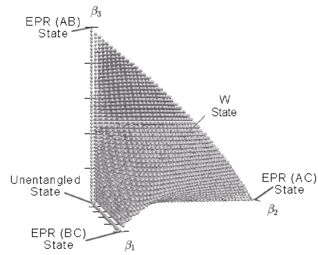
Figure 1: Entanglement types for $\beta_{4}=0$.

Next we consider the entanglement possibilities for a fixed value of $\beta_{4}$ in the range $0<\beta_{4}<1/4$. In this case, the conditions of Proposition 2 produce the following allowable values of $\beta_{1}$, $\beta_{2}$, $\beta_{3}$.

$$\beta_{1}\geq 0,\hskip 14.22636pt\beta_{2}\geq 0,\hskip 14.22636pt\beta_{3}\geq 0$$ (36)

$$F\equiv\beta_{4}\left(\frac{1}{4}-\beta_{4}\right)+\sqrt{\beta_{1}\beta_{2}\beta_{3}}-\beta_{1}\beta_{2}-\beta_{1}\beta_{3}-\beta_{2}\beta_{3}\\ -(\beta_{1}+\beta_{2}+\beta_{3})\beta_{4}\geq 0$$ (37)

This region in $\beta_{1}$,$\beta_{2}$,$\beta_{3}$ space is a deformed tetrahedron bounded by four surfaces, as shown in Figure 2. For points on the boundary of the tetrahedron, conditions (19) and (20) uniquely determine values for $\beta_{5}$ and $\beta_{6}$ from the values of $\beta_{1}$, $\beta_{2}$, and $\beta_{3}$. For points in the interior of the tetrahedron, conditions (19) and (20) give the allowable values for $\beta_{5}$ and $\beta_{6}$ as a deformed circle, shown in Figure 3.

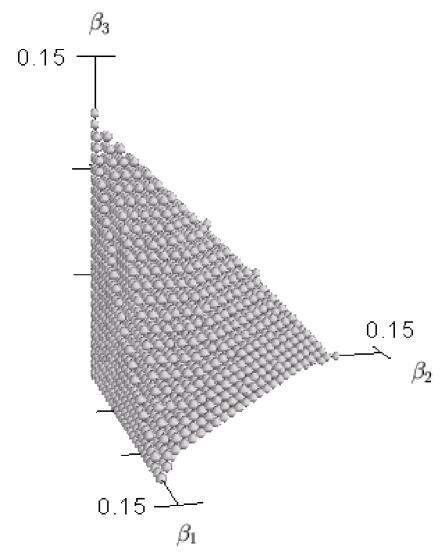
Figure 2: Entanglement possibilities for $\beta_{4}=1/8$. Each point in the interior of the deformed tetrahedron has a circle of entanglement types in the $\beta_{5}$,$\beta_{6}$ plane, as shown in Figure 3. Each point on the boundary of the tetrahedron represents a single entanglement type.

Figure 3: Each point on this deformed circle is an entanglement type with $\beta_{4}=1/8$, $\beta_{1}=\beta_{2}=\beta_{3}=0.03$. Every point in the interior of the deformed tetrahedron of Figure 2 has a circle of entanglement types like this. Points on the boundary of Figure 2 have a single entanglement type.

Finally, let us consider entanglement types for which $\beta_{4}=1/4$. In this case, conditions (19) and (22) lead to requirements that can only be satisfied if $\beta_{1}=\beta_{2}=\beta_{3}=\beta_{5}=\beta_{6}=0$. Thus, there is just a single type of entanglement with $\beta_{4}=1/4$, and it is the entanglement type of the GHZ state.

Table 2 classifies three-qubit entanglement types in a topological way, viewing $\mathcal{E}_{3}$ as a 5-dimensional cell complex. Each entanglement type belongs to exactly one cell (one row of the table). In addition to listing the ranges of the invariants for each cell of entanglement types, we also give the classification of Acín et al., the SLOCC class, and the orbit dimension for entanglement types in each cell.

Acín et al. classified entanglement for pure three-qubit states in Acín et al. (2000). Their classification was based on the number of basis states in (8) required to express a standard state with a particular entanglement type. In Table 2, we list the Acín type from Acín et al. (2000) associated with each cell of LU entanglement types.

The fourth column of Table 2 lists the SLOCC class for each cell of LU entanglement types. In the case of pure three-qubit states, the number of SLOCC entanglement types is finite: there are six Dür et al. (2000).

In addition to the classification scheme of Acín and the classification based on SLOCC, entanglement types can be classified by the dimension of their local unitary orbits. Each LU orbit is a differentiable manifold with a well-defined dimension. Carteret and Sudbery found the orbit dimensions for three-qubit pure states in Carteret and Sudbery (2000). The analysis of orbit dimensions appears to be a promising route toward classification of $n$-qubit states Lyons and Walck (a, b). In the last column of Table 2, we give the orbit dimension calculated for entanglement types in each cell.

Table 2: Three-qubit space of entanglement types viewed as a cell complex. The superscript in the cell name gives the dimension of the cell. The function $F$ is defined in (37).

Cell	Invariant	Acín	SLOCC	Orbit
name	ranges	Type Acín et al. (2000)	Class Dür et al. (2000)	Dimension
	$\beta_{4}=0$ (consequently $\beta_{5}=2\sqrt{\beta_{1}\beta_{2}\beta_{3}}$, $\beta_{6}=0$)
$e^{0}_{A-B-C}$	$\beta_{1}=\beta_{2}=\beta_{3}=0$	1	$A-B-C$	6
$e^{1}_{A-BC}$	$0<\beta_{1}<1/4$, $\beta_{2}=\beta_{3}=0$	2a	$A-BC$	7
$e^{0}_{A-BC}$	$\beta_{1}=1/4$, $\beta_{2}=\beta_{3}=0$	2a	$A-BC$	5
$e^{1}_{B-AC}$	$0<\beta_{2}<1/4$, $\beta_{1}=\beta_{3}=0$	2a	$B-AC$	7
$e^{0}_{B-AC}$	$\beta_{2}=1/4$, $\beta_{1}=\beta_{3}=0$	2a	$B-AC$	5
$e^{1}_{C-AB}$	$0<\beta_{3}<1/4$, $\beta_{1}=\beta_{2}=0$	2a	$C-AB$	7
$e^{0}_{C-AB}$	$\beta_{3}=1/4$, $\beta_{1}=\beta_{2}=0$	2a	$C-AB$	5
$e^{3}_{W}$	$0<\beta_{1}\beta_{2}+\beta_{1}\beta_{3}+\beta_{2}\beta_{3}<\sqrt{\beta_{1}\beta_{2}\beta_{3}}$	4a	$W$	9
$e^{2}_{W}$	$0<\beta_{1}\beta_{2}+\beta_{1}\beta_{3}+\beta_{2}\beta_{3}=\sqrt{\beta_{1}\beta_{2}\beta_{3}}$	3a	$W$	8
	$0<\beta_{4}<1/4$
$e^{1}_{GHZ}$	$\beta_{1}=\beta_{2}=\beta_{3}=0$	2b	$GHZ$	7
$e^{1}_{A,GHZ}$	$\beta_{1}=1/4-\beta_{4}$, $\beta_{2}=\beta_{3}=0$	3b	$GHZ$	8
$e^{1}_{B,GHZ}$	$\beta_{2}=1/4-\beta_{4}$, $\beta_{1}=\beta_{3}=0$	3b	$GHZ$	8
$e^{1}_{C,GHZ}$	$\beta_{3}=1/4-\beta_{4}$, $\beta_{1}=\beta_{2}=0$	3b	$GHZ$	8
$e^{2}_{A,GHZ}$	$0<\beta_{1}<1/4-\beta_{4}$, $\beta_{2}=\beta_{3}=0$	3b	$GHZ$	8
$e^{2}_{B,GHZ}$	$0<\beta_{2}<1/4-\beta_{4}$, $\beta_{1}=\beta_{3}=0$	3b	$GHZ$	8
$e^{2}_{C,GHZ}$	$0<\beta_{3}<1/4-\beta_{4}$, $\beta_{1}=\beta_{2}=0$	3b	$GHZ$	8
$e^{2}_{BC}$	$\beta_{1}=0$, $\beta_{2}\beta_{3}>0$, $F=0$	5	$GHZ$	9
$e^{2}_{AC}$	$\beta_{2}=0$, $\beta_{1}\beta_{3}>0$, $F=0$	4b	$GHZ$	9
$e^{2}_{AB}$	$\beta_{3}=0$, $\beta_{1}\beta_{2}>0$, $F=0$	4b	$GHZ$	9
$e^{3}_{BC}$	$\beta_{1}=0$, $\beta_{2}\beta_{3}>0$, $F>0$	5	$GHZ$	9
$e^{3}_{AC}$	$\beta_{2}=0$, $\beta_{1}\beta_{3}>0$, $F>0$	4b	$GHZ$	9
$e^{3}_{AB}$	$\beta_{3}=0$, $\beta_{1}\beta_{2}>0$, $F>0$	4b	$GHZ$	9
$e^{3}_{ABC}$	$\beta_{1}\beta_{2}\beta_{3}>0$, $F=0$	5	$GHZ$	9
$e^{4}$	$\beta_{1}\beta_{2}\beta_{3}>0$, $F>0$, $\beta_{5}=2\sqrt{\beta_{1}\beta_{2}\beta_{3}}$	5	$GHZ$	9
$e^{5}$	$\beta_{1}\beta_{2}\beta_{3}>0$, $F>0$, $\beta_{5}<2\sqrt{\beta_{1}\beta_{2}\beta_{3}}$	5	$GHZ$	9
	$\beta_{4}=1/4$
$e^{0}_{GHZ}$	(consequently $\beta_{1}=\beta_{2}=\beta_{3}=\beta_{5}=\beta_{6}=0$)	2b	$GHZ$	7

VI Topology and Standard States

The Schmidt decomposition theorem provides a set of standard quantum states and a claim that every bipartite quantum state is LU equivalent to one of the standard states. Various generalizations of the Schmidt decomposition to multipartite systems have been proposed Acín et al. (2000); Carteret et al. (2000). Standard states, such as (8), have been invaluable in understanding three-qubit entanglement. The two-qubit Schmidt decomposition theorem, which states that every two-qubit state is LU-equivalent to a state of the form $\alpha_{1}\left|00\right\rangle+\alpha_{2}\left|11\right\rangle$, with $\alpha_{1}$ and $\alpha_{2}$ real, $\alpha_{1}\geq\alpha_{2}$, and $\alpha_{1}^{2}+\alpha_{2}^{2}=1$, is particularly nice in that it provides

• exactly one standard state for each LU entanglement type, and

• standard states that are close together when their entanglement types are close together.

Generalizations of the Schmidt decomposition to three qubits or more have not been able to retain both of these properties. This naturally leads to the question of whether a nice set of three-qubit standard states exists, and has yet to be found, or does not exist.

We use topological properties of $\mathcal{E}_{3}$ to argue that no nice set of standard states exists for three qubits. We can translate the two nice properties above into mathematical requirements. The first property, that each entanglement type have a unique standard state, is imposed by requiring a map from the space of entanglement types to the space of quantum states. For three qubits, we need a map $\sigma:\mathcal{E}_{3}\to\mathbb{CP}^{7}$. The second property, that entanglement types that are close have standard states that are close, is satisfied by requiring that the map $\sigma$ be continuous.

Recall that we already have a continuous projection map $\pi:\mathbb{CP}^{7}\to\mathcal{E}_{3}$. The composition of these two, $\pi\circ\sigma$, must be the identity map on $\mathcal{E}_{3}$.

$$\mathcal{E}_{3}\xrightarrow{\sigma}\mathbb{CP}^{7}\xrightarrow{\pi}\mathcal{E}_{3}$$

Continuous maps between topological spaces induce homomorphisms between the associated homology groups. We will argue below that $\mathcal{E}_{3}$ has the homotopy type of $S^{5}$, in which case the homology group $H_{5}(\mathcal{E}_{3})=H_{5}(S^{5})$ is not trivial. On the other hand, $H_{5}(\mathbb{CP}^{7})$ and $H_{5}(S^{15})$ are trivial Hatcher (2002). If there were a continuous map $\sigma:\mathcal{E}_{3}\to\mathbb{CP}^{7}$, then in the composition of homomorphisms

$$H_{5}(\mathcal{E}_{3})\xrightarrow{\sigma_{*}}H_{5}(\mathbb{CP}^{7})\xrightarrow{\pi_{*}}H_{5}(\mathcal{E}_{3}),$$

$\pi_{*}\circ\sigma_{*}$ must be the identity map on $H_{5}(\mathcal{E}_{3})$. But this is impossible, since $H_{5}(\mathbb{CP}^{7})$ is trivial. It follows that there is no continuous map $\sigma:\mathcal{E}_{3}\to\mathbb{CP}^{7}$ such that $\pi\circ\sigma$ is the identity map on $\mathcal{E}_{3}$. Hence there is no set of three-qubit standard states with the two nice properties above.

It remains to argue that $\mathcal{E}_{3}$ has the homotopy type of $S^{5}$. For a fixed value of $\beta_{4}$ in the range $0<\beta_{4}<1/4$, in Section V we found a deformed tetrahedron of possible values of $(\beta_{1},\beta_{2},\beta_{3})$, with an additional circle of possibilities for $(\beta_{5},\beta_{6})$ when $(\beta_{1},\beta_{2},\beta_{3})$ was in the interior of the tetrahedron. A tetrahedron is homeomorphic to a ball $D^{3}=\{(x,y,z)\in\mathbb{R}^{3}|x^{2}+y^{2}+z^{2}\leq 1\}$. The additional circle of possibilities in the interior of the ball, but not on the boundary of the ball implies that the entire space of entanglement types with a fixed $\beta_{4}$ is homeomorphic to the quotient space of $D^{3}\times S^{1}$ in which $S^{1}$ collapses to a point on the boundary of $D^{3}$. The space of entanglement types with a fixed $\beta_{4}\in(0,1/4)$ is therefore homeomorphic to $S^{4}$. If this were the case for all values of $\beta_{4}$, including $0$ and $1/4$, then the space of entanglement types would look like $[0,1/4]\times S^{4}$. But we know that when $\beta_{4}=1/4$, the 4-sphere shrinks to a point, and when $\beta_{4}=0$, the 4-sphere collapses to $D^{3}$. We conclude that $\mathcal{E}_{3}$ is homeomorphic to the quotient space of $[0,1/4]\times S^{4}$ in which $S^{4}$ collapses to $D^{3}$ at the left endpoint of $[0,1/4]$, and $S^{4}$ collapses to a point at the right endpoint.

Now, $S^{5}$ is homeomorphic to the quotient space of $[0,1/4]\times S^{4}$ when $S^{4}$ shrinks to a point at both ends of $[0,1/4]$. The quotient map $\mathcal{E}_{3}\to S^{5}$ that collapses $D^{3}$ to a point is a homotopy equivalence since $(\mathcal{E}_{3},D^{3})$ is a CW pair (Hatcher, 2002, p. 11). We conclude that $\mathcal{E}_{3}$ and $S^{5}$ have the same homotopy type.

Note that $\mathcal{E}_{2}$, by comparison, has trivial topology (the closed interval $[0,1]$ is contractible), which explains why the two-qubit Schmidt decomposition can provide a nice set of standard states.

VII Acknowledgments

The authors thank Research Corporation for their support of this work. We also thank David Lyons for reading the manuscript.

References

- Linden and Popescu (1998) N. Linden and S. Popescu, Fortschr. Phys. 46, 567 (1998), e-print quant-ph/9711016.
- Hatcher (2002) A. Hatcher, Algebraic Topology (Cambridge University Press, 2002).
- Linden et al. (1999) N. Linden, S. Popescu, and A. Sudbery, Phys. Rev. Lett. 83, 243 (1999), e-print quant-ph/9801076.
- Kempe (1999) J. Kempe, Phys. Rev. A 60, 910 (1999), e-print quant-ph/9902036.
- Coffman et al. (2000) V. Coffman, J. Kundu, and W. K. Wootters, Phys. Rev. A 61, 052306 (2000), e-print quant-ph/9907047.
- Sudbery (2001) A. Sudbery, J. Phys. A 34, 643 (2001), e-print quant-ph/0001116.
- Acín et al. (2000) A. Acín, A. Andrianov, L. Costa, E. Jané, J. I. Latorre, and R. Tarrach, Phys. Rev. Lett. 85, 1560 (2000), e-print quant-ph/0003050.
- Acín et al. (2001) A. Acín, A. Andrianov, E. Jané, and R. Tarrach, J. Phys. A 34, 6725 (2001), e-print quant-ph/0009107.
- Munkres (2000) J. R. Munkres, Topology (Prentice Hall, 2000), 2nd ed.
- Hill and Wootters (1997) S. Hill and W. K. Wootters, Phys. Rev. Lett. 78, 5022 (1997).
- Ekert and Knight (1995) A. Ekert and P. L. Knight, Am. J. Phys. 63, 415 (1995).
- Aravind (1996) P. K. Aravind, Am. J. Phys. 64, 1143 (1996).
- Dür et al. (2000) W. Dür, G. Vidal, and J. I. Cirac, Phys. Rev. A 62, 062314 (2000), e-print quant-ph/0005115.
- Kuś and Życzkowski (2001) M. Kuś and K. Życzkowski, Phys. Rev. A 63, 032307 (2001), e-print quant-ph/0006068.
- (15) S. N. Walck, e-print quant-ph/0201111.
- Weyl (1939) H. Weyl, The Classical Groups: Their Invariants and Representations (Princeton University Press, 1939).
- Gingrich (2002) R. M. Gingrich, Phys. Rev. A 65, 052302 (2002).
- Carteret and Sudbery (2000) H. A. Carteret and A. Sudbery, J. Phys. A 33, 4981 (2000), e-print quant-ph/0001091.
- Lyons and Walck (a) D. W. Lyons and S. N. Walck, e-print quant-ph/0503052.
- Lyons and Walck (b) D. W. Lyons and S. N. Walck, e-print quant-ph/0506241.
- Carteret et al. (2000) H. A. Carteret, A. Higuchi, and A. Sudbery, J. Math. Phys. 41, 7932 (2000), e-print quant-ph/0006125.