Chapter

PhD Dissertation Institute of Nuclear Physics of Polish Academy of Sciences, Kraków
and
Université Pierre et Marie Curie, Paris

— To my parents —

Combinatorics of boson normal ordering
and some applications

Chapter 0 Preface

The subject of this thesis is the investigation of the combinatorial structures arising in the boson normal ordering problem. This research project arose from the collaboration between the Henryk Niewodniczański Institute of Nuclear of Polish Academy of Sciences in Cracow and Laboratoire de Physique Théorique de la Matière Condensée of the University of Pierre and Marie Curie in Paris.
The thesis was written under the common supervision of Prof. Karol A. Penson (LPTMC, Paris VI) and Prof. Edward Kapuścik (IFJ PAN, Cracow) under the program of co-tutelle. I am deeply grateful to them for the help and knowledge they have generously shared with me during my studies. My appreciation goes also to our collaborators Dr Andrzej Horzela (IFJ PAN, Cracow), Prof. Allan I. Solomon (Open University, UK) and Prof. Gerard Duchamp (LIPN, Paris XIII).
I have benefited a lot from discussions with Prof. Labib Haddad, Prof. Pinaki Roy, Prof. Mark Yor, Prof. Giuseppe Dattoli, Prof. Miguel A. Méndez, Prof. Cestmir Burdik, Prof. Krzysztof Kowalski and Dr. Jerzy Cislo.
I would also like to thank Prof. Bertrand Guillot, Prof. Ryszard Kerner from LPTMC (Paris VI) and Prof. Marek Kutschera, Prof. Wojciech Broniowski, Prof. Krzysztof Golec-Biernat, Prof. Wojciech Florkowski, Prof. Piotr Żenczykowski and Prof. Piotr Zieliński from IFJ PAN (Cracow) for their interest and warm support.
My utmost gratitude goes to my parents, to whom I dedicate this work.

Chapter 1 Introduction

In this work we are concerned with the one mode boson creation $a^{\dagger}$ and annihilation $a$ operators satisfying the commutation relation $[a,a^{\dagger}]=1$. We are interested in the combinatorial structures arising in the problem of normal ordering of a wide class of boson expressions. It shall provide us with the effective tools for systematic treatment of these problems.
By normal ordering of an operator expressed through the boson $a$ and $a^{\dagger}$ operators we mean moving all annihilation operators to the right of all creation operators with the use of commutation relation. This procedure yields an operator which is equivalent (in the operator sense) to the original one but has a different functional representation. It is of both mathematical and physical interest. From the mathematical point of view it allows one to represent the operator by a function of two, in a sense ’commuting’, variables. It is also connected with the physicist’s perspective of the problem. Commonly used, the so called coherent state representation (see Appendix 8) implicitly requires the knowledge of the normally ordered form of the operators in question. Put the other way, for the normally ordered operator its coherent state matrix elements may be immediately read off. This representation is widely used e.g. in quantum optics. We mention also that calculation of the vacuum expectation values is much easier for operators in the normally ordered form. For other applications see [KS85].
A standard approach to the normal ordering problem is through the Wick theorem. It directly links the problem to combinatorics, i.e. searching for all possible contractions in the boson expression and then summing up the resulting terms. This may be efficiently used for solving problems with finite number of boson operators (especially when one uses the computer algebra packages). Although this looks very simple in that form it is not very constructive in more sophisticated cases. The main disadvantage is that it does not give much help in solving problems concerning operators defined through infinite series expansions. To do this we would have to know the underlying structure of the numbers involved. This still requires a lot of careful analysis (not accessible to computers). In this work we approach these problems using methods of advanced combinatorial analysis [Com74]. It proves to be an efficient way for obtaining compact formulas for normally ordered expansion coefficients and then analyzing theirs properties.
A great body of work was already put in the field. In his seminal paper [Kat74] Jacob Katriel pointed out that the numbers which come up in the normal ordering problem for $(a^{\dagger}a)^{n}$ are the Stirling numbers of the second kind. Later on, the connection between the exponential generating function of the Bell polynomials and the coherent state matrix elements of $e^{\lambda a^{\dagger}a}$ was provided [Kat00][Kat02]. In Chapter 3 we give a modern review of these results with special emphasis on the Dobiński relations. We also make use of a specific realization of the commutation relation $[a,a^{\dagger}]=1$ in terms of the multiplication $X$ and derivative $D$ operators. It may be thought of as an introduction to the methods used later on in this text. Chapter 4 is written in that spirit. We use this methodology to investigate and obtain compact formulas for the coefficients arising in normal ordering of a boson monomial (string of boson creation and annihilation operators). Then we proceed to the normal ordering of powers of a boson string and more generally homogeneous boson polynomial (i.e. the combinations of the of the boson strings with the same excess of creation over annihilation operators). The numbers appearing in the solution generalize Stirling and Bell numbers of the second kind. For this problem we also supply the exponential generating functions which are connected with the exponentials of the operators in question. In each case we provide the coherent state matrix elements of the boson expressions.
Recalling the current state of the knowledge in the field we should also mention the approach based on Lie-group methodology [Wil67]. It proves useful for normal ordering problems for the exponentials of expressions which are quadratic in boson operators [Meh77][AM77].
In a series of papers by various authors [Wit75][Mik83][Mik85][Kat83] some effort in extending these results to operators having the specific form $(a^{\dagger}a+(a^{\dagger})^{r})^{n}$ was made. In Chapter 5 we systematically extend this class to operators of the form $(q(a^{\dagger})a+v(a^{\dagger}))^{n}$ and $e^{\lambda(q(a^{\dagger})a+v(a^{\dagger}))}$ where $q(x)$ and $v(x)$ are arbitrary functions. This is done by the use of umbral calculus methods [Rom84] in finding representations of the monomiality principle (i.e. representations of the Heisenberg-Weyl algebra in the space of polynomials) and application of the coherent state methodology. Moreover, we establish a one-to-one connection between this class of normal ordering problems and the family of Sheffer-type polynomials.
These two classes of problems extend the current state of knowledge on the subject in two different directions in a quite systematic way. We believe this to be a considerable push forward in the normal ordering problem. We also emphasize the use of combinatorial methods which we give explicitly and which prove to be very efficient in this kind of analysis.
We illustrate this approach by examples taken both from combinatorics and physics (e.g. for the hamiltonian of a generalized Kerr medium). Moreover we also comment on applications and extensions of the formalism. We give just a few of them in Chapter 6. First we observe how to extend this formalism to the case of deformed commutation relations. In general it can be done at the expense of introducing operator-valued Stirling numbers. Next, we use the fact that the use of the Dobiński relations allow us to find the solutions to the Stieltjes moment problem for the numbers arising in the normal ordering procedure. We use these solutions to construct and analyze new families of generalized coherent states [KS85]. We end by commenting on the specific form of the formulas obtained in Chapter 5 which may be used to derive the explicit action of generalized shift operators, called the substitution theorem. These three examples already show that the methods we use in solving normal ordering problems lead to many diverse applications. At the end this text we append complete list of publications which indicate some other developments on the subject.

Chapter 2 Preliminaries

  In this chapter we give basic notions exploited later on in the text. We start by fixing some conventions. Next we recall the occupation number representation along with the creation $a^{\dagger}$ and annihilation $a$ operator formalism. This serves to define and comment on the normal ordering problem for boson operators. We end by pointing out a particular representation of the above in terms of the multiplication and derivative operators.
 

1 Conventions

In the mathematical literature there is always a certain freedom in making basic definitions. Sometimes it is confusing, though. For that reason it is reasonable to establish explicitly some conventions in the beginning.
In the following by an indeterminate we primarily mean a formal variable in the context of formal power series (see Section 9). It may be thought as a real or complex number whenever the analytic properties are assured.
We frequently make use of summation and the product operations. We give the following conventions concerning their limits

$$\sum_{n=N_{0}}^{N}...=0\ \ \ \ \ \ \ \ \text{and}\ \ \ \ \ \ \ \ \prod_{n=N_{0}}^{N}...=1\ \ \ \ \ \ \ \ \ \ \ \ \text{for}\ \ N<N_{0}.$$

Also the convention $0^{0}=1$ is applied.
Moreover we define the so called falling factorial symbol by

$$x^{\underline{k}}=x\cdot(x-1)\cdot...\cdot(x-k+1),\ \ \ \ \ \ \ \ \ \ x^{\underline{0}}=1,$$

for nonnegative integer $k$ and indeterminate $x$.
By the ceiling function $\lceil x\rceil$, for $x$ real, we mean the nearest integer greater or equal to $x$.

2 Occupation number representation: Boson operators

We consider a pair of one mode boson annihilation $a$ and creation $a^{\dagger}$ operators satisfying the commutation relation

$$[a,a^{\dagger}]=1.$$ (1)

Together with the identity operator the generators $\{a,a^{\dagger},1\}$ constitute the Heisenberg-Weyl algebra.
The occupation number representation arises from the interpretation of $a$ and $a^{\dagger}$ as operators annihilating and creating a particle (object) in a system. From this point of view the Hilbert space $\mathcal{H}$ of states (sometimes called Fock space) is generated by the number states $|n\rangle$, where $n=0,1,2,...$ count the number of particles (for bosons up to infinity). We assume here the existence of a unique vacuum state $|0\rangle$ such that

$$a|0\rangle=0.$$ (2)

Then the number states $\{|n\rangle\}_{n=0}^{\infty}$ may be taken as an orthonormal basis in $\mathcal{H}$, i.e.

$$\langle n|k\rangle=\delta_{n,k}$$ (3)

and

$$\sum_{n=0}^{\infty}|n\rangle\langle n|=1.$$ (4)

The last operator equality is called a resolution of unity which is equivalent to the completeness property.
It may be deduced from Eqs.(1) and (2) that operators $a$ and $a^{\dagger}$ act on the number states as

$$\begin{array}[]{rcr}a\ |n\rangle&=&\sqrt{n}\ |n-1\rangle,\\ a^{\dagger}|n\rangle&=&\sqrt{n+1}\ |n+1\rangle.\end{array}$$ (7)

(Indetermined phase factors may be incorporated into the states.)
Then all states may be created from the vacuum through

$$|n\rangle=\frac{1}{\sqrt{n!}}(a^{\dagger})^{n}|0\rangle.$$ (8)

It also follows that the number operator $N$ counting the number of particles in a system and defined by

$$N|n\rangle=n|n\rangle$$ (9)

may be represented as $N=a^{\dagger}a$ and satisfies the the following commutation relations

$$\begin{array}[]{l}{[a,N]}=a,\\ {[a^{\dagger},N]}=-a^{\dagger}.\end{array}$$ (12)

This construction may be easily extended to the multi-boson case.
The canonical form of the commutator Eq.(1) originates from the study of a quantum particle in the harmonic oscillator potential and quantization of the electromagnetic field. Any standard textbook on Quantum Mechanics may serve to survey of these topics.
We note that the commutation relations of Eqs.(1) and (12) may be easily extended to the deformed case [Sol94] (see also Section 1).

3 Normal ordering

The boson creation $a^{\dagger}$ and annihilation $a$ operators considered in previous section do not commute. This is the reason for some ambiguities in the definitions of the operator functions in Quantum Mechanics. To solve this problem one has to additionally define the order of the operators involved.
These difficulties with operator ordering led to the definition of the normally ordered form of the boson operator in which all the creation operators $a^{\dagger}$ stand to the left of the annihilation operators $a$.
There are two well defined procedures on the boson expressions yielding a normally ordered form. Namely, the normal ordering $\mathcal{N}$ and the double dot $:\ :$ operations.
By normal ordering of a general function $F(a,a^{{\dagger}})$ we mean ${\cal N}\left[F(a,a^{{\dagger}})\right]$ which is obtained by moving all the annihilation operators $a$ to the right using the commutation relation of Eq.(1). We stress the fact that after this normal ordering procedure, the operator remains the same ${\cal N}\left[F(a,a^{{\dagger}})\right]=F(a,a^{{\dagger}})$. It is only its functional representation which changes.
On the contrary the double dot operation operation $:\!F(a,a^{{\dagger}})\!:$ means the same procedure but without taking into account the commutation relation of Eq.(1), i.e. moving all annihilation operators $a$ to the right as if they commute with the creation operators $a^{\dagger}$. We emphasize that in general $F(a,a^{{\dagger}})\neq\ :\!F(a,a^{{\dagger}})\!:$ . The equality holds only for operators which are already in normal form (e.g. ${\cal N}\left[F(a,a^{{\dagger}})\right]=\ :{\cal N}\left[F(a,a^{{\dagger}})\right]:$ ).
Using these two operations we say that the normal ordering problem for $F(a,a^{{\dagger}})$ is solved if we are able to find an operator $G(a,a^{{\dagger}})$ for which the following equality is satisfied

$$F(a,a^{{\dagger}})={\cal N}\left[F(a,a^{{\dagger}})\right]\equiv\ :G(a,a^{{\dagger}}):\ .$$ (13)

This normally ordered form is especially useful in the coherent state representation widely used in quantum optics (see Appendix 8). Also calculation of the vacuum expectation values in quantum field theory is immediate whenever this form is known.
Here is an example of the above ordering procedures

$$\begin{array}[]{rcc}aa^{\dagger}aaa^{\dagger}a&\xrightarrow[\ \ \ \ \ {[a,a^{\dagger}]=1}\ \ \ \ \ ]{\cal{N}}&\underbrace{(a^{\dagger})^{2}a^{4}+4\ a^{\dagger}a^{3}+2\ a^{2}}\vspace{2mm}\\ &&\footnotesize{a^{\dagger}\ \text{- to the left}\ \ \ a\ \text{- to the right}\vspace{2mm}}\\ aa^{\dagger}aaa^{\dagger}a&\xrightarrow[\scriptsize\begin{array}[]{c}a,a^{\dagger}\ \text{- commute}\\ \text{(like numbers)}\end{array}]{:\ \ :}&\overbrace{a^{\dagger}a^{\dagger}aaa}\end{array}$$ (19)

Another simple illustration is the ordering of the product $a^{k}(a^{\dagger})^{l}$ which is in the so called anti-normal form (i.e. all annihilation operators stand to the left of creation operators). The double dot operation readily gives

$$:a^{k}(a^{\dagger})^{l}:\ =(a^{\dagger})^{l}a^{k},$$

while the normal ordering procedure $\cal{N}$ requires some exercise in the use of Eq.(1) yielding (proof by induction)

$$a^{k}(a^{\dagger})^{l}={\cal N}\left[a^{k}(a^{\dagger})^{l}\right]\equiv\sum_{p=0}^{k}\binom{k}{p}l^{\underline{p}}\ (a^{\dagger})^{l-p}a^{k-p}.$$ (20)

These examples explicitly show that these two procedures furnish completely different results (except for the operators which are already in normal form).
There is also a ’practical’ difference in their use. That is while the application of the double dot operation $:\ :$ is almost immediate, for the normal ordering procedure $\cal{N}$ certain skill in commuting operators $a$ and $a^{\dagger}$ is needed.
A standard approach to the problem is by the Wick theorem. It reduces the normal ordering procedure $\cal{N}$ to the double dot operation on the sum over all possible contractions (contraction means removal of a pair of annihilation and creation operators in the expression such that $a$ precedes $a^{\dagger}$). Here is an example

$$aa^{\dagger}aaa^{\dagger}aaa^{\dagger} = \sum\ :\{\ \text{all contractions}\ \}:$$

$$= :aa^{\dagger}aaa^{\dagger}aaa^{\dagger}:$$

$$+:aa^{\dagger}aaa^{\dagger}a\not\!a\not\!a^{\dagger}+aa^{\dagger}aaa^{\dagger}\not\!aa\not\!a^{\dagger}+aa^{\dagger}a\not\!aa^{\dagger}aa\not\!a^{\dagger}+$$

$$\ \ \ \ \ aa^{\dagger}\not\!aaa^{\dagger}aa\not\!a^{\dagger}+\not\!aa^{\dagger}aaa^{\dagger}aa\not\!a^{\dagger}+aa^{\dagger}a\not\!a\not\!a^{\dagger}aaa^{\dagger}+$$

$$\ \ \ \ \ aa^{\dagger}\not\!aa\not\!a^{\dagger}aaa^{\dagger}+\not\!aa^{\dagger}aa\not\!a^{\dagger}aaa^{\dagger}+\not\!a\not\!a^{\dagger}aaa^{\dagger}aaa^{\dagger}:$$

$$+:aa^{\dagger}a\not\!a\not\!a^{\dagger}a\not\!a\not\!a^{\dagger}+aa^{\dagger}\not\!aa\not\!a^{\dagger}a\not\!a\not\!a^{\dagger}+\not\!aa^{\dagger}aa\not\!a^{\dagger}a\not\!a\not\!a^{\dagger}+$$

$$\ \ \ \ \ \not\!a\not\!a^{\dagger}aaa^{\dagger}a\not\!a\not\!a^{\dagger}+aa^{\dagger}a\not\!a\not\!a^{\dagger}\not\!aa\not\!a^{\dagger}+aa^{\dagger}\not\!aa\not\!a^{\dagger}\not\!aa\not\!a^{\dagger}+$$

$$\ \ \ \ \ \not\!aa^{\dagger}aa\not\!a^{\dagger}\not\!aa\not\!a^{\dagger}+\not\!a\not\!a^{\dagger}aaa^{\dagger}\not\!aa\not\!a^{\dagger}+aa^{\dagger}\not\!a\not\!a\not\!a^{\dagger}aa\not\!a^{\dagger}+$$

$$\ \ \ \ \ \not\!aa^{\dagger}a\not\!a\not\!a^{\dagger}aa\not\!a^{\dagger}+\not\!a\not\!a^{\dagger}a\not\!aa^{\dagger}aa\not\!a^{\dagger}+aa^{\dagger}\not\!a\not\!a\not\!a^{\dagger}aa\not\!a^{\dagger}+$$

$$\ \ \ \ \ \not\!aa^{\dagger}\not\!aa\not\!a^{\dagger}aa\not\!a^{\dagger}+\not\!a\not\!a^{\dagger}\not\!aaa^{\dagger}aa\not\!a^{\dagger}+\not\!aa^{\dagger}a\not\!a\not\!a^{\dagger}aa\not\!a^{\dagger}+$$

$$\ \ \ \ \ \not\!aa^{\dagger}\not\!aa\not\!a^{\dagger}aa\not\!a^{\dagger}+\not\!a\not\!a^{\dagger}a\not\!a\not\!a^{\dagger}aaa^{\dagger}+\not\!a\not\!a^{\dagger}\not\!aa\not\!a^{\dagger}aaa^{\dagger}:$$

$$+:\ \not\!a\not\!a^{\dagger}a\not\!a\not\!a^{\dagger}a\not\!a\not\!a^{\dagger}+\not\!a\not\!a^{\dagger}\not\!aa\not\!a^{\dagger}a\not\!a\not\!a^{\dagger}+\not\!a\not\!a^{\dagger}a\not\!a\not\!a^{\dagger}\not\!aa\not\!a^{\dagger}+$$

$$\ \ \ \ \ \not\!a\not\!a^{\dagger}\not\!aa\not\!a^{\dagger}\not\!aa\not\!a^{\dagger}+\not\!a\not\!a^{\dagger}\not\!a\not\!a\not\!a^{\dagger}aa\not\!a^{\dagger}+\not\!a\not\!a^{\dagger}\not\!a\not\!a\not\!a^{\dagger}aa\not\!a^{\dagger}:$$

$$= (a^{\dagger})^{3}a^{5}+9\ (a^{\dagger})^{2}a^{4}+18\ a^{\dagger}a^{3}+6\ a^{2}.$$

One can easily see that the number of contractions may be quite big. This difficulty for polynomial expressions may be overcome by using modern computer algebra systems. Nevertheless, for nontrivial functions (having infinite expansions) the problem remains open. Also it does not provide the analytic formulas for the coefficients of the normally ordered terms in the final expression. A systematic treatment of a large class of such problems is the subject of this work.
At the end of this Section we recall some formulas connected with operator reordering. The first one is the exponential mapping formula, sometimes called the Hausdorff transform, which for any well defined function $F(a,a^{\dagger})$ yields

$$\begin{array}[]{rcl}e^{xa}F(a,a^{\dagger})e^{-xa}&=&F(a,a^{\dagger}+x),\vspace{2mm}\\ e^{-xa^{\dagger}}F(a,a^{\dagger})e^{xa^{\dagger}}&=&F(a+x,a^{\dagger}).\end{array}$$ (23)

It can be used to derive the following commutators

$$\begin{array}[]{rcl}{[a,F(a,a^{\dagger})]}&=&\frac{\displaystyle\partial}{\displaystyle\partial a^{\dagger}}\ F(a,a^{\dagger}),\vspace{2mm}\\ {[a^{\dagger},F(a,a^{\dagger})]}&=&-\frac{\displaystyle\partial}{\displaystyle\partial a}\ F(a,a^{\dagger}).\end{array}$$ (26)

The proofs may be found in any book on Quantum Mechanics, e.g. [Lou64].
Also a well known property of the Heisenberg-Weyl algebra of Eq.(1) is a disentangling formula

$$e^{\lambda(a+a^{\dagger})}=e^{\lambda^{2}/2}e^{\lambda a^{\dagger}}e^{\lambda a}=e^{-\lambda^{2}/2}e^{\lambda a}e^{\lambda a^{\dagger}},$$ (27)

which may serve as an example of the normal ordering procedure

$$e^{\lambda(a+a^{\dagger})}={\cal{N}}\left[e^{\lambda(a+a^{\dagger})}\right]\equiv\ e^{\lambda^{2}/2}\ :e^{\lambda(a+a^{\dagger})}:\ .$$ (28)

This type of expressions exploits the Lie structure of the algebra and uses a simplified form of Baker-Campbell-Hausdorff formula. For this and other disentangling properties of the exponential operators, see [Wil67][Wit75][MSI93][Das96].
Finally, we must mention other ordering procedures also used in physics, like the anti-normal or the Weyl (symmetric) ordered form. We note that there exist translation formulas between these expressions, see e.g. [CG69][ST79].

4 $X$ and $D$ representation

The choice of the representation of the algebra may be used to simplify the calculations. In the following we apply this, although, we note that with some effort one could also manage using solely the operator properties of $a$ and $a^{\dagger}$.
There are some common choices of the Heisenberg-Weyl algebra representation in Quantum Mechanics. One may take e.g. a pair of hermitian operators $X$ and $P=i\frac{d}{dx}$ acting on the dense subspace of square integrable functions or the infinite matrix representation of Eq.(7) defined in the Fock space. This choice is connected with a particular interpretation intimately connected with the quantum mechanical problem to be solved.
Here we choose the simplest possible representation of the commutation relation of Eq.(1) which acts in the space of (formal) polynomials. We make the identification

$$\begin{array}[]{ccc}a^{\dagger}&\longleftrightarrow&X\\ a&\longleftrightarrow&D,\end{array}$$ (31)

where $X$ and $D$ are formal multiplication and derivative ($D=\frac{d}{dx}$) operators, respectively. They are defined by their action on monomials

$$\begin{array}[]{lcl}Xx^{n}&=&x^{n+1},\\ Dx^{n}&=&nx^{n-1}.\end{array}$$ (34)

(It also defines the action of these operators on the formal power series.)
Note that the commutation relation of Eq. (1) remains the same, i.e.

$$[D,X]=1.$$ (35)

For more details see Appendix 9 and Chapter 5.
This choice of representation is most appropriate, as we note that the problem we shall be concerned with has a purely algebraic background. We are interested in the reordering of operators, and that only depends on the algebraic properties of the commutator of Eqs.(1) or (35). We emphasize that the conjugacy property of the operators or the scalar product do not play any role in that problem. To get rid of these unnecessary constructions we choose the representation of the commutator of Eq.(1) in the space of polynomials defined by Eq.(34) where these properties do not play primary role, however possible to implement (see the Bargmann-Segal representation [Bar61][Seg63]). We benefit from this choice by the resulting increased simplicity of the calculations.

Chapter 3 Generic example. Stirling and Bell numbers.

  We define Stirling and Bell numbers as solutions to the normal ordering problem for powers and the exponential of the number operator $N=a^{\dagger}a$ , where $a$ and $a^{\dagger}$ are the annihilation and creation operators. All their combinatorial properties are derived using only this definition. Coherent state matrix elements of $N^{n}$ and $e^{\lambda N}$ are shown to be the Bell polynomials and their exponential generating function, respectively.
 

This Chapter may be thought of as a simple introduction to some methods and problems encountered later on in the text. We give a simple example on which all the essential techniques of the proceeding sections are used. Although Stirling and Bell numbers have a well established purely combinatorial origin [Com74][Rio84][Wil94][GKP94] we choose here a more physical approach. We define and investigate Stirling and Bell numbers as solutions to the normal ordering problem [Kat74][Kat00][Kat02].

Consider the number operator $N=a^{\dagger}a$ and search for the normally ordered form of its $n$-th power (iteration). It can be written as

$$\left(a^{\dagger}a\right)^{n}=\sum_{k=1}^{n}S(n,k)(a^{\dagger})^{k}a^{k}$$ (1)

where the integers $S(n,k)$ are the so called Stirling numbers.
One may also define the so called Bell polynomials

$$B(n,x)=\sum_{k=1}^{n}S(n,k)x^{k}$$ (2)

and Bell numbers

$$B(n)=B(n,1)=\sum_{k=1}^{n}S(n,k)$$ (3)

For convenience we apply the conventions

$$S(n,0) = \delta_{n,0}\ \ \ \ \ \text{and}\ \ \ \ \ \ S(n,k)=0\ \ \ \ \text{for}\ \ k>n$$ (4)

and

$$B(0)=B(0,x)=1.$$ (5)

(It makes the calculations easier, e.g. one may ignore the summation limits when changing their order.)
In the following we are concerned with the properties of these Stirling and Bell numbers.
First we state the recurrence relation for Stirling numbers

$$S(n+1,k)=kS(n,k)+S(n,k-1),$$ (6)

with initial conditions as in Eq.(4). The proof 9by induction) can be deduced from the equalities

$$\sum_{k=1}^{n+1}\ S(n+1,k)\ (a^{\dagger})^{k}a^{k}=\left(a^{\dagger}a\right)^{n+1}=a^{\dagger}a\left(a^{\dagger}a\right)^{n}$$

$$=\sum_{k=1}^{n}S(n,k)\ a^{\dagger}a(a^{\dagger})^{k}a^{k}\stackrel{{\scriptstyle(\ref{aa})}}{{=}}\sum_{k=1}^{n}S(n,k)\ (a^{\dagger})^{k}(a^{\dagger}a+k)a^{k}$$

$$=\sum_{k=2}^{n+1}S(n,k-1)\ (a^{\dagger})^{k}a^{k}+\sum_{k=1}^{n}k\ S(n,k)\ (a^{\dagger})^{k}a^{k}$$

$$\stackrel{{\scriptstyle(\ref{Initial})}}{{=}}\sum_{k=1}^{n+1}\left(S(n,k-1)+k\ S(n,k)\right)\ (a^{\dagger})^{k}a^{k}.$$

We shall not make make use of this recurrence relation, preferring the simpler analysis based on the Dobiński relation. To this end we proceed to the essential step which we shall extensively use later on, i.e. change of representation. Eq.(1) rewritten in the $X$ and $D$ representation (see Section 4) takes the form

$$\left(XD\right)^{n}=\sum_{k=1}^{n}S(n,k)\ X^{k}D^{k}.$$ (7)

With this trick we shall obtain all the properties of Stirling and Bell numbers.
We first act with this equation on the monomial $x^{m}$. This gives for $m$ integer

$$m^{n}=\sum_{k=1}^{n}S(n,k)m^{\underline{k}},$$

where $x^{\underline{k}}=x\cdot(x-1)\cdot...\cdot(x-k+1)$ is the falling factorial ($x^{\underline{0}}=1$). Observing that a (non zero) polynomial can have only a finite set of zeros justifies the generalization

$$x^{n}=\sum_{k=1}^{n}S(n,k)x^{\underline{k}}.$$ (8)

This equation can be interpreted as a change of basis in the space of polynomials. This gives an interpretation of Stirling numbers as the connection coefficients between two bases $\{x^{n}\}_{n=0}^{\infty}$ and $\{x^{\underline{n}}\}_{n=0}^{\infty}$.
Now we act with Eq.(7) on the exponential function $e^{x}$. We obtain

$$\sum_{k=0}^{\infty}k^{n}\frac{x^{k}}{k!}=e^{x}\sum_{k=1}^{n}S(n,k)x^{k}.$$

Recalling the definition of the Bell polynomials Eq.(2) we get

$$B(n,x)=e^{-x}\sum_{k=0}^{\infty}k^{n}\frac{x^{k}}{k!},$$ (9)

which is a celebrated Dobiński formula [Wil94]. It is usually stated for Bell numbers in the form

$$B(n)=\frac{1}{e}\sum_{k=1}^{\infty}\frac{k^{n}}{k!}.$$ (10)

Note that both series are convergent by the d’Alembert criterion.
The most striking property of the Dobiński formula is the fact that integer numbers $B(n)$ or polynomials $B(n,x)$ can be represented as nontrivial infinite sums. Here we only mention that this remarkable property provides also solutions to the moment problem (see Section 2)
In the following we shall exploit the Dobiński formula Eq.(9) to investigate further properties of Stirling and Bell numbers.
Applying the Cauchy multiplication rule Eq.(3) to Eq.(9) and comparing coefficients we obtain explicit expression for $S(n,k)$

$$S(n,k)=\frac{1}{k!}\sum_{j=1}^{k}\binom{k}{j}(-1)^{k-j}j^{n}.$$ (11)

Next, we define the exponential generating function of the polynomials $B(n,x)$ (see Appendix 9) as

$$G(\lambda,x)=\sum_{n=0}^{\infty}B(n,x)\frac{\lambda^{n}}{n!},$$ (12)

which contains all the information about the Bell polynomials. Substituting Eq.(9) into Eq.(12), changing the summation order and then identifying the expansions of the exponential functions we obtain

$$G(\lambda,x) = e^{-x}\sum_{n=0}^{\infty}\sum_{k=0}^{\infty}k^{n}\frac{x^{k}}{k!}\frac{\lambda^{n}}{n!}=e^{-x}\sum_{k=0}^{\infty}\frac{x^{k}}{k!}\sum_{n=0}^{\infty}k^{n}\frac{\lambda^{n}}{n!}$$

$$= e^{-x}\sum_{k=0}^{\infty}\frac{x^{k}}{k!}e^{\lambda k}=e^{-x}e^{xe^{\lambda}}.$$

Finally we may write the exponential generating function $G(\lambda,x)$ in the compact form

$$G(\lambda,x)=e^{x(e^{\lambda}-1)}.$$ (13)

Sometimes in applications the following exponential generating function of the Stirling numbers $S(n,k)$ is used

$$\sum_{n=k}^{\infty}S(n,k)\frac{\lambda^{n}}{n!}=\frac{(e^{\lambda}-1)^{k}}{k!}.$$ (14)

It can be derived by comparing expansions in $x$ of Eqs.(12) and (13)

$$G(\lambda,x) = 1+\sum_{n=1}^{\infty}\left(\sum_{k=1}^{n}S(n,k)x^{k}\right)\frac{\lambda^{n}}{n!}$$

$$= 1+\sum_{k=1}^{\infty}\left(\sum_{n=k}^{\infty}S(n,k)\frac{\lambda^{n}}{n!}\right)x^{k},$$

$$G(\lambda,x) = e^{x(e^{\lambda}-1)}=1+\sum_{k=1}^{\infty}\frac{(e^{\lambda}-1)^{k}}{k!}x^{k}.$$

Bell polynomials share an interesting property called the Sheffer identity (note resemblance to the binomial identity)

$$B(n,x+y)=\sum_{k=0}^{n}\binom{n}{k}B(k,y)B(n-k,x)$$ (15)

It is the consequence of the following equalities

$$\sum_{n=0}^{\infty}B(n,x+y)\frac{\lambda^{n}}{n!} = e^{(x+y)(e^{\lambda}-1)}=e^{x(e^{\lambda}-1)}e^{y(e^{\lambda}-1)}$$

$$= \sum_{n=0}^{\infty}B(n,x)\frac{\lambda^{n}}{n!}\cdot\sum_{n=0}^{\infty}B(n,y)\frac{\lambda^{n}}{n!}$$

$$\stackrel{{\scriptstyle(\ref{Cauchy})}}{{=}} \sum_{n=0}^{\infty}\left(\sum_{k=0}^{n}\binom{n}{k}B(k,y)B(n-k,x)\right)\frac{\lambda^{n}}{n!}.$$

By this identity and also by the characteristic exponential generating function of Eq.(13) Bell polynomials $B(n,x)$ are found to be of Sheffer-type (see Appendix 9).
Differentiating the exponential generating function of Eqs.(12) and (13) we have (see Eq.(5))

$$\sum_{n=0}^{\infty}B(n+1,x)\frac{\lambda^{n}}{n!}=\frac{\partial}{\partial\lambda}G(\lambda,x)=e^{\lambda}e^{x(e^{\lambda}-1)}=e^{\lambda}\sum_{n=0}^{\infty}B(n,x)\frac{\lambda^{n}}{n!}$$

which by the Cauchy product rule Eq.(3) yields the recurrence relation for the Bell polynomials

$$B(n+1,x)=\sum_{k=0}^{n}\binom{n}{k}B(k,x).$$ (16)

And consequently for the Bell numbers we have $B(n+1)=\sum_{k=0}^{n}\binom{n}{k}B(k)$.
By the same token applied to the exponential generating function of Stirling numbers $S(n,k)$ of Eq.(14) the recurrence relation of Eq.(6) can be also derived.
Finally, using any of the derived properties of Stirling or Bell numbers one can easily calculate them explicitly. Here are some of them

$$S(n,k),\ \ \ \ \ \ 1\leq k\leq n\qquad\qquad\qquad\qquad B(n)\ \ \$$

$$\begin{array}[]{cl|lllllllllllcc}\cline{3-14}\cr&&&&&&\\ n=1&&&1&&&&&&&&&&1&\\ n=2&&&1&1&&&&&&&&&2&\\ n=3&&&1&3&1&&&&&&&&5&\\ n=4&&&1&7&6&1&&&&&&&15&\\ n=5&&&1&15&25&10&1&&&&&&52&\\ n=6&&&1&31&90&65&15&1&&&&&203&\\ n=7&&&1&63&301&350&140&21&1&&&&877\\ n=8&&&1&127&966&1701&1050&266&28&1&&&4140\\ ...&&&...&...&...&...&...&...&...&...&...&&...\end{array}$$ (27)

Now we come back to normal ordering. Using the properties of coherent states (see Appendix 8) we conclude from Eqs.(1) and (2) that diagonal coherent state matrix elements generate Bell polynomials [Kat00]

$$\langle z|(a^{\dagger}a)^{n}|z\rangle=B(n,|z|^{2}).$$ (28)

Moreover, expanding the exponential $e^{\lambda a^{\dagger}a}$ and taking the diagonal coherent state matrix element we have

$$\langle z|e^{\lambda a^{\dagger}a}|z\rangle=\sum_{n=0}^{\infty}\langle z|(a^{\dagger}a)^{n}|z\rangle\frac{\lambda^{n}}{n!}=\sum_{n=0}^{\infty}B(n,|z|^{2})\frac{\lambda^{n}}{n!}.$$

We see that the diagonal coherent state matrix elements of $e^{\lambda a^{\dagger}a}$ yield the exponential generating function of the Bell polynomials (see Eqs.(12) and (13))

$$\langle z|e^{\lambda a^{\dagger}a}|z\rangle=e^{|z|^{2}(e^{\lambda}-1)}.$$ (29)

This result allows us to read off the normally ordered form of $e^{\lambda a^{\dagger}a}$ (see Appendix 8)

$$e^{\lambda a^{\dagger}a}={\cal N}\left[e^{\lambda a^{\dagger}a}\right]\equiv\ :e^{a^{\dagger}a(e^{\lambda}-1)}\ :.$$ (30)

These are more or less all properties of Stirling and Bell numbers. Note that they were defined here as solutions to the normal ordering problem for powers of the number operator $N=a^{\dagger}a$. The above analysis relied firmly on this definition.
On the other hand these numbers are well known in combinatorial analysis [Com74][Rio84][Wil94][GKP94] where are called Stirling numbers of the second kind and are usually explored using only recurrence relation Eq.(6). Here is their original interpretation is in terms of partitions of the set.

• Stirling numbers $S(n,k)$ count the number of ways of putting $n$ different objects into $k$ identical containers (none left empty).

• Bell numbers $B(n)$ count the number of ways of putting $n$ different objects into $n$ identical containers (some may be left empty).

Some other pictorial representations can be also given e.g. in terms of graphs [MBP05] or rook numbers [Nav73][SDB⁺04][Var04].

Chapter 4 Normal Ordering of Boson Expressions

  We solve the normal ordering problem for expressions in boson creation $a^{\dagger}$ and annihilation $a$ operators in the form of a string $(a^{\dagger})^{r_{M}}a^{s_{M}}\dots(a^{\dagger})^{r_{2}}a^{s_{2}}(a^{\dagger})^{r_{1}}a^{s_{1}}$. We are especially concerned with its powers (iterations). Next we extend the solution to iterated homogeneous boson polynomials, i.e. powers of the operators which are sums of boson strings of the same excess. The numbers obtained in the solutions are generalizations of Stirling and Bell numbers. Recurrence relations, closed-form expressions (including Dobiński-type relations) and generating formulas are derived. Normal ordering of the exponentials of the the aforementioned operators are also treated. Some special cases including Kerr-type hamiltonians are analyzed in detail.
 

1 Introduction

In this chapter we consider expressions in boson creation $a^{\dagger}$ and annihilation $a$ operators (see Section 2). We search for the normally ordered form and show effective ways of finding combinatorial numbers arising in that problem. These numbers generalize Stirling and Bell numbers (see Chapter 3).
The first class of expressions treated in this Chapter are so called boson strings or boson monomials, see Section 2. Here is an example

$$a^{\dagger}aa^{\dagger}a^{\dagger}aaa^{\dagger}a^{\dagger}a^{\dagger}a^{\dagger}a^{\dagger}aa^{\dagger}a^{\dagger}aaaaaaa^{\dagger}aa^{\dagger}aaa^{\dagger}a^{\dagger}a^{\dagger}aa^{\dagger},$$

which we compactly denote as

$$(a^{\dagger})^{r_{M}}a^{s_{M}}\dots(a^{\dagger})^{r_{2}}a^{s_{2}}(a^{\dagger})^{r_{1}}a^{s_{1}}$$

with some nonnegative integers $r_{m}$ and $s_{m}$. By an excess of a string we call the difference between the number of creation and annihilation operators, i.e. $d=\sum_{m=1}^{M}(r_{m}-s_{m})$. In the following we assume that the boson strings are of nonnegative excess (for negative excess see Section 6).
Boson strings (monomials) can be extended further to polynomials. We treat homogeneous boson polynomials which are combinations of boson monomials of the same excess (possibly with some coefficients). Here is an example

$$aaa^{\dagger}aa^{\dagger}a^{\dagger}aaa^{\dagger}a^{\dagger}a^{\dagger}+a^{\dagger}aa^{\dagger}a^{\dagger}a+a^{\dagger},$$

which using methods of Section 2 can be written in the form

$$(a^{\dagger})^{d}\ \sum_{k=N_{0}}^{N}\alpha_{k}\ (a^{\dagger})^{k}a^{k},$$

with appropriate $d$, $N$, $N_{0}$ and $\alpha_{k}$’s.
Next, in Sections 3 and 4 we give recipes on how to approach the problem of normal ordering of iterated boson strings and homogeneous boson polynomials, i.e. their $n$-th powers, like

$$\left(a^{\dagger}aa^{\dagger}a^{\dagger}aaa^{\dagger}a^{\dagger}a^{\dagger}a^{\dagger}a^{\dagger}aa^{\dagger}a^{\dagger}aaaaaaa^{\dagger}aa^{\dagger}aaa^{\dagger}a^{\dagger}a^{\dagger}aa^{\dagger}\right)^{n}$$

and

$$\left(aaa^{\dagger}aa^{\dagger}a^{\dagger}aaa^{\dagger}a^{\dagger}a^{\dagger}+a^{\dagger}aa^{\dagger}a^{\dagger}a+a^{\dagger}\right)^{n}.$$

These considerations serve to calculate in Section 5 the exponential generating functions of generalized Stirling and Bell numbers. This in turn gives the solution to the normal ordering problem of the exponential of the aforementioned boson operators.
In Section 6 we comment on operators with negative excess.
Finally in the last Section 7 we work out some examples which include generalized Kerr-type hamiltonian.
We refer to [MBP05][BPS⁺05][SDB⁺04][Var04] for interpretation of considered combinatorial structures in terms of graphs and rook polynomials.

2 General boson strings

In this section we define the generalization of ordinary Bell and Stirling numbers which arise in the solution of the general normal ordering problem for a boson string (monomial) [MBP05][Wit05]. Given two sequences of nonnegative integers ${\mathbf{r}}=(r_{1},r_{2},\dots,r_{M})$ and ${\mathbf{s}}=(s_{1},s_{2},\dots,s_{M})$ we define the operator

$$H_{{\mathbf{r}},{\mathbf{s}}}=(a^{\dagger})^{r_{M}}a^{s_{M}}\dots(a^{\dagger})^{r_{2}}a^{s_{2}}(a^{\dagger})^{r_{1}}a^{s_{1}}.$$ (1)

We let $S_{{\mathbf{r}},{\mathbf{s}}}(k)$ be the nonnegative integers appearing in the normally ordered expansion

$$H_{{\mathbf{r}},{\mathbf{s}}}=(a^{\dagger})^{d_{M}}\sum_{k=s_{1}}^{s_{1}+s_{2}+\dots+s_{M}}S_{{\mathbf{r}},{\mathbf{s}}}(k)(a^{\dagger})^{k}a^{k},$$ (2)

where $d_{n}=\sum_{m=1}^{n}(r_{m}-s_{m})$, $n=1,...,M$. Here we assume that the (overall) excess of a string is nonnegative $d_{M}\geq 0$ (for negative excess see Section 6).
Observe that the r.h.s. of Eq.(2) is already normally ordered and constitutes a homogeneous boson polynomial being the solution to the normal ordering problem. We shall provide explicit formulas for the coefficients $S_{{\mathbf{r}},{\mathbf{s}}}(k)$. This is a step further than the Wick’s theorem which is nonconstructive in that respect.
We call $S_{{\mathbf{r}},{\mathbf{s}}}(k)$ generalized Stirling number. The generalized Bell polynomial is defined as

$$B_{{\mathbf{r}},{\mathbf{s}}}(x)=\sum_{k=s_{1}}^{s_{1}+s_{2}+\dots+s_{M}}S_{{\mathbf{r}},{\mathbf{s}}}(k)x^{k},$$ (3)

and the generalized Bell number is the sum

$$B_{{\mathbf{r}},{\mathbf{s}}}=B_{{\mathbf{r}},{\mathbf{s}}}(1)=\sum_{k=s_{1}}^{s_{1}+s_{2}+\dots+s_{M}}S_{{\mathbf{r}},{\mathbf{s}}}(k).$$ (4)

Note that sequence of numbers $S_{{\mathbf{r}},{\mathbf{s}}}(k)$ is defined here for $s_{1}\leq k\leq s_{1}+s_{2}+\dots+s_{M}$. Initial terms may vanish (depending on the structure of ${\mathbf{r}}$ and ${\mathbf{s}}$), all the next are positive integers and the last one is equal to one, $S_{{\mathbf{r}},{\mathbf{s}}}(s_{1}+s_{2}+\dots+s_{M})=1$.
For convenience we apply the convention

$$S_{{\mathbf{r}},{\mathbf{s}}}(k)=0\ \ \ \ \ \ \ \ \ \text{for}\ \ k<s_{1}\ \ \text{or}\ \ k>s_{1}+s_{2}+\dots+s_{M}.$$ (5)

We introduce the notation ${\mathbf{r}}\ \uplus\ r_{M+1}=(r_{1},r_{2},\dots,r_{M},r_{M+1})$ and ${\mathbf{s}}\ \uplus\ s_{M+1}=(s_{1},s_{2},\dots,s_{M},s_{M+1})$ and state the recurrence relation satisfied by generalized Stirling numbers $S_{{\mathbf{r}},{\mathbf{s}}}(k)$

$$S_{{\mathbf{r}}\uplus r_{M+1},{\mathbf{s}}\uplus s_{M+1}}(k)=\sum_{j=0}^{s_{M+1}}\binom{s_{M+1}}{j}(d_{M}+k-j)^{\underline{s_{M+1}-j}}\ S_{{\mathbf{r}},{\mathbf{s}}}(k-j).$$ (6)

One can deduce the derivation of Eq.(6) from the following equalities

$$(a^{\dagger})^{d_{M+1}}\ \sum_{k=s_{1}}^{s_{1}+\dots+s_{M+1}}S_{{\mathbf{r}}\uplus r_{M+1},{\mathbf{s}}\uplus s_{M+1}}(k)\ (a^{\dagger})^{k}a^{k}$$

$$\stackrel{{\scriptstyle(\ref{SSS})}}{{=}}H_{{\mathbf{r}}\uplus r_{M+1},{\mathbf{s}}\uplus s_{M+1}}\stackrel{{\scriptstyle(\ref{hh})}}{{=}}(a^{\dagger})^{r_{M+1}}a^{s_{M+1}}H_{{\mathbf{r}},{\mathbf{s}}}$$

$$\stackrel{{\scriptstyle(\ref{SSS})}}{{=}}(a^{\dagger})^{r_{M+1}}a^{s_{M+1}}\ (a^{\dagger})^{d_{M}}\ \sum_{k=s_{1}}^{s_{1}+\dots+s_{M}}S_{{\mathbf{r}},{\mathbf{s}}}(k)\ (a^{\dagger})^{k}a^{k}$$

$$=(a^{\dagger})^{r_{M+1}}\ \sum_{k=s_{1}}^{s_{1}+\dots+s_{M}}S_{{\mathbf{r}},{\mathbf{s}}}(k)\ a^{s_{M+1}}(a^{\dagger})^{d_{M}+k}a^{k}$$

$$\stackrel{{\scriptstyle(\ref{aa})}}{{=}}(a^{\dagger})^{r_{M+1}}\ \sum_{k=s_{1}}^{s_{1}+\dots+s_{M}}S_{{\mathbf{r}},{\mathbf{s}}}(k)\ \sum_{j=0}^{s_{M+1}}\binom{s_{M+1}}{j}(d_{M}+k)^{\underline{j}}(a^{\dagger})^{d_{M}+k-j}a^{s_{M+1}+k-j}$$

$$=(a^{\dagger})^{d_{M+1}}\ \sum_{k=s_{1}}^{s_{1}+\dots+s_{M}}S_{{\mathbf{r}},{\mathbf{s}}}(k)\ \sum_{j=0}^{s_{M+1}}\binom{s_{M+1}}{j}(d_{M}+k)^{\underline{j}}(a^{\dagger})^{s_{M+1}+k-j}a^{s_{M+1}+k-j}$$

$$=(a^{\dagger})^{d_{M+1}}\ \sum_{j=0}^{s_{M+1}}\binom{s_{M+1}}{j}\sum_{k=s_{1}+s_{M+1}-j}^{s_{1}+\dots+s_{M+1}-j}S_{{\mathbf{r}},{\mathbf{s}}}(k)\ (d_{M}+k-s_{M+1}+j)^{\underline{j}}(a^{\dagger})^{k}a^{k}$$

$$\stackrel{{\scriptstyle(\ref{rec})}}{{=}}(a^{\dagger})^{d_{M+1}}\ \sum_{k=s_{1}}^{s_{1}\dots+s_{M}}\sum_{j=0}^{s_{M+1}}\binom{s_{M+1}}{j}S_{{\mathbf{r}},{\mathbf{s}}}(k-s_{M+1}+j)\ (d_{M}+k-s_{M+1}+j)^{\underline{j}}(a^{\dagger})^{k}a^{k}$$

$$=(a^{\dagger})^{d_{M+1}}\ \sum_{k=s_{1}}^{s_{1}+\dots+s_{M}}\sum_{j=0}^{s_{M+1}}\binom{s_{M+1}}{j}S_{{\mathbf{r}},{\mathbf{s}}}(k-j)\ (d_{M}+k-j)^{\underline{s_{M+1}-j}}(a^{\dagger})^{k}a^{k}$$

The problem stated in Eq.(2) can be also formulated in terms of multiplication $X$ and derivative $D$ operators (see Section 4)

$$X^{r_{M}}D^{s_{M}}\dots X^{r_{2}}D^{s_{2}}X^{r_{1}}D^{s_{1}}=X^{d_{M}}\sum_{k=s_{1}}^{s_{1}+s_{2}+\dots+s_{M}}\ S_{{\mathbf{r}},{\mathbf{s}}}(k)X^{k}D^{k}$$ (7)

Acting with the r.h.s. of Eq.(7) on the monomial $x^{l}$ we get $x^{l+d_{M}}\sum_{k=s_{1}}^{s_{1}+s_{2}+\dots+s_{M}}S_{{\mathbf{r}},{\mathbf{s}}}(k)l^{\underline{k}}$. On the other hand action of the l.h.s. on $x^{l}$ gives $\prod_{m=1}^{M}(d_{m-1}+l)^{\underline{s_{m}}}x^{l+d_{M}}$. Equating these two results (see Eq.(7)) we have

$$\prod_{m=1}^{M}(d_{m-1}+l)^{\underline{s_{m}}}=\sum_{k=s_{1}}^{s_{1}+s_{2}+\dots+s_{M}}S_{{\mathbf{r}},{\mathbf{s}}}(k)l^{\underline{k}}$$

By invoking the fact that the only polynomial with an infinite number of zeros is the zero polynomial we justify the generalization

$$\prod_{m=1}^{M}(d_{m-1}+x)^{\underline{s_{m}}}=\sum_{k=s_{1}}^{s_{1}+s_{2}+\dots+s_{M}}S_{{\mathbf{r}},{\mathbf{s}}}(k)x^{\underline{k}}.$$ (8)

This allows us to interpret the numbers $S_{{\mathbf{r}},{\mathbf{s}}}(k)$ as the expansion coefficients of the polynomial $\{\prod_{m=1}^{M}(d_{m-1}+x)^{\underline{s_{m}}}\}$ in the basis $\{x^{\underline{k}}\}_{k=0}^{\infty}$.
Now, replacing monomials in the above considerations with the exponential $e^{x}$ we conclude that

$$X^{r_{M}}D^{s_{M}}\dots X^{r_{2}}D^{s_{2}}X^{r_{1}}D^{s_{1}}\ e^{x} = x^{d_{M}}e^{x}B_{{\mathbf{r}},{\mathbf{s}}}(x)$$

$$X^{d_{M}}\sum_{k=s_{1}}^{s_{1}+s_{2}+\dots+s_{M}}S_{{\mathbf{r}},{\mathbf{s}}}(k)X^{k}D^{k}\ e^{x} = \sum_{k=s_{1}}^{\infty}\left[\prod_{m=1}^{M}(d_{m-1}+k)^{\underline{s_{m}}}\right]\frac{x^{k+d_{M}}}{k!}$$

With these two observations together and Eq.(7) we arrive at the Dobiński-type relation for the generalized Bell polynomial

$$B_{{\mathbf{r}},{\mathbf{s}}}(x)=e^{-x}\sum_{k=s_{1}}^{\infty}\left[\prod_{m=1}^{M}(d_{m-1}+k)^{\underline{s_{m}}}\right]\frac{x^{k}}{k!}$$ (9)

Observe that the d’Alembert criterion assures the convergence of the series.
Direct multiplication of series in Eq.(9) using the Cauchy rule of Eq.(3) gives the explicit formula for generalized Stirling numbers $S_{{\mathbf{r}},{\mathbf{s}}}(k)$

$$S_{{\mathbf{r}},{\mathbf{s}}}(k)=\frac{1}{k!}\sum_{j=0}^{k}\binom{k}{j}(-1)^{k-j}\prod_{m=1}^{M}(d_{m-1}+j)^{\underline{s_{m}}}\ .$$ (10)

We finally return to normal ordering and observe that the coherent state matrix element (see Appendix 8) of the boson string yields the generalized Bell polynomial (see Eqs.(1) and (2))

$$\langle z|H_{{\mathbf{r}},{\mathbf{s}}}|z\rangle=(z^{*})^{d_{M}}B_{{\mathbf{r}},{\mathbf{s}}}(|z|^{2}).$$ (11)

3 Iterated homogeneous polynomials in boson operators

Consider an operator $H_{\boldsymbol{\alpha}}^{d}$ of the form

$$H_{\boldsymbol{\alpha}}^{d}=(a^{\dagger})^{d}\ \sum_{k=N_{0}}^{N}\alpha_{k}\ (a^{\dagger})^{k}a^{k},$$ (12)

where the $\alpha_{k}$’s are constant coefficients (for convenience we take $\alpha_{N_{0}}\neq 0$ and $\alpha_{N}\neq 0$) and the nonnegative integer $d$ is the excess of the polynomial. Note that this is a homogeneous polynomial in boson operators. It is already in a normal form. If the starting homogeneous boson polynomial is not normally ordered then the methods of Section 2 provide proper tools to put it in the shape of Eq.(12). For boson polynomials of negative degree see Section 6.
Suppose we want to calculate the normally ordered form of $(H_{\boldsymbol{\alpha}}^{d})^{n}$. It can be written as

$$\left(H_{\boldsymbol{\alpha}}^{d}\right)^{n}=(a^{\dagger})^{nd}\ \sum_{k=N_{0}}^{nN}S_{\boldsymbol{\alpha}}^{d}(n,k)\ (a^{\dagger})^{k}a^{k},$$ (13)

with $S_{\boldsymbol{\alpha}}(n,k)$ to be determined. These coefficients generalize Stirling numbers (see Eq.(1)). In the same manner as in Eqs.(2) and (3) we define generalized Bell polynomials

$$B_{\boldsymbol{\alpha}}^{d}(n,x)=\sum_{k=N_{0}}^{nN}S_{\boldsymbol{\alpha}}^{d}(n,k)\ x^{k},$$ (14)

and generalized Bell numbers

$$B_{\boldsymbol{\alpha}}^{d}(n)=B_{\boldsymbol{\alpha}}^{d}(n,1)=\sum_{k=N_{0}}^{nN}S_{\boldsymbol{\alpha}}^{d}(n,k).$$ (15)

Note that $S_{{\mathbf{\alpha}}}^{d}(n,k)$, $B_{{\mathbf{\alpha}}}^{d}(n,x)$ and $B_{{\mathbf{\alpha}}}^{d}(n)$ depend on the set of $\alpha_{k}$’s defined in Eq.(12). For convenience we make the conventions

$$\begin{array}[]{ccl}S_{\boldsymbol{\alpha}}^{d}(0,0)&=&1,\\ S_{\boldsymbol{\alpha}}^{d}(n,k)&=&0\ \ \ \text{for}\ \ k>nN,\\ S_{\boldsymbol{\alpha}}^{d}(n,k)&=&0\ \ \ \text{for}\ \ k<N_{0}\ \ \text{and}\ \ n>0,\end{array}$$ (19)

and

$$B_{\boldsymbol{\alpha}}^{d}(0)=B_{\boldsymbol{\alpha}}^{d}(0,x)=1.$$ (20)

In the following we show how to calculate generalized Stirling and Bell numbers explicitly. First we state the recurrence relation

$$S_{\boldsymbol{\alpha}}^{d}(n+1,k)=\sum_{l=N_{0}}^{N}\alpha_{l}\ \sum_{p=0}^{l}\binom{l}{p}(nd+k-l+p)^{\underline{p}}\ S_{\boldsymbol{\alpha}}^{d}(n,k-l+p),$$ (21)

with initial conditions as in Eq.(19).
It can be deduced from the following equalities

$$(a^{\dagger})^{(n+1)d}\ \sum_{k=N_{0}}^{(n+1)N}S_{\boldsymbol{\alpha}}^{d}(n+1,k)\ (a^{\dagger})^{k}a^{k}\stackrel{{\scriptstyle(\ref{NHH})}}{{=}}(H_{\boldsymbol{\alpha}}^{d})^{n+1}=H_{\boldsymbol{\alpha}}(H_{\boldsymbol{\alpha}}^{d})^{n}$$

$$\stackrel{{\scriptstyle(\ref{NHH})}}{{=}}(a^{\dagger})^{d}\ \sum_{l=N_{0}}^{N}\alpha_{l}\ (a^{\dagger})^{l}a^{l}\ \ (a^{\dagger})^{nd}\ \sum_{k=N_{0}}^{nN}S_{\boldsymbol{\alpha}}^{d}(n,k)\ (a^{\dagger})^{k}a^{k}$$

$$=\sum_{k=N_{0}}^{nN}S_{\boldsymbol{\alpha}}^{d}(n,k)\sum_{l=N_{0}}^{N}\alpha_{l}\ (a^{\dagger})^{d+l}a^{l}\ (a^{\dagger})^{nd+k}a^{k}$$

$$\stackrel{{\scriptstyle(\ref{aa})}}{{=}}\sum_{k=N_{0}}^{nN}S_{\boldsymbol{\alpha}}^{d}(n,k)\sum_{l=N_{0}}^{N}\alpha_{l}\ (a^{\dagger})^{d+l}\left(\sum_{p=0}^{l}\binom{l}{p}(nd+k)^{\underline{p}}\ (a^{\dagger})^{nd+k-p}a^{l-p}\right)a^{k}$$

$$=(a^{\dagger})^{(n+1)d}\ \sum_{k=N_{0}}^{nN}S_{\boldsymbol{\alpha}}^{d}(n,k)\sum_{l=N_{0}}^{N}\alpha_{l}\ \sum_{p=0}^{l}\binom{l}{p}(nd+k)^{\underline{p}}\ (a^{\dagger})^{l+k-p}a^{l+k-p}$$

$$=(a^{\dagger})^{(n+1)d}\ \sum_{l=N_{0}}^{N}\alpha_{l}\ \sum_{p=0}^{l}\binom{l}{p}\sum_{k=N_{0}+l-p}^{nN+l-p}(nd+k-l+p)^{\underline{p}}\ S_{\boldsymbol{\alpha}}^{d}(n,k-l+p)(a^{\dagger})^{k}a^{k}$$

$$\stackrel{{\scriptstyle(\ref{InitialA})}}{{=}}(a^{\dagger})^{(n+1)d}\ \sum_{k=N_{0}}^{nN}\sum_{l=N_{0}}^{N}\alpha_{l}\ \sum_{p=0}^{l}\binom{l}{p}(nd+k-l+p)^{\underline{p}}\ S_{\boldsymbol{\alpha}}^{d}(n,k-l+p)(a^{\dagger})^{k}a^{k}.$$

Eq.(13) rewritten in the $X$ and $D$ representation takes the form

$$\left(H_{\boldsymbol{\alpha}}^{d}(D,X)\right)^{n}=X^{nd}\ \sum_{k=N_{0}}^{nN}S_{\boldsymbol{\alpha}}^{d}(n,k)\ X^{k}D^{k},$$ (22)

where

$$H_{\boldsymbol{\alpha}}^{d}(D,X)=X^{d}\ \sum_{k=N_{0}}^{N}\alpha_{k}\ X^{k}D^{k}.$$ (23)

We shall act with both sides of the Eq.(22) on the monomials $x^{l}$. The r.h.s. yields

$$X^{nd}\ \sum_{k=N_{0}}^{nN}S_{{\boldsymbol{\alpha}}}^{d}(n,k)\ X^{k}D^{k}\ x^{l}=\ \sum_{k=N_{0}}^{nN}S_{{\boldsymbol{\alpha}}}^{d}(n,k)\ l^{\underline{k}}x^{l+nd}.$$

On the other hand iterating the action of Eq.(23) on monomials $x^{l}$ we have

$$\left(H_{\boldsymbol{\alpha}}^{d}(D,X)\right)^{n}\ x^{l}=\left[\prod_{i=1}^{n}\sum_{k=N_{0}}^{N}\alpha_{k}\ (l+(i-1)d)^{\underline{k}}\right]x^{l+nd}.$$

Then when substituted in Eq.(22) we get

$$\prod_{i=1}^{n}\sum_{k=N_{0}}^{N}\alpha_{k}\ (l+(i-1)d)^{\underline{k}}=\ \sum_{k=N_{0}}^{nN}S_{{\boldsymbol{\alpha}}}^{d}(n,k)\ l^{\underline{k}}.$$

Recalling the fact that a nonzero polynomial can have only a finite set of zeros we obtain

$$\prod_{i=1}^{n}\sum_{k=N_{0}}^{N}\alpha_{k}\ (x+(i-1)d)^{\underline{k}}=\ \sum_{k=N_{0}}^{nN}S_{{\boldsymbol{\alpha}}}^{d}(n,k)\ x^{\underline{k}}.$$ (24)

This provides interpretation of the generalized Stirling numbers $S_{{\boldsymbol{\alpha}}}^{d}(n,k)$ as the connection coefficients between two sets of polynomials $\{x^{\underline{k}}\}_{k=0}^{\infty}$ and $\{\prod_{i=1}^{n}\sum_{k=N_{0}}^{N}\alpha_{k}\ (x+(i-1)d)^{\underline{k}}\}_{n=0}^{\infty}$.
Now acting with both sides of Eq.(22) on the exponential function we get

$$\left(H_{\boldsymbol{\alpha}}^{d}(D,X)\right)^{n}\ e^{x}=e^{x}x^{nd}\ \sum_{k=N_{0}}^{nN}S_{{\boldsymbol{\alpha}}}^{d}(n,k)\ X^{k}=e^{x}x^{nd}\ B_{{\boldsymbol{\alpha}}}^{d}(n,x)$$

$$\left(H_{\boldsymbol{\alpha}}^{d}(D,X)\right)^{n}\ e^{x}=x^{nd}\sum_{l=0}^{\infty}\left[\prod_{i=1}^{n}\sum_{k=N_{0}}^{N}\alpha_{k}\ (l+(i-1)d)^{\underline{k}}\right]\frac{x^{l}}{l!}$$

Taking these equations together we arrive at the Dobiński-type relation

$$B_{{\boldsymbol{\alpha}}}^{d}(n,x)=e^{-x}\sum_{l=0}^{\infty}\left[\prod_{i=1}^{n}\sum_{k=N_{0}}^{N}\alpha_{k}\ (l+(i-1)d)^{\underline{k}}\right]\frac{x^{l}}{l!}.$$ (25)

Note that by the d’Alembert criterion this series is convergent.
Now multiplying the series in Eq.(25) and using the Cauchy multiplication rule of Eq.(3) we get the explicit expression for generalized Stirling numbers

$$S_{{\boldsymbol{\alpha}}}^{d}(n,k)=\frac{1}{k!}\sum_{j=0}^{k}\binom{k}{j}(-1)^{k-j}\prod_{i=1}^{n}\sum_{l=N_{0}}^{N}\alpha_{l}\ (j+(i-1)d)^{\underline{l}}.$$ (26)

We end this section observing that the diagonal coherent state matrix elements (see Appendix 8) of $\left(H_{\boldsymbol{\alpha}}\right)^{n}$ generate generalized Bell polynomials (see Eq.(13))

$$\langle z|\left(H_{\boldsymbol{\alpha}}^{d}\right)^{n}|z\rangle=(z^{*})^{nd}\ B_{{\boldsymbol{\alpha}}}^{d}(n,|z|^{2}).$$ (27)

Other properties of generalized Stirling and Bell numbers will be investigated in subsequent Sections.

4 Iterated boson string

In Section 2 it was indicated that every boson string can be put in normally ordered form which is a homogeneous polynomial in $a$ and $a^{\dagger}$. (Note, the reverse statement is evidently not true, i.e. ’most’ homogeneous polynomials in $a$ and $a^{\dagger}$ can not be written as a boson string.) This means that the results of Section 3 may be applied to calculate the normal form of iterated boson string. We take an operator

$$H_{\mathbf{r},\mathbf{s}}=(a^{\dagger})^{r_{M}}a^{s_{M}}\dots(a^{\dagger})^{r_{2}}a^{s_{2}}(a^{\dagger})^{r_{1}}a^{s_{1}}$$ (28)

where ${\mathbf{r}}=(r_{1},r_{2},\dots,r_{M})$ and ${\mathbf{s}}=(s_{1},s_{2},\dots,s_{M})$ are fixed integer vectors and search for its $n$-th power normal form

$$\left(H_{\mathbf{r},\mathbf{s}}\right)^{n}=(a^{\dagger})^{nd}\sum_{k=s_{1}}^{n(s_{1}+s_{2}+\dots+s_{M})}S_{{\mathbf{r}},{\mathbf{s}}}(n,k)(a^{\dagger})^{k}a^{k},$$ (29)

where $d=\sum_{i=1}^{M}(r_{m}-s_{m})$.
Then the procedure is straightforward. In the first step we use results of Section 2 to obtain

$$H_{\mathbf{r},\mathbf{s}}=(a^{\dagger})^{d}\sum_{k=s_{1}}^{s_{1}+s_{2}+\dots+s_{M}}S_{{\mathbf{r}},{\mathbf{s}}}(k)(a^{\dagger})^{k}a^{k}.$$

One can use any of the formulas in the Eqs.(6), (9) or (10).
Once the numbers $S_{{\mathbf{r}},{\mathbf{s}}}(k)$ are calculated they play the role of the coefficients in the homogeneous polynomial in $a^{\dagger}$ and $a$ which was treated in preceding Section. Taking $\alpha_{k}=S_{{\mathbf{r}},{\mathbf{s}}}(k)$, $N_{0}=s_{1}$ and $N=s_{1}+s_{2}+...+s_{M}$ in Eq.(12) we arrive at the normal form using methods of Section 3.
We note that analogous scheme can be applied to a homogeneous boson polynomial which is not originally in the normally ordered form.

5 Generating functions

In the preceding Sections we have considered generalized Stirling numbers as solutions to the normal ordering problem. We have given recurrence relations and closed form expressions including Dobiński-type formulas. Another convenient way to describe them is through their generating functions. We define exponential generating functions of generalized Bell polynomials $B_{\boldsymbol{\alpha}}^{d}(n,x)$ as

$$G_{\boldsymbol{\alpha}}^{d}(\lambda,x)=\sum_{n=0}^{\infty}B_{\boldsymbol{\alpha}}^{d}(n,x)\frac{\lambda^{n}}{n!}$$ (30)

They are usually formal power series. Because $B_{\boldsymbol{\alpha}}^{d}(n)$ grows too rapidly with $n$ these series are divergent (except in the case $\alpha_{k}=0$ for $k>1$ treated in Chapters 3 and 5). In Section 7 we give a detailed discussion and show how to improve the convergence by the use of hypergeometric generating functions.
In spite of this ’inconvenience’, knowing that formal power series can be rigorously handled (see Appendix 9), in the following we give some useful (formal) expressions.
Substituting the Dobiński-type formula of Eq.(25) into definition Eq.(30)

$$G_{\boldsymbol{\alpha}}^{d}(\lambda,x)=e^{-x}\sum_{n=0}^{\infty}\sum_{l=0}^{\infty}\left[\prod_{i=1}^{n}\sum_{k=N_{0}}^{N}\alpha_{k}\ (l+(i-1)d)^{\underline{k}}\right]\frac{x^{l}}{l!}\frac{\lambda^{n}}{n!}$$

which changing the summation order yields

$$G_{\boldsymbol{\alpha}}^{d}(\lambda,x)=e^{-x}\sum_{l=0}^{\infty}\frac{x^{l}}{l!}\sum_{n=0}^{\infty}\left[\prod_{i=1}^{n}\sum_{k=N_{0}}^{N}\alpha_{k}\ (l+(i-1)d)^{\underline{k}}\right]\frac{\lambda^{n}}{n!}.$$ (31)

Using the Cauchy multiplication rule of Eq.(3) we get the expansion in $x$:

$$G_{\boldsymbol{\alpha}}^{d}(\lambda,x) = \sum_{j=0}^{\infty}\frac{x^{j}}{j!}\sum_{l=0}^{j}\binom{j}{l}(-1)^{j-l}\sum_{n=0}^{\infty}\left[\prod_{i=1}^{n}\sum_{k=N_{0}}^{N}\alpha_{k}\ (l+(i-1)d)^{\underline{k}}\right]\frac{\lambda^{n}}{n!},$$

which by comparison with

$$G_{\boldsymbol{\alpha}}^{d}(\lambda,x)=1+\sum_{n=1}^{\infty}\left(\sum_{k=1}^{n}S_{\boldsymbol{\alpha}}^{d}(n,k)x^{k}\right)\frac{\lambda^{n}}{n!}=1+\sum_{k=N_{0}}^{\infty}\left(\sum_{n=k}^{\infty}S_{\boldsymbol{\alpha}}^{d}(n,k)\frac{\lambda^{n}}{n!}\right)x^{k}$$

gives the exponential generating function of the generalized Stirling numbers $S_{\boldsymbol{\alpha}}^{d}(n,k)$ in the form (compare with Eq.(26))

$$\sum_{n=k}^{\infty}S_{\boldsymbol{\alpha}}^{d}(n,k)\frac{\lambda^{n}}{n!}=\frac{1}{k!}\sum_{l=0}^{k}\binom{k}{l}(-1)^{k-l}\sum_{n=0}^{\infty}\left[\prod_{i=1}^{n}\sum_{k=N_{0}}^{N}\alpha_{k}\ (l+(i-1)d)^{\underline{k}}\right]\frac{\lambda^{n}}{n!}.$$

(33)

We note that for specific cases Eqs.(31), (LABEL:G2) and (33) simplify a lot, see Section 7 for some examples.
This kind of generating functions are connected with the diagonal coherent state elements of the operator $e^{\lambda H_{\boldsymbol{\alpha}}^{d}}$. Using observation Eq.(27) we get

$$\langle z|e^{\lambda H_{\boldsymbol{\alpha}}^{d}}|z\rangle=\sum_{n=0}^{\infty}\langle z|\left(H_{\boldsymbol{\alpha}}^{d}\right)^{n}|z\rangle\frac{\lambda^{n}}{n!}=\sum_{n=0}^{\infty}\ B_{\boldsymbol{\alpha}}^{d}(n,|z|^{2})\frac{\left((z^{*})^{d}\lambda\right)^{n}}{n!}$$ (34)

which yields

$$\langle z|e^{\lambda H_{\boldsymbol{\alpha}}^{d}}|z\rangle=G_{\boldsymbol{\alpha}}^{d}\left((z^{*})^{d}\lambda,|z|^{2}\right).$$ (35)

This in turn lets us write (see Appendix 8) the normally ordered expression

$$e^{\lambda H_{\boldsymbol{\alpha}}^{d}}=\ :G_{\boldsymbol{\alpha}}^{d}((a^{\dagger})^{d}\lambda,a^{\dagger}a):\ .$$ (36)

Observe that the exponential generating functions $G_{\boldsymbol{\alpha}}^{d}(\lambda,x)$ in general are not analytical around $\lambda=0$ (they converge only in the case $\alpha_{k}=0$ for $k>1$, see Chapters 3 and 5). Nevertheless, e.g. for negative values of $\lambda\alpha_{N}$ and $d=0$ the expressions in Eqs.(31) or (LABEL:G2) converge and may be used for explicit calculations. The convergence properties can be handled with the d’Alembert or Cauchy criterion.
We also note that the number state matrix elements of $e^{\lambda H_{\boldsymbol{\alpha}}^{d}}$ are finite (the operator is well defined on the dense subset generated by the number states). It can be seen and explicitly calculated from Eqs.(36), (31) or (LABEL:G2).

6 Negative excess

We have considered so far the generalized Stirling and Bell numbers arising in the normal ordering problem of boson expressions and their powers (iterations) with nonnegative excess. Actually when the excess is negative, i.e. there are more annihilation $a$ than creation $a^{\dagger}$ operators in a string, the problem is dual and does not lead to new integer sequences.
To see this we first take a string defined by two vectors ${\mathbf{r}}=(r_{1},r_{2},\dots,r_{M})$ and ${\mathbf{s}}=(s_{1},s_{2},\dots,s_{M})$ with a negative (overall) excess $d_{M}=\sum_{m=1}^{M}(r_{m}-s_{m})<0$. The normal ordering procedure extends the definition of the numbers $S_{{\mathbf{r}},{\mathbf{s}}}(k)$ for the case of negative excess through

$$H_{{\mathbf{r}},{\mathbf{s}}}=(a^{\dagger})^{r_{M}}a^{s_{M}}\dots(a^{\dagger})^{r_{2}}a^{s_{2}}(a^{\dagger})^{r_{1}}a^{s_{1}}=\sum_{k=r_{M}}^{r_{1}+r_{2}+\dots+r_{M}}S_{{\mathbf{r}},{\mathbf{s}}}(k)(a^{\dagger})^{k}a^{k}\ a^{-d_{M}}.$$

(37)

Definition of $B_{{\mathbf{r}},{\mathbf{s}}}(x)$ and $B_{{\mathbf{r}},{\mathbf{s}}}$ is analogous to Eqs.(3) and (4):

$$B_{{\mathbf{r}},{\mathbf{s}}}(x)=\sum_{k=r_{M}}^{r_{1}+r_{2}+\dots+r_{M}}S_{{\mathbf{r}},{\mathbf{s}}}(k)x^{k},$$ (38)

and

$$B_{{\mathbf{r}},{\mathbf{s}}}=B_{{\mathbf{r}},{\mathbf{s}}}(1)=\sum_{k=r_{M}}^{r_{1}+r_{2}+\dots+r_{M}}S_{{\mathbf{r}},{\mathbf{s}}}(k).$$ (39)

Note that the limits in the above equations are different from those in Section 2.
By taking the hermitian conjugate we have

$$\sum_{k=r_{M}}^{r_{1}+r_{2}+\dots+r_{M}}S_{{\mathbf{r}},{\mathbf{s}}}(k)(a^{\dagger})^{k}a^{k}\ a^{-d_{M}}\stackrel{{\scriptstyle(\ref{H-})}}{{=}}\left(\left((a^{\dagger})^{r_{M}}a^{s_{M}}\dots(a^{\dagger})^{r_{2}}a^{s_{2}}(a^{\dagger})^{r_{1}}a^{s_{1}}\right)^{\dagger}\right)^{\dagger}$$

$$=\left((a^{\dagger})^{s_{1}}a^{r_{1}}(a^{\dagger})^{s_{2}}a^{r_{2}}\dots(a^{\dagger})^{s_{M}}a^{r_{M}}\right)^{\dagger}{}\stackrel{{\scriptstyle(\ref{SSS})}}{{=}}\left((a^{\dagger})^{-d_{M}}\ \sum_{k=r_{M}}^{r_{1}+r_{2}+\dots+r_{M}}S_{{\overline{\mathbf{s}}},{\overline{\mathbf{r}}}}(k)(a^{\dagger})^{k}a^{k}\right)^{\dagger}$$

$$=\sum_{k=r_{M}}^{r_{1}+r_{2}+\dots+r_{M}}S_{{\overline{\mathbf{s}}},{\overline{\mathbf{r}}}}(k)(a^{\dagger})^{k}a^{k}\ a^{-d_{M}},$$

where ${\overline{\mathbf{s}}}=(s_{M},\dots,s_{2},s_{1})$ and ${\overline{\mathbf{r}}}=(r_{M},\dots,r_{2},r_{1})$ correspond to the string $H_{{\overline{\mathbf{s}}},{\overline{\mathbf{r}}}}$ with positive overall excess equal to $-d_{M}>0$.
This leads to the symmetry property

$$S_{{\mathbf{r}},{\mathbf{s}}}(k)=S_{{\overline{\mathbf{s}}},{\overline{\mathbf{r}}}}(k)$$ (40)

as well as

$$B_{{\mathbf{r}},{\mathbf{s}}}(n,x)=B_{{\overline{\mathbf{s}}},{\overline{\mathbf{r}}}}(n,x)\ \ \ \ \ \text{and}\ \ \ B_{{\mathbf{r}},{\mathbf{s}}}(n)=B_{{\overline{\mathbf{s}}},{\overline{\mathbf{r}}}}(n)$$ (41)

for any integer vectors ${\mathbf{r}}$ and ${\mathbf{s}}$.
Formulas in Section 2 may be used to calculate the generalized Stirling and Bell numbers in this case if the symmetry properties Eqs.(40) and (41) are taken into account. We conclude by writing explicitly the coherent state matrix element of a string for $d_{M}<0$:

$$\langle z|(a^{\dagger})^{r_{M}}a^{s_{M}}\dots(a^{\dagger})^{r_{2}}a^{s_{2}}(a^{\dagger})^{r_{1}}a^{s_{1}}|z\rangle=B_{{\mathbf{r}},{\mathbf{s}}}(|z|^{2})z^{-d_{M}}.$$ (42)

Now we proceed to homogeneous polynomials of Section 3. In the case of the negative excess we define

$$H_{\boldsymbol{\alpha}}^{-d}=\sum_{k=N_{0}}^{N}\alpha_{k}\ (a^{\dagger})^{k}a^{k}\ a^{d}\ ,$$ (43)

with some constant coefficients $\alpha_{k}$’s (for convenience we take $\alpha_{N_{0}}\neq 0$ and $\alpha_{N}\neq 0$) and nonnegative integer $d$. The excess of this homogeneous boson polynomial is $-d$. We search for the numbers $S_{\boldsymbol{\alpha}}^{-d}(n,k)$ defined by the normal form of the $n$-th power of Eq.(43) as

$$\left(H_{\boldsymbol{\alpha}}^{-d}\right)^{n}=\sum_{k=N_{0}}^{nN}S_{\boldsymbol{\alpha}}^{-d}(n,k)\ (a^{\dagger})^{k}a^{k}\ a^{nd}.$$ (44)

Generalized Bell polynomials $B_{\boldsymbol{\alpha}}^{-d}(n,x)$ and Bell numbers $B_{\boldsymbol{\alpha}}^{-d}(n)$ are defined in the usual manner.
In the same way, taking the hermitian conjugate, we have

$$\sum_{k=N_{0}}^{nN}S_{\boldsymbol{\alpha}}^{-d}(n,k)\ (a^{\dagger})^{k}a^{k}\ a^{nd}\ \stackrel{{\scriptstyle(\ref{h})}}{{=}}\left(\left(H_{\boldsymbol{\alpha}}^{-d})^{n}\right)^{\dagger}\right)^{\dagger}=\left(\left((H_{\boldsymbol{\alpha}}^{-d})^{\dagger}\right)^{n}\right)^{\dagger}$$

$$=\left(\left((a^{\dagger})^{d}\ \sum_{k=N_{0}}^{N}\alpha_{k}^{*}\ (a^{\dagger})^{k}a^{k}\right)^{n}\right)^{\dagger}\stackrel{{\scriptstyle(\ref{NHH})}}{{=}}\left(\left(H_{\boldsymbol{\alpha^{*}}}^{d}\right)^{n}\right)^{\dagger}$$

$$=\sum_{k=N_{0}}^{nN}S_{\boldsymbol{\alpha}}^{d}(n,k)\ (a^{\dagger})^{k}a^{k}\ a^{nd}$$

(Note that $(S_{\boldsymbol{\alpha}^{*}}^{d})^{*}=S_{\boldsymbol{\alpha}}^{d}$ , see any formula of Section 3.)
Consequently the following symmetry property holds true

$$S_{\boldsymbol{\alpha}}^{-d}(n,k)=S_{\boldsymbol{\alpha}}^{d}(n,k)$$ (45)

and consequently

$$B_{\boldsymbol{\alpha}}^{-d}(n,x)=B_{\boldsymbol{\alpha}}^{d}(n,x)\ \ \ \ \ \text{and}\ \ \ B_{\boldsymbol{\alpha}}^{-d}(n)=B_{\boldsymbol{\alpha}}^{d}(n)$$ (46)

for any vector $\boldsymbol{\alpha}$ and integer $d$.
Again any of the formulas of Section 3 may be used in calculations for the case of negative excess. Coherent state matrix element of Eq.(43) takes the form

$$\langle z|\left(H_{\boldsymbol{\alpha}}^{-d}\right)^{n}|z\rangle=B_{\boldsymbol{\alpha}}^{-d}(n,|z|^{2})z^{d}.$$ (47)

7 Special cases

The purpose of this section is to illustrate the above formalism with some examples. First we consider iteration of a simple string of the form $(a^{\dagger})^{r}a^{s}$ and work out some special cases in detail. Next we proceed to expressions involving homogeneous boson polynomials with excess zero $d=0$. This provides the solution to the normal ordering of a generalized Kerr-type hamiltonian.

1 Case $\left((a^{\dagger})^{r}a^{s}\right)^{n}$

Here we consider the boson string in the form

$$H_{r,s}=(a^{\dagger})^{r}a^{s}$$ (48)

for $r\geq s$ (the symmetry properties provide the opposite case, see Section 6).
It corresponds in the previous notation to $H_{{\mathbf{r}},{\mathbf{s}}}$ with $({\mathbf{r}},{\mathbf{s}})=(r,s)$ or $H_{\boldsymbol{\alpha}}^{d}$ with $d=r-s$ and $\alpha_{s}=1$ (zero otherwise).
The $n$-th power in the normally ordered form defines generalized Stirling numbers $S_{r,s}(n,k)$ as

$$\left(H_{r,s}^{d}\right)^{n}=(a^{\dagger})^{n(r-s)}\sum_{k=s}^{ns}S_{r,s}(n,k)(a^{\dagger})^{k}a^{k}.$$ (49)

Consequently we define the generalized Bell polynomials $B_{r,s}(n,x)$ and generalized Bell numbers $B_{r,s}(n)$ as

$$B_{r,s}(n,x)=\sum_{k=s}^{ns}S_{r,s}(n,k)x^{k}$$ (50)

and

$$B_{r,s}(n)=B_{r,s}(n,1)=\sum_{k=s}^{ns}S_{r,s}(n,k).$$ (51)

The following convention is assumed:

$$\begin{array}[]{ccl}S_{r,s}(0,0)&=&1,\\ S_{r,s}(n,k)&=&0\ \ \text{for}\ k>ns,\\ S_{r,s}(n,k)&=&0\ \ \text{for}\ k<s\ \text{and}\ n>0,\end{array}$$ (55)

and

$$B_{r,s}(0)=B_{r,s}(0,x)=1.$$ (56)

As pointed out these numbers and polynomials are special cases of those considered in Section 3, i.e.

$$S_{r,s}(n,k)=S_{\boldsymbol{\alpha}}^{(d)}(n,k)$$

$$B_{r,s}(n,x)=B_{\boldsymbol{\alpha}}^{(d)}(n,x)$$

$$B_{r,s}(n)=S_{\boldsymbol{\alpha}}^{(d)}(n)$$

for $d=r-s$ and $\alpha_{s}=1$ (zero otherwise).
In the following the formalism of Section 3 is applied to investigate the numbers in this case. By this we demonstrate that the formulas simplify considerably when the special case is considered. The discussion also raises some new points concerning the connection with special functions.
Below we choose the way of increasing simplicity, i.e. we start with $r>s$ and then restrict our attention to $r=s$ and $s=1$. For $r=1$ and $s=1$ we end up with conventional Stirling and Bell numbers (see Chapter 3). Where possible we just state the results without comment.
Before proceeding to the program as sketched, we state the essential results which are the same for each case. We define the exponential generating function as

$$G_{r,s}(\lambda,x)=\sum_{n=0}^{\infty}B_{r,s}(n,x)\frac{\lambda^{n}}{n!}.$$ (57)

The coherent state matrix elements can be read off as

$$\langle z|(H_{r,s})^{n}|z\rangle=B_{r,s}(\lambda(z^{*})^{r-s},|z|^{2})$$ (58)

and

$$\langle z|e^{\lambda H_{r,s}}|z\rangle=G_{r,s}(\lambda(z^{*})^{r-s},|z|^{2}).$$ (59)

This provides the normally ordered forms

$$(H_{r,s})^{n}=\ :B_{r,s}(\lambda(a^{\dagger})^{r-s},a^{\dagger}a):$$ (60)

and

$$e^{\lambda H_{r,s}}=\ :G_{r,s}(\lambda(a^{\dagger})^{r-s},a^{\dagger}a):\ .$$ (61)

We shall see that usually the generating function of Eq.(57) is formal and Eq.(59) is not analytical around $\lambda=0$. No matter of the convergence subtleties operator equations Eqs.(60) and (61) hold true in the occupation number representation.

r$>$s

Recurrence relation

$$S_{r,s}(n+1,k)=\sum_{p=0}^{s}\binom{s}{p}(n(r-s)+k-r+p)^{\underline{p}}\ S_{r,s}(n,k-s+p)$$ (62)

with initial conditions as in Eq.(55).
Connection property

$$\prod_{j=1}^{n}(x+(j-1)(r-s))^{\underline{s}}=\sum_{k=s}^{ns}S_{r,s}(n,k)x^{\underline{k}}.$$ (63)

The Dobiński-type relation

$$B_{r,s}(n,x) = e^{-x}\sum_{k=s}^{\infty}\prod_{j=1}^{n}\left[k+(j-1)(r-s)\right]^{\underline{s}}\frac{x^{k}}{k!}$$ (64)

$$= (r-s)^{s(n-1)}e^{-x}\sum_{k=0}^{\infty}\left[\prod_{j=1}^{s}\frac{\Gamma(n+\frac{k+j}{r-s})}{\Gamma(1+\frac{k+j}{r-s})}\right]\frac{x^{k}}{k!}.$$ (65)

Explicit expression

$$S_{r,s}(n,k)=\frac{(-1)^{k}}{k!}\sum_{p=s}^{k}(-1)^{p}\binom{k}{p}\prod_{j=1}^{n}\left(p+(j-1)(r-s)\right)^{\underline{s}}.$$ (66)

The “non-diagonal” generalized Bell numbers $B_{r,s}(n)$ can always be expressed as special values of generalized hypergeometric functions ${}_{p}F_{q}$ , e.g. the series $B_{2r,r}(n)$ can be written down in a compact form using the confluent hypergeometric function of Kummer:

$$B_{2r,r}(n)=\frac{(rn)!}{e\cdot r!}{{}_{1}F_{1}}(rn+1,r+1;1)$$ (67)

and still more general family of sequences has the form ($p,r=1,2\ldots$):

$$B_{pr+p,pr}(n) = \frac{1}{e}\left[\prod_{j=1}^{r}\frac{(p(n-1)+j)!}{(pj)!}\right]\cdot$$

$$\cdot{{}_{r}F_{r}}(pn+1,pn+1+p,\ldots,pn+1+p(r-1);1+p,1+2p,\ldots,1+rp;1),$$

etc…
The exponential generating function takes the form

$$G_{r,s}(\lambda,x) = e^{-x}\sum_{l=0}^{\infty}\frac{x^{l}}{l!}\sum_{n=0}^{\infty}\left[\prod_{i=1}^{n}\ (l+(i-1)(r-s))^{\underline{s}}\right]\frac{\lambda^{n}}{n!}$$

$$= 1+\sum_{j=1}^{\infty}\frac{x^{j}}{j!}\sum_{l=0}^{j}\binom{j}{l}(-1)^{j-l}\sum_{n=1}^{\infty}\left[\prod_{i=1}^{n}(l+(i-1)(r-s))^{\underline{s}}\right]\frac{\lambda^{n}}{n!}.$$

For $s>1$ it is purely formal series (not analytical around $\lambda=0$).
A well-defined and convergent procedure for such sequences is to consider what we call hypergeometric generating functions, which are the exponential generating function for the ratios $B_{r,s}/(n!)^{t}$, where $t$ is an appropriately chosen integer. A case in point is the series $B_{3,2}(n)$ which may be written explicitly from Eq.(64) as:

$$B_{3,2}(n)=\frac{1}{e}\sum_{k=0}^{\infty}\frac{(n+k)!(n+k+1)!}{k!(k+1)!(k+2)!}.$$

Its hypergeometric generating function $\tilde{G}_{3,2}(\lambda)$ is then:

$$\tilde{G}_{3,2}(\lambda)=\sum_{n=0}^{\infty}\left[\frac{B_{3,2}(n)}{n!}\right]\frac{\lambda^{n}}{n!}=\frac{1}{e}\sum_{k=0}^{\infty}\frac{1}{(k+2)!}{{}_{2}F_{1}(k+2,k+1;1;\lambda)}.$$

Similarly for $G_{4,2}(\lambda)$ one obtains:

$$\tilde{G}_{4,2}(\lambda)=\frac{1}{e}\sum_{k=0}^{\infty}\frac{1}{(k+2)!}{{}_{2}F_{1}\left(\frac{k+2}{2},\frac{k}{2}+1;1;4\lambda\right)}.$$

Eq.(67) implies more generally:

$$\tilde{G}_{2r,r}(\lambda)=\sum_{n=0}^{\infty}\left[\frac{B_{2r,r}(n)}{(n!)^{r-1}}\right]\frac{\lambda^{n}}{n!}$$

$$=\left\{\begin{array}[]{ll}\frac{1}{1!e}\sum_{k=0}^{\infty}\frac{1}{(k+1)!}{{}_{2}F_{1}\left(\frac{k+1}{2},\frac{k}{2}+1;1;4\lambda\right)},&r=2,\\ \frac{1}{2!e}\sum_{k=0}^{\infty}\frac{1}{(k+2)!}{{}_{3}F_{2}\left(\frac{k+1}{3},\frac{k+2}{3},\frac{k+3}{3};1,1;27\lambda\right)},&r=3,\\ \frac{1}{3!e}\sum_{k=0}^{\infty}\frac{1}{(k+3)!}{{}_{4}F_{3}\left(\frac{k+1}{4},\ldots,\frac{k+4}{4};1,1,1;256\lambda\right)},&r=4\ldots\end{array}\right.$$ (71)

etc…

See [JPS01] for other instances where this type of hypergeometric generating functions appear.

r$=$s

Recurrence relation

$$S_{r,r}(n+1,k)=\sum_{p=0}^{r}\binom{r}{p}(k-r+p)^{\underline{p}}\ S_{r,r}(n,k-r+p)$$ (72)

with initial conditions as in Eq.(55).
Connection property

$$[x^{\underline{r}}]^{n}=\sum_{k=r}^{nr}S_{r,r}(n,k)x^{\underline{k}}.$$ (73)

The Dobiński-type relation has the form:

$$B_{r,r}(n,x) = e^{-x}\sum_{k=s}^{\infty}k^{\underline{r}}\frac{x^{k}}{k!}$$ (74)

$$= e^{-x}\sum_{k=0}^{\infty}\left[\frac{(k+r)!}{k!}\right]^{n-1}\frac{x^{k}}{k!}.$$ (75)

Explicit expression

$$S_{r,r}(n,k)=\frac{(-1)^{k}}{k!}\sum_{p=r}^{k}(-1)^{p}\binom{k}{p}\left[p^{\underline{r}}\right]^{n}.$$ (76)

Using Eq.(76) we can find the following exponential generating function of $S_{r,r}(n,k)$:

$$\sum_{n=\lceil k/r\rceil}\frac{x^{n}}{n!}S_{r,r}(n,k)=\frac{(-1)^{k}}{k!}\sum_{p=r}^{k}(-1)^{p}\binom{k}{p}\left(e^{xp(p-1)\ldots(p-r+1)}-1\right),$$ (77)

We refer to Section 2 for considerations of the exponential generating functions.

s$=$1

Recurrence relation

$$S_{r,1}(n+1,k)=(n(r-1)+k-r+1)S_{r,1}(n,k)+S_{r,1}(n,k-1)$$ (78)

with initial conditions as in Eq.(55).
Connection property

$$\prod_{j=1}^{n}(x+(j-1)(r-s))=\sum_{k=s}^{ns}S_{r,1}(n,k)x^{\underline{k}}.$$ (79)

The Dobiński-type relation has the form:

$$B_{r,1}(n,x)=e^{-x}\sum_{k=1}^{\infty}\prod_{j=1}^{n}\left[k+(j-1)(r-1)\right]\frac{x^{k}}{k!}.$$ (80)

Explicit expression

$$S_{r,1}(n,k)=\frac{(-1)^{k}}{k!}\sum_{p=s}^{k}(-1)^{p}\binom{k}{p}\prod_{j=1}^{n}\left(p+(j-1)(r-1)\right).$$ (81)

The generalized Bell numbers $B_{r,1}(n)$ can always be expressed as a combination of $r-1$ different hypergeometric functions of type ${}_{1}F_{r-1}(\ldots;x)$, each of them evaluated at the same value of argument $x=(r-1)^{1-r}$; here are some lowest order cases:

$$B_{2,1}(n) = \frac{n!}{e}{{}_{1}F_{1}}(n+1;2;1)=(n-1)!L_{n-1}^{(1)}(-1),$$ (82)

$$B_{3,1}(n) = \frac{2^{n-1}}{e}\left(\frac{2\Gamma(n+\frac{1}{2})}{\sqrt{\pi}}{{}_{1}F_{2}}\left(n+\frac{1}{2};\frac{1}{2},\frac{3}{2};\frac{1}{4}\right)+n!{{}_{1}F_{2}}\left(n+1;\frac{3}{2},2;\frac{1}{4}\right)\right),$$

$$B_{4,1}(n) = \frac{3^{n-1}}{2e}\left(\frac{3^{3/2}\Gamma(\frac{2}{3})\Gamma(n+\frac{1}{3})}{\pi}{{}_{1}F_{3}}\left(n+\frac{1}{3};\frac{1}{3},\frac{2}{3},\frac{4}{3};\frac{1}{27}\right)\right.+$$

$$\left.\frac{3\Gamma(n+\frac{2}{3})}{\Gamma(\frac{2}{3})}{{}_{1}F_{3}}\left(n+\frac{2}{3};\frac{2}{3},\frac{4}{3},\frac{5}{3};\frac{1}{27}\right)+n!{{}_{1}F_{3}}\left(n+1;\frac{4}{3},\frac{5}{3},2;\frac{1}{27}\right)\right),$$

etc…

In Eq.(82) $L_{m}^{(\alpha)}(y)$ is the associated Laguerre polynomial.
In this case the exponential generating function of Eq.(57) converges (see also Chapter 5)

$$G_{r,1}(\lambda,x)=e^{x\left(\frac{1}{\sqrt[r-1]{1-(r-1)\lambda}}-1\right)}.$$ (83)

The exponential generating function of $S_{r,1}(n,k)$ takes the form

$$\sum_{n=\lceil k/r\rceil}^{\infty}\frac{x^{n}}{n!}S_{r,1}(n,k)=\frac{1}{k!}\left[\left(1-(r-1)x\right)^{-\frac{1}{r-1}}-1\right]^{k}.$$ (84)

See also Chapter 5 for detailed discussion of this case.

We end this section by writing down some triangles of generalized Stirling and Bell numbers, as defined by Eqs.(49) and (51).

r=1, s=1

$$S_{1,1}(n,k),\ 1\leq k\leq n\qquad B_{1,1}(n)$$

$$\begin{array}[]{cl|lllllllllllcc}\cline{3-14}\cr&&&&&&\\ n=1&&&1&&&&&&&&&&1&\\ n=2&&&1&1&&&&&&&&&2&\\ n=3&&&1&3&1&&&&&&&&5&\\ n=4&&&1&7&6&1&&&&&&&15&\\ n=5&&&1&15&25&10&1&&&&&&52&\\ n=6&&&1&31&90&65&15&1&&&&&203&\end{array}$$ (92)

r=2, s=1

$$S_{2,1}(n,k),\ 1\leq k\leq n\qquad\qquad\qquad B_{2,1}(n)$$

$$\begin{array}[]{cl|lllllllllllccc}\cline{3-14}\cr&&&&&&\\ n=1&&&1&&&&&&&&&&1&\\ n=2&&&2&1&&&&&&&&&3&\\ n=3&&&6&6&1&&&&&&&&13&\\ n=4&&&24&36&12&1&&&&&&&73&\\ n=5&&&120&240&120&20&1&&&&&&501&\\ n=6&&&720&1800&1200&300&30&1&&&&&4051&\end{array}$$ (100)

r=3, s=1

$$S_{3,1}(n,k),\ 1\leq k\leq n\ \quad\qquad\qquad\qquad B_{3,1}(n)$$

$$\begin{array}[]{cl|lllllllllllccc}\cline{3-14}\cr&&&&&&\\ n=1&&&1&&&&&&&&&&1\\ n=2&&&3&1&&&&&&&&&4\\ n=3&&&15&9&1&&&&&&&&25\\ n=4&&&105&87&18&1&&&&&&&211\\ n=5&&&945&975&285&30&1&&&&&&2236\\ n=6&&&10395&12645&4680&705&45&1&&&&&28471\\ \end{array}$$ (108)

r=2, s=2

$$S_{2,2}(n,k),\ 2\leq k\leq 2n\ \quad\qquad\qquad\qquad\qquad\qquad\qquad\quad\qquad\qquad\qquad\qquad\qquad B_{2,2}(n)\$$

$$\begin{array}[]{cl|lllllllllllcccccccc}\cline{3-19}\cr&&&&&&\\ n=1&&&1&&&&&&&&&&&&&&&1\\ n=2&&&2&4&1&&&&&&&&&&&&&7\\ n=3&&&4&32&38&12&1&&&&&&&&&&&87\\ n=4&&&8&208&652&576&188&24&1&&&&&&&&&1657\\ n=5&&&16&1280&9080&16944&12052&3840&580&40&1&&&&&&&43833\\ n=6&&&32&7744&116656&412800&540080&322848&98292&16000&1390&60&1&&&&&1515903\\ \end{array}$$ (116)

r=3, s=2

$$S_{3,2}(n,k),\ 2\leq k\leq 2n\ \quad\qquad\quad\qquad\qquad\qquad\qquad\qquad\qquad\qquad\qquad\qquad\quad\qquad\qquad\qquad\qquad\qquad B_{3,2}(n)\ \$$

$$\begin{array}[]{cl|lllllllllllcccccccc}\cline{3-19}\cr&&&&&&\\ n=1&&&1&&&&&&&&&&&&&&&1\\ n=2&&&6&6&1&&&&&&&&&&&&&13\\ n=3&&&72&168&96&18&1&&&&&&&&&&&355\\ n=4&&&1440&5760&6120&2520&456&36&1&&&&&&&&&16333\\ n=5&&&43200&259200&424800&285120&92520&15600&1380&60&1&&&&&&&1121881\\ n=6&&&1814400&15120000&34776000&33566400&16304400&4379760&682200&62400&3270&90&1&&&&&106708921\\ \end{array}$$ (124)

r=3, s=3

$$S_{3,3}(n,k),\ 3\leq k\leq 3n\ \ \quad\qquad\qquad\qquad\quad\qquad\qquad\qquad\qquad\qquad\qquad\qquad\qquad\qquad\quad\qquad\qquad\qquad\qquad\qquad B_{3,3}(n)\ \ \$$

$$\begin{array}[]{cl|lllllllllllccccc}\cline{3-18}\cr&&&&&&\\ n=1&&&1&&&&&&&&&&&&&&1\\ n=2&&&6&18&9&1&&&&&&&&&&&34\\ n=3&&&36&540&1242&882&243&27&1&&&&&&&&2971\\ n=4&&&216&13608&94284&186876&149580&56808&11025&1107&54&1&&&&&513559\\ n=5&&&1296&330480&6148872&28245672&49658508&41392620&18428400&4691412&706833&63375&3285&90&\ 1&&149670844\end{array}$$ (131)

2 Generalized Kerr Hamiltonian

In this section we consider the case of the homogeneous boson polynomial with excess zero ($d=0$). This illustrates the formalism of Sections 3 and 5 on the example which constitutes the solution to the normal ordering problem for the generalized Kerr medium.
The Kerr medium is described by the hamiltonian $H=a^{\dagger}a^{\dagger}aa$, [MW95]. By generalization we mean the hamiltonian in the form

$$H_{\boldsymbol{\alpha}}=\sum_{k=N_{0}}^{N}\alpha_{k}\ (a^{\dagger})^{k}a^{k}.$$ (132)

Observe that this is exactly the form of the operators (with excess $d=0$) considered in Section 3, i.e.

$$H_{\boldsymbol{\alpha}}\equiv H_{\boldsymbol{\alpha}}^{0}.$$ (133)

To simplify the notation we skip the index $d=0$ in $S_{\boldsymbol{\alpha}}^{d}(n,k)$, $B_{\boldsymbol{\alpha}}^{d}(n,x)$, $B_{\boldsymbol{\alpha}}^{d}(n)$ and $G_{\boldsymbol{\alpha}}^{d}(\lambda,x)$.
We are now ready to write down the solution to the normal ordering problem in terms of generalized Stirling numbers

$$(H_{\boldsymbol{\alpha}})^{n}=\sum_{k=N_{0}}^{nN}S_{\boldsymbol{\alpha}}(n,k)\ (a^{\dagger})^{k}a^{k},$$ (134)

generalized Bell polynomials

$$B_{\boldsymbol{\alpha}}(n,x)=\sum_{k=N_{0}}^{nN}S_{\boldsymbol{\alpha}}(n,k)\ x^{k},$$ (135)

and Bell numbers

$$B_{\boldsymbol{\alpha}}(n)=B_{\boldsymbol{\alpha}}^{d}(n,1)=\sum_{k=N_{0}}^{nN}S_{\boldsymbol{\alpha}}(n,k).$$ (136)

Recurrence relation

$$S_{\boldsymbol{\alpha}}(n+1,k)=\sum_{l=N_{0}}^{N}\alpha_{l}\ \sum_{p=0}^{l}\binom{l}{p}(k-l+p)^{\underline{p}}\ S_{\boldsymbol{\alpha}}(n,k-l+p),$$ (137)

with initial conditions as in Eq.(19).
Connection property

$$\left(\sum_{k=N_{0}}^{N}\alpha_{k}\ x^{\underline{k}}\right)^{n}=\ \sum_{k=N_{0}}^{nN}S_{{\boldsymbol{\alpha}}}(n,k)\ x^{\underline{k}}.$$ (138)

The Dobiński-type relation has the form:

$$B_{{\boldsymbol{\alpha}}}(n,x)=e^{-x}\sum_{l=0}^{\infty}\left(\sum_{k=N_{0}}^{N}\alpha_{k}\ l^{\underline{k}}\right)^{n}\frac{x^{l}}{l!}.$$ (139)

Explicit expression

$$S_{{\boldsymbol{\alpha}}}(n,k)=\frac{1}{k!}\sum_{j=0}^{k}\binom{k}{j}(-1)^{k-j}\left(\sum_{l=N_{0}}^{N}\alpha_{l}\ j^{\underline{l}}\right)^{n}.$$ (140)

Exponential generating function

$$G_{\boldsymbol{\alpha}}(\lambda,x) = \sum_{n=0}^{\infty}B_{{\boldsymbol{\alpha}}}(n,x)\frac{\lambda^{n}}{n!}$$ (141)

$$= e^{-x}\sum_{n=0}^{\infty}e^{\lambda\sum_{r=N_{0}}^{N}\alpha_{r}n^{\underline{r}}}\frac{x^{n}}{n!}$$ (142)

$$= \sum_{m=0}^{\infty}\left[\sum_{l=0}^{m}\binom{m}{l}(-1)^{m-l}e^{\lambda\sum_{r=N_{0}}^{N}\alpha_{r}l^{\underline{r}}}\right]\frac{x^{m}}{m!}.$$ (143)

Again, the exponential generating function of Eq.(141) is formal around $\lambda=0$ (for $N>1$). Although we note that by the d’Alembert criterion for $\lambda\alpha_{N}<0$ the the series of Eq.(142) converges.
The generating function of the Stirling numbers is

$$\sum_{n=k}^{\infty}S_{\boldsymbol{\alpha}}(n,k)\frac{\lambda^{n}}{n!}=\frac{1}{k!}\sum_{l=0}^{k}\binom{k}{l}(-1)^{k-l}e^{\lambda\sum_{k=N_{0}}^{N}\alpha_{k}\ l^{\underline{k}}}.$$ (144)

Now, returning to the coherent state representation we have

$$\langle z|e^{\lambda H_{\boldsymbol{\alpha}}}|z\rangle=G_{\boldsymbol{\alpha}}(\lambda,|z|^{2}).$$ (145)

This provides the normally ordered form of the exponential

$$e^{\lambda H_{\boldsymbol{\alpha}}}=\ :G_{\boldsymbol{\alpha}}(\lambda,a^{\dagger}a):\ .$$ (146)

These considerations may serve as a tool in investigations in quantum optics whenever the coherent state representation is needed, e.g. they allow one to calculate the Husimi functions or other phase space pictures for thermal states [BHPS05].

Chapter 5 Monomiality principle and normal ordering

  We solve the boson normal ordering problem for $\left(q(a^{\dagger})a+v(a^{\dagger})\right)^{n}$ with arbitrary functions $q(x)$ and $v(x)$. This consequently provides the solution for the exponential $e^{\lambda(q(a^{\dagger})a+v(a^{\dagger}))}$ generalizing the shift operator. In the course of these considerations we define and explore the monomiality principle and find its representations. We exploit the properties of Sheffer-type polynomials which constitute the inherent structure of this problem. In the end we give some examples illustrating the utility of the method.
 

1 Introduction

In Chapter 4 we treated the normal ordering problem of powers and exponentials of boson strings and homogeneous polynomials. Here we shall extend these results in a very particular direction. We consider operators linear in the annihilation $a$ or creation $a^{\dagger}$ operators. More specifically, we consider operators which, say for linearity in $a$, have the form

$$q(a^{\dagger})a+v(a^{\dagger})$$

where $q(x)$ and $v(x)$ are arbitrary functions. Passage to operators linear in $a^{\dagger}$ is immediate through conjugacy operation.
We shall find the normally ordered form of the $n$-th power (iteration)

$$(q(a^{\dagger})a+v(a^{\dagger}))^{n}$$

and then the exponential

$$e^{\lambda(q(a^{\dagger})a+v(a^{\dagger}))}.$$

This is a far reaching generalization of the results of [Mik83][Mik85][Kat83] where a special case of the operator $a^{\dagger}a+a^{r}$ was considered.
In this approach we use methods which are based on the monomiality principle [BDHP05]. First, using the methods of umbral calculus, we find a wide class of representations of the canonical commutation relation Eq.(35) in the space of polynomials. This establishes the link with Sheffer-type polynomials. Next the specific matrix elements of the above operators are derived and then, with the help of coherent state theory, extended to the general form. Finally we obtain the normally ordered expression for these operators. It turns out that the exponential generating functions in the case of linear dependence on the annihilation (or creation) operator are of Sheffer-type, and that assures their convergence.
In the end we give some examples with special emphasis on their Sheffer-type origin. We also refer to Section 3 for other application of derived formulas.

2 Monomiality principle

Here we introduce the concept of monomiality which arises from the action of the multiplication and derivative operators on monomials. Next we provide a wide class of representations of that property in the framework of Sheffer-type polynomials. Finally we establish the correspondence to the occupation number representation.

1 Definition and general properties

Let us consider the Heisenberg-Weyl algebra satisfying the commutation relation

$$[P,M]=1.$$ (1)

In Section 4 we have already mentioned that a convenient representation of Eq.(1) is the derivative $D$ and multiplication $X$ representation defined in the space of polynomials. Action of these operators on the monomials is given by Eq.(34). Here we extend this framework.
Suppose one wants to find the representations of Eq.(1) such that the action of $M$ and $P$ on certain polynomials $s_{n}(x)$ is analogous to the action of $X$ and $D$ on monomials. More specifically one searches for $M$ and $P$ and their associated polynomials $s_{n}(x)$ (of degree $n$, $n=0,1,2,...$) which satisfy

$$\begin{array}[]{l}Ms_{n}(x)=s_{n+1}(x),\\ Ps_{n}(x)=n\ s_{n-1}(x).\end{array}$$ (4)

The rule embodied in Eq.(4) is called the monomiality principle. The polynomials $s_{n}(x)$ are then called quasi-monomials with respect to operators $M$ and $P$. These operators can be immediately recognized as raising and lowering operators acting on the $s_{n}(x)$’s.
The definition Eq.(4) implies some general properties. First the operators $M$ and $P$ obviously satisfy Eq.(1). Further consequence of Eq.(4) is the eigenproperty of $MP$, i.e.

$$MPs_{n}(x)=ns_{n}(x).$$ (5)

The polynomials $s_{n}(x)$ may be obtained through the action of $M^{n}$ on $s_{0}$

$$s_{n}(x)=M^{n}s_{0}$$ (6)

and consequently the exponential generating function of $s_{n}(x)$’s is

$$G(\lambda,x)\equiv\sum_{n=0}^{\infty}s_{n}(x)\frac{\lambda^{n}}{n!}=e^{\lambda M}s_{0}.$$ (7)

Also, if we write the quasimonomial $s_{n}(x)$ explicitly as

$$s_{n}(x)=\sum_{k=0}^{n}s_{n,k}\ x^{k},$$ (8)

then

$$s_{n}(x)=\left(\sum_{k=0}^{n}s_{n,k}\ X^{k}\right)1.$$ (9)

Several types of such polynomial sequences were studied recently using this monomiality principle [DOTV97][GDM97][Dat99][DSC01][Ces00].

2 Monomiality principle representations: Sheffer-type polynomials

Here we show that if $s_{n}(x)$ are of Sheffer-type then it is possible to give explicit representations of $M$ and $P$. Conversely, if $M=M(X,D)$ and $P=P(D)$ then $s_{n}(x)$ of Eq.(4) are necessarily of Sheffer-type.
Properties of Sheffer-type polynomials are naturally handled within the so called umbral calculus [Rom84][RR78][Buc98] (see Appendix 9). Here we put special emphasis on their ladder structure. Suppose we have a polynomial sequence $s_{n}(x)$, $n=0,1,2,...$ ($s_{n}(x)$ being a polynomial of degree $n$). It is called of a Sheffer A-type zero [She39],[Rai65] (which we shall call Sheffer-type) if there exists a function $f(x)$ such that

$$f(D)s_{n}(x)=ns_{n-1}(x).$$ (10)

Operator $f(D)$ plays the role of the lowering operator. This characterization is not unique, i.e. there are many Sheffer-type sequences $s_{n}(x)$ satisfying Eq.(10) for given $f(x)$. We can further classify them by postulating the existence of the associated raising operator. A general theorem [Rom84][Che03] states that a polynomial sequence $s_{n}(x)$ satisfying the monomiality principle Eq.(4) with an operator $P$ given as a function of the derivative operator only $P=P(D)$ is uniquely determined by two functions $f(x)$ and $g(x)$ such that $f(0)=0$, $f^{{}^{\prime}}(0)\neq 0$ and $g(0)\neq 0$. The exponential generating function of $s_{n}(x)$ is then equal to

$$G(\lambda,x)=\sum_{n=0}^{\infty}s_{n}(x)\frac{\lambda^{n}}{n!}=\frac{1}{g(f^{-1}(\lambda))}\ e^{xf^{-1}(\lambda)},$$ (11)

and their associated raising and lowering operators of Eq.(4) are given by

$$\begin{array}[]{l}P=f(D),\\ M=\left[X-\frac{g^{\prime}(D)}{g(D)}\right]\frac{1}{f^{\prime}(D)}\ .\end{array}$$ (14)

Observe the important fact that $X$ enters $M$ only linearly. Note also that the order of $X$ and $D$ in $M(X,D)$ matters.
The above also holds true for $f(x)$ and $g(x)$ which are formal power series.
By direct calculation one may check that any pair $M$, $P$ from Eq.(14) automatically satisfies Eq.(1). The detailed proof can be found in e.g. [Rom84], [Che03].
Here are some examples we have obtained of representations of the monomiality principle Eq.(4) and their associated Sheffer-type polynomials:

• $M(X,D)=2X-D$,     $P(D)=\frac{1}{2}D$,

  $s_{n}(x)=H_{n}(x)$ - Hermite polynomials;

  $G(\lambda,x)=e^{2\lambda x-\lambda^{2}}$.

• $M(X,D)=-XD^{2}+(2X-1)D-X-1$,     $P(D)=-\sum_{n=1}^{\infty}D^{n}$,

  $s_{n}(x)=n!L_{n}(x)$ - where $L_{n}(x)$ are Laguerre polynomials;

  $G(\lambda,x)=\frac{1}{1-\lambda}e^{x\frac{\lambda}{\lambda-1}}$.

• $M(X,D)=X\frac{1}{1-D}$,     $P(D)=-\frac{1}{2}D^{2}+D$,

  $s_{n}(x)=P_{n}(x)$ - Bessel polynomials [Gro78];

  $G(\lambda,x)=e^{x(1-\sqrt{1-2\lambda})}$.

• $M(X,D)=X(1+D)$,     $P(D)=\ln(1+D)$,

  $s_{n}(x)=B_{n}(x)$ - Bell polynomials;

  $G(\lambda,x)=e^{x(e^{\lambda}-1)}$.

• $M(X,D)=Xe^{-D}$,     $P(D)=e^{D}-1$,

  $s_{n}(x)=x^{\underline{n}}$ - the lower factorial polynomials [TS95];

  $G(\lambda,x)=e^{x\ln(1+\lambda)}$.

• $M(X,D)=(X-\tan(D))\cos^{2}(D)$,     $P(D)=\tan(D)$,

  $s_{n}(x)=R_{n}(x)$ - Hahn polynomials [Ben91];

  $G(\lambda,x)=\frac{1}{\sqrt{1+\lambda^{2}}}e^{x\arctan(\lambda)}$.

• $M(X,D)=X\frac{1+W_{L}(D)}{W_{L}(D)}D$,     $P(D)=W_{L}(D)$,

  where $W_{L}(x)$ is the Lambert $W$ function [CGH⁺96];

  $s_{n}(x)=I_{n}(x)$ - the idempotent polynomials [Com74];

  $G(\lambda,x)=e^{x\lambda e^{\lambda}}$.

3 Monomiality vs Fock space representations

We have already called operators $M$ and $P$ satisfying Eq.(4) the rising and lowering operators. Indeed, their action rises and lowers index $n$ of the quasimonomial $s_{n}(x)$. This resembles the property of creation $a^{\dagger}$ and annihilation $a$ operators in the Fock space (see Section 2) given by

$$\begin{array}[]{rcr}a|n\rangle&=&\sqrt{n}\ |n-1\rangle\\ a^{\dagger}|n\rangle&=&\sqrt{n+1}\ |n+1\rangle.\end{array}$$ (17)

These relations are almost the same as Eq.(4). There is a difference in coefficients. To make them analogous it is convenient to redefine the number states $|n\rangle$ as

$$\widetilde{|n\rangle}=\sqrt{n!}\ |n\rangle.$$ (18)

(Note that $\widetilde{|0\rangle}\equiv|0\rangle$).
Then the creation and annihilation operators act as

$$\begin{array}[]{rcl}a\widetilde{|n\rangle}&=&n\ \widetilde{|n-1\rangle}\\ a^{\dagger}\widetilde{|n\rangle}&=&\widetilde{|n+1\rangle}.\end{array}$$ (21)

Now this exactly mirrors the the relation in Eq.(4). So, we make the correspondence

$$\begin{array}[]{ccl}P&\ \ \longleftrightarrow&a\\ M&\ \ \longleftrightarrow&a^{\dagger}\\ s_{n}(x)&\ \ \longleftrightarrow&\widetilde{|n\rangle}\ ,\ \ \ \ \ n=0,1,2,...\ \ .\\ \end{array}$$ (25)

We note that this identification is purely algebraic, i.e. we are concerned here only with the commutation relation Eqs.(1), (35) or (1). We do not impose the scalar product in the space of polynomials nor consider the conjugacy properties of the operators. These properties are irrelevant for our proceeding discussion. We note only that they may be rigorously introduced, see e.g. [Rom84].

3 Normal ordering via monomiality

In this section we shall exploit the correspondence of Section 3 to obtain the normally ordered expression of powers and exponential of the operators $a^{\dagger}q(a)+v(a)$ and (by the conjugacy property) $q(a^{\dagger})a+v(a^{\dagger})$. To this end shall apply the results of Section 2 to calculate some specific coherent state matrix elements of operators in question and then through the exponential mapping property we will extend it to a general matrix element. In conclusion we shall also comment on other forms of linear dependence on $a$ or $a^{\dagger}$.
We use the correspondence of Section 3 cast in the simplest form for $M=X$, $P=D$ and $s_{n}(x)=x^{n}$, i.e.

$$\begin{array}[]{ccl}D&\ \ \longleftrightarrow&a\\ X&\ \ \longleftrightarrow&a^{\dagger}\\ x^{n}&\ \ \longleftrightarrow&\widetilde{|n\rangle}\ ,\ \ \ \ \ n=0,1,2,...\ \ .\\ \end{array}$$ (29)

Then we recall the representation Eq.(14) of operators $M$ and $P$ in terms of $X$ and $D$. Applying the correspondence of Eq.(29) it takes the form

$$\begin{array}[]{l}P(a)=f(a),\\ M(a,a^{\dagger})=\left[a^{\dagger}-\frac{g^{\prime}(a)}{g(a)}\right]\frac{1}{f^{\prime}(a)}\ .\end{array}$$ (32)

Recalling Eqs.(6),(8) and (9) we get

$$\left[M(a,a^{\dagger})\right]^{n}|0\rangle=\sum_{k=0}^{n}s_{n,k}\ (a^{\dagger})^{k}|0\rangle.$$ (33)

In the coherent state representation it yields

$$\langle z|\left[M(a,a^{\dagger})\right]^{n}|0\rangle=s_{n}(z^{*})\langle z|0\rangle.$$ (34)

Exponentiating $M(a,a^{\dagger})$ and using Eq.(11) we obtain

$$\langle z|e^{\lambda M(a,a^{\dagger})}|0\rangle=\frac{1}{g(f^{-1}(\lambda))}\ e^{z^{*}f^{-1}(\lambda)}\langle z|0\rangle.$$ (35)

By the same token one obtains closed form expressions for the following matrix elements ( $|l\rangle$ is the $l$-th number state, $l=0,1,2,...$)

$$\langle z|\left[M(a,a^{\dagger})\right]^{n}|l\rangle=\frac{1}{\sqrt{l!}}s_{n+l}(z^{*})\langle z|0\rangle,$$ (36)

and when property Eq.(5) is applied

$$\langle z|e^{\lambda M(a,a^{\dagger})}|l\rangle=\frac{1}{\sqrt{l!}}\frac{d^{l}}{d\lambda^{l}}\left[\frac{1}{g(f^{-1}(\lambda))}\ e^{z^{*}f^{-1}(\lambda)}\right]\langle z|0\rangle.$$ (37)

Observe that in both Eqs.(34) and (36) we obtain Sheffer-type polynomials (modulus coherent states overlapping factor $\langle z|0\rangle$). Also Eqs.(35) and (37) reveal that property through the Sheffer-type generating function. This connection will be explored in detail in Section 2.
The result of Eq.(35) can be further extended to the general matrix element $\langle z|e^{\lambda M(a,a^{\dagger})}|z^{\prime}\rangle$. To this end recall Eq.(5) and write

$$\langle z|e^{\lambda M(a,a^{\dagger})}|z^{\prime}\rangle = e^{-\frac{1}{2}|z^{\prime}|^{2}}\langle z|e^{\lambda M(a,a^{\dagger})}e^{z^{\prime}a^{\dagger}}|0\rangle$$

$$= e^{-\frac{1}{2}|z^{\prime}|^{2}}\langle z|e^{z^{\prime}a^{\dagger}}e^{-z^{\prime}a^{\dagger}}e^{\lambda M(a,a^{\dagger})}e^{z^{\prime}a^{\dagger}}|0\rangle$$

$$= e^{z^{*}z^{\prime}-\frac{1}{2}|z^{\prime}|^{2}}\langle z|e^{-z^{\prime}a^{\dagger}}e^{\lambda M(a,a^{\dagger})}e^{z^{\prime}a^{\dagger}}|0\rangle.$$

Next, using the exponential mapping property Eq.(23) we arrive at

$$\langle z|e^{\lambda M(a,a^{\dagger})}|z^{\prime}\rangle = e^{z^{*}z^{\prime}-\frac{1}{2}|z^{\prime}|^{2}}\langle z|e^{\lambda M(a+z^{\prime},a^{\dagger})}|0\rangle$$

$$= e^{z^{*}z^{\prime}-\frac{1}{2}|z^{\prime}|^{2}}\langle z|e^{\lambda\left(a^{\dagger}-\frac{g^{\prime}(a+z^{\prime})}{g(a+z^{\prime})}\right)\frac{1}{f^{\prime}(a+z^{\prime})}}|0\rangle.$$

Now we are almost ready to apply Eq.(35) to evaluate the matrix element on the r.h.s. of the above equation. Before doing so we have to appropriately redefine functions $f(x)$ and $g(x)$ in the following way ($z^{\prime}$ - fixed)

$$f(x) \to \tilde{f}(x)=f(x+z^{\prime})-f(z^{\prime}),$$

$$g(x) \to \tilde{g}(x)=g(x+z^{\prime})/g(z^{\prime}).$$

Then $\tilde{f}(0)=0$, $\tilde{f}^{\prime}(0)\neq 0$ and $\tilde{g}(0)=1$ as required by Sheffer property for $\tilde{f}(x)$ and $\tilde{g}(x)$. Observe that these conditions are not fulfilled by $f(x+z^{\prime})$ and $g(x+z^{\prime})$. This step imposes (analytical) constraints on $z^{\prime}$, i.e. it is valid whenever $\tilde{f}^{\prime}(z^{\prime})\neq 0$ (although, we note that for formal power series approach this does not present any difficulty). Now we can write

$$\langle z|e^{\lambda\left(a^{\dagger}-\frac{g^{\prime}(a+z^{\prime})}{g(a+z^{\prime})}\right)\frac{1}{f^{\prime}(a+z^{\prime})}}|0\rangle = \langle z|e^{\lambda\left(a^{\dagger}-\frac{\tilde{g}^{\prime}(a)}{\tilde{g}(a)}\right)\frac{1}{\tilde{f}^{\prime}(a)}}|0\rangle$$

$$\stackrel{{\scriptstyle(\ref{EM0})}}{{=}} \frac{1}{\tilde{g}(\tilde{f}^{-1}(\lambda))}\ e^{z^{*}\tilde{f}^{-1}(\lambda)}\langle z|0\rangle.$$

By going back to the initial functions $f(x)$ and $g(x)$ this readily gives the final result

$$\langle z|e^{\lambda M(a,a^{\dagger})}|z^{\prime}\rangle=\frac{g(z^{\prime})}{g(f^{-1}(\lambda+f(z^{\prime})))}e^{z^{*}[f^{-1}(\lambda+f(z^{\prime}))-z^{\prime}]}\langle z|z^{\prime}\rangle,$$ (38)

where $\langle z|z^{\prime}\rangle=e^{z^{*}z^{\prime}-\frac{1}{2}|z^{{}^{\prime}}|^{2}-\frac{1}{2}|z|^{2}}$ is the coherent states overlapping factor (see Eq.(3)).
To obtain the normally ordered form of $e^{\lambda M(a,a^{\dagger})}$ we apply the crucial property of the coherent state representation of Eqs.(13) and (14). Then Eq.(38) provides the central result

$$e^{\lambda M(a,a^{\dagger})}=\ :e^{a^{\dagger}[f^{-1}(\lambda+f(a))-a]}\frac{g(a)}{g(f^{-1}(\lambda+f(a)))}:\ .$$ (39)

Let us point out again that $a^{\dagger}$ appears linearly in $M(a,a^{\dagger})$, see Eq.(32). We also note that the constraints for functions $f(x)$ and $g(x)$, i.e. $f(0)=0$, $f^{\prime}(0)\neq 0$ and $g(0)\neq 0$, play no important role. For convenience (simplicity) we put

$$q(x) = \frac{1}{f^{\prime}(x)},$$

$$v(x) = \frac{g^{\prime}(x)}{g(x)}\frac{1}{f^{\prime}(x)},$$

and define

$$T(\lambda,x) = f^{-1}(\lambda+f(x)),$$

$$G(\lambda,x) = \frac{g(x)}{g(T(\lambda,x))}.$$

This allows us to rewrite the main normal ordering formula of Eq.(39) as

$$e^{\lambda\left(a^{\dagger}q(a)+v(a)\right)}=\ :e^{a^{\dagger}[T(\lambda,a)-a]}\ G(\lambda,a):$$ (40)

where the functions $T(\lambda,x)$ and $G(\lambda,x)$ fulfill the following differential equations

$$\frac{\partial T(\lambda,x)}{\partial\lambda}=q(T(\lambda,x))\ , T(0,x)=x\ ,$$ (41)

$$\frac{\partial G(\lambda,x)}{\partial\lambda}=v(T(\lambda,x))\cdot G(\lambda,x)\ , G(0,x)=1\ .$$ (42)

In the coherent state representation it takes the form

$$\langle z^{\prime}|e^{\lambda\left(a^{\dagger}q(a)+v(a)\right)}|z\rangle=\langle z^{\prime}|z\rangle\ e^{z^{\prime*}[T(\lambda,z)-z]}G(\lambda,z).$$ (43)

We conclude by making a comment on other possible forms of linear dependence on $a$ or $a^{\dagger}$.
By hermitian conjugation of Eq.(40) we obtain the expression for the normal form of $e^{\lambda\left(q(a^{\dagger})a+v(a)\right)}$. This amounts to the formula

$$e^{\lambda\left(q(a^{\dagger})a+v(a)\right)}=\ :G(\lambda,a^{\dagger})e^{[T(\lambda,a^{\dagger})-a^{\dagger}]a}:\$$ (44)

with the same differential equations Eqs.(41) and (42) for functions $T(\lambda,x)$ and $G(\lambda,x)$. In the coherent state representation it yields

$$\langle z^{\prime}|e^{\lambda\left(q(a^{\dagger})a+v(a)\right)}|z\rangle=\langle z^{\prime}|z\rangle\ G(\lambda,z^{\prime*})e^{[T(\lambda,z^{\prime*})-z^{\prime*}]z}$$ (45)

We also note that all other operators linearly dependent on $a$ or $a^{\dagger}$ may be written in just considered forms with the use of Eq.(26), i.e. $aq(a^{\dagger})+v(a^{\dagger})=q(a^{\dagger})a+q^{\prime}(a^{\dagger})+v(a^{\dagger})$ and $q(a)a^{\dagger}+v(a)=a^{\dagger}q(a)+q^{\prime}(a)+v(a)$.
Observe that from the analytical point of view certain limitations on the domains of $z$, $z^{\prime}$ and $\lambda$ should be put in some specific cases (locally around zero all the formulas hold true). Also we point out the fact that functions $q(x)$ and $v(x)$ (or equivalently $f(x)$ and $g(x)$) may be taken as the formal power series. Then one stays on the ground of formal power expansions.

In the end we refer to Section 3 where these results are applied to derive the substitution formula. We note that the reverse process, i.e. derivation of the normally ordered form from the substitution theorem, is also possible, see [BHP⁺05].

4 Sheffer-type polynomials and normal ordering: Examples

We now proceed to examples. We will put special emphasis on their Sheffer-type origin.

1 Examples

We start with enumerating some examples of the evaluation of the coherent state matrix elements of Eqs.(34) and (43). We choose the $M(a,a^{\dagger})$’s as in the list a) - g) in Section 2:

• $\langle z|(-a+2a^{\dagger})^{n}|0\rangle=H_{n}(z^{*})\langle z|0\rangle$, Hermite polynomials;

  $\langle z|e^{\lambda(-a+2a^{\dagger})}|z^{\prime}\rangle=e^{\lambda(2z^{*}-z^{\prime})-\lambda^{2}}\langle z|z^{\prime}\rangle$.

• $\langle z|\left[-a^{\dagger}a+(2a^{\dagger}-1)a-a^{\dagger}+1\right]^{n}|0\rangle=n!L_{n-1}(z^{*})\langle z|0\rangle$,

  Laguerre polynomials;

  $\langle z|e^{\lambda\left[-a^{\dagger}a+(2a^{\dagger}-1)a-a^{\dagger}+1\right]}|z^{\prime}\rangle=\frac{1}{1-\lambda(z^{\prime}-1)}e^{z^{*}\lambda\frac{(1-z^{\prime})^{2}}{\lambda(1-z^{\prime})-1}}\langle z|z^{\prime}\rangle$.

• $\langle z|\left(a^{\dagger}\frac{1}{1-a}\right)^{n}|0\rangle=P_{n}(z^{*})\langle z|0\rangle$, Bessel polynomials;

  $\langle z|e^{\lambda\left(a^{\dagger}\frac{1}{1-a}\right)}|z^{\prime}\rangle=e^{z^{*}[1-\sqrt{1-2(\lambda+z^{\prime}-\frac{1}{2}z^{\prime 2})}-z^{\prime}]}\langle z|z^{\prime}\rangle$.

• $\langle z|(a^{\dagger}a+a^{\dagger})^{n}|0\rangle=B_{n}(z^{*})\langle z|0\rangle$, Bell polynomials;

  $\langle z|e^{\lambda(a^{\dagger}a+a^{\dagger})}|z^{\prime}\rangle=e^{z^{*}(z^{\prime}+1)(e^{\lambda}-1)}\langle z|z^{\prime}\rangle$.

• $\langle z|(a^{\dagger}e^{-a})^{n}|0\rangle=(z^{*})^{\underline{n}}\langle z|0\rangle$, the lower factorial polynomials;

  $\langle z|e^{\lambda(a^{\dagger}e^{-a})}|z^{\prime}\rangle=e^{z^{*}[\ln(e^{z^{\prime}}+\lambda)-z^{\prime}]}\langle z|z^{\prime}\rangle$.

• $\langle z|\left[(a^{\dagger}-\tan(a))\cos^{2}(a)\right]^{n}|0\rangle=R_{n}(z^{*})\langle z|0\rangle$, Hahn polynomials;

  $\langle z|e^{\lambda(a^{\dagger}-\tan(a))\cos^{2}(a)}|z^{\prime}\rangle=\frac{\cos[\arctan(\lambda+\tan(z^{\prime}))]}{cos(z^{\prime})}e^{z^{*}[\arctan(\lambda\tan(z^{\prime}))-z^{\prime}]}\langle z|z^{\prime}\rangle$.

• $\langle z|\left[a^{\dagger}\frac{1+W_{L}(a)}{W_{L}(a)}a\right]^{n}|0\rangle=I_{n}(z^{*})\langle z|0\rangle$, the idempotent polynomials;

  $\langle z|e^{\lambda a^{\dagger}\frac{1+W_{L}(a)}{W_{L}(a)}a}|z^{\prime}\rangle=e^{z^{*}[\lambda e^{\lambda+W_{L}(z^{\prime})}+z^{\prime}(e^{\lambda}-1)]}\langle z|z^{\prime}\rangle$.

Note that for $z^{\prime}=0$ we obtain the exponential generating functions of appropriate polynomials multiplied by the coherent states overlapping factor $\langle z|0\rangle$, see Eq.(38).
These examples show how the Sheffer-type polynomials and their exponential generating functions arise in the coherent state representation. This generic structure is the consequence of Eqs.(34) and (38) or in general Eqs.(43) or (45) and it will be investigated in more detail now. Afterwords we shall provide more examples of combinatorial origin.

2 Sheffer polynomials and normal ordering

First recall the definition of the family of Sheffer-type polynomials $s_{n}(z)$ defined (see Section 9) through the exponential generating function as

$$G(\lambda,x)=\sum_{n=0}^{\infty}s_{n}(z)\frac{\lambda^{n}}{n!}=A(\lambda)\ e^{zB(\lambda)}$$ (46)

where functions $A(\lambda)$ and $B(\lambda)$ satisfy: $A(0)\neq 0$ and $B(0)=0$, $B^{\prime}(0)\neq 0$.
Returning to normal ordering, recall that the coherent state expectation value of Eq.(44) is given by Eq.(45). When one fixes $z^{\prime}$ and takes $\lambda$ and $z$ as indeterminates, then the r.h.s. of Eq.(45) may be read off as an exponential generating function of Sheffer-type polynomials defined by Eq.(46). The correspondence is given by

$$A(\lambda)=g(\lambda,z^{\prime*}),$$ (47)

$$B(\lambda)=\left[T(\lambda,z^{\prime*})-z^{\prime*}\right].$$ (48)

This allows us to make the statement that the coherent state expectation value $\langle z^{\prime}|...|z\rangle$ of the operator $\exp\left[\lambda(q(a^{\dagger})a+v(a^{\dagger}))\right]$ for any fixed $z^{\prime}$ yields (up to the overlapping factor $\langle z^{\prime}|z\rangle$) the exponential generating function of a certain sequence of Sheffer-type polynomials in the variable $z$ given by Eqs.(47) and (48). The above construction establishes the connection between the coherent state representation of the operator $\exp\left[\lambda(q(a^{\dagger})a+v(a^{\dagger}))\right]$ and a family of Sheffer-type polynomials $s^{(q,v)}_{n}(z)$ related to $q$ and $v$ through

$$\langle z^{\prime}|e^{\lambda\left[q(a^{{\dagger}})a+v(a^{{\dagger}})\right]}|z\rangle=\langle z^{\prime}|z\rangle\left(1+\sum_{n=1}^{\infty}s_{n}^{(q,v)}(z)\frac{\lambda^{n}}{n!}\right),$$ (49)

where explicitly (again for $z^{\prime}$ fixed):

$$\begin{array}[]{rcl}s_{n}^{(q,v)}(z)=\langle z^{\prime}|z\rangle^{-1}\langle z^{\prime}|\left[q(a^{{\dagger}})a+v(a^{{\dagger}})\right]^{n}|z\rangle.\end{array}$$ (50)

We observe that Eq.(50) is an extension of the seminal formula of J. Katriel [Kat74],[Kat00] where $v(x)=0$ and $q(x)=x$. The Sheffer-type polynomials are in this case Bell polynomials expressible through the Stirling numbers of the second kind (see Section 3).
Having established relations leading from the normal ordering problem to Sheffer-type polynomials we may consider the reverse approach. Indeed, it turns out that for any Sheffer-type sequence generated by $A(\lambda)$ and $B(\lambda)$ one can find functions $q(x)$ and $v(x)$ such that the coherent state expectation value $\langle z^{\prime}|\exp\left[\lambda(q(a^{\dagger})a+v(a^{\dagger}))\right]|z\rangle$ results in a corresponding exponential generating function of Eq.(46) in indeterminates $z$ and $\lambda$ (up to the overlapping factor $\langle z^{\prime}|z\rangle$ and $z^{\prime}$ fixed). Appropriate formulas can be derived from Eqs.(47) and (48) by substitution into Eqs.(41) and (42):

$$q(x) = B^{\prime}(B^{-1}(x-z^{\prime*})),$$ (51)

$$v(x) = \frac{A^{\prime}(B^{-1}(x-z^{\prime*}))}{A(B^{-1}(x-z^{\prime*}))}.$$ (52)

One can check that this choice of $q(x)$ and $v(x)$, if inserted into Eqs. (41) and (42), results in

$$T(\lambda,x) = B(\lambda+B^{-1}(x-z^{\prime*}))+z^{\prime*},$$ (53)

$$g(\lambda,x) = \frac{A(\lambda+B^{-1}(x-z^{\prime*}))}{A(B^{-1}(x-z^{\prime*}))},$$ (54)

which reproduce

$$\langle z^{\prime}|e^{\lambda\left[q(a^{{\dagger}})a+v(a^{{\dagger}})\right]}|z\rangle=\langle z^{\prime}|z\rangle A(\lambda)e^{zB(\lambda)}.$$ (55)

The result summarized in Eqs.(47) and (48) and in their ’dual’ forms Eqs.(51)-(54) provide us with a considerable flexibility in conceiving and analyzing a large number of examples.

3 Combinatorial examples

In this section we will work out examples illustrating how the exponential generating function $G(\lambda)=\sum_{n=0}^{\infty}a_{n}\frac{x^{n}}{n!}$ of certain combinatorial sequences $(a_{n})_{n=0}^{\infty}$ appear naturally in the context of boson normal ordering. To this end we shall assume specific forms of $q(x)$ and $v(x)$ thus specifying the operator that we exponentiate. We then give solutions to Eqs.(41) and (42) and subsequently through Eqs.(47) and (48) we write the exponential generating function of combinatorial sequences whose interpretation will be given.

• Choose $q(x)=x^{r}$, $r>1$ (integer), $v(x)=0$ (which implies $g(\lambda,x)=1$). Then $T(\lambda,x)=x\left[1-\lambda(r-1)x^{r-1}\right]^{\frac{1}{1-r}}$. This gives

  $${\cal N}\left[e^{\lambda(a^{\dagger})^{r}a}\right]\equiv\ :\exp\left[\left(\frac{a^{\dagger}}{\left(1-\lambda(r-1)(a^{\dagger})^{r-1}\right)^{\frac{1}{r-1}}}-1\right)a\right]:\$$

  as the normally ordered form. Now we take $z^{{}^{\prime}}=1$ in Eqs.(47) and (48) and from Eq.(55) we obtain

  $$\langle 1|z\rangle^{-1}\langle 1|e^{\lambda(a^{\dagger})^{r}a}|z\rangle=\ \exp\left[z\left(\frac{1}{\left(1-\lambda(r-1)\right)^{\frac{1}{r-1}}}-1\right)\right]\ ,$$

  which for $z=1$ generates the following sequences:

  $$\begin{array}[]{lcl}r=2:&&a_{n}=1,1,3,13,73,501,4051,...\\ r=3:&&a_{n}=1,1,4,25,211,2236,28471,...\ \ \ \ \ \ \ \ ,\ {\rm etc.}\end{array}$$ (58)

  These sequences enumerate $r$-ary forests [Slo05][Sta99][FS05].

• For $q(x)=x\ln(ex)$ and $v(x)=0$ (implying $g(\lambda,x)=1$) we have $T(\lambda,x)=e^{e^{\lambda}-1}x^{e^{\lambda}}$. This corresponds to

  $${\cal N}\left[e^{\lambda a^{\dagger}\ln(ea^{\dagger})a}\right]\equiv\ :\exp\left[\left(e^{e^{\lambda}-1}(a^{\dagger})^{e^{\lambda}}-1\right)a\right]:\ ,$$

  whose coherent state matrix element with $z^{{}^{\prime}}=1$ is equal to

  $$\langle 1|z\rangle^{-1}\langle 1|e^{\lambda a^{\dagger}\ln(ea^{\dagger})a}|z\rangle=\exp\left[z\left(e^{e^{\lambda}-1}-1\right)\right]\ ,$$

  which for $z=1$ generates $a_{n}=1,1,3,12,60,385,2471,...$ enumerating partitions of partitions [Sta99], [Slo05], [FS05].

The following two examples refer to the reverse procedure, see Eqs.(51)-(54). We choose first a Sheffer-type exponential generating function and deduce $q(x)$ and $v(x)$ associated with it.

• $A(\lambda)=\frac{1}{1-\lambda}$, $B(\lambda)=\lambda$, see Eq.(46). This exponential generating function for $z=1$ counts the number of arrangements $a_{n}=n!\sum_{k=0}^{n}\frac{1}{k!}=1,2,5,65,326,1957,...$ of the set of $n$ elements [Com74]. The solutions of Eqs.(51) and (52) are: $q(x)=1$ and $v(x)=\frac{1}{2-x}$. In terms of bosons it corresponds to

  $${\cal N}\left[e^{\lambda\left(a+\frac{1}{2-a^{\dagger}}\right)}\right]\equiv\ :\frac{2-a^{\dagger}}{2-a^{\dagger}-\lambda}e^{\lambda a}:\ =\frac{2-a^{\dagger}}{2-a^{\dagger}-\lambda}e^{\lambda a}.$$

• For $A(\lambda)=1$ and $B(\lambda)=1-\sqrt{1-2\lambda}$ one gets the exponential generating function of the Bessel polynomials [Gro78]. For $z=1$ they enumerate special paths on a lattice [Pit99]. The corresponding sequence is $a_{n}=1,1,7,37,266,2431,...\$. The solutions of Eqs.(51) and (52) are: $q(x)=\frac{1}{2-x}$ and $v(x)=0$. It corresponds to

  $${\cal N}\left[e^{\lambda\frac{1}{2-a^{\dagger}}a}\right]\equiv\ :e^{\left(1-\sqrt{(2-a^{\dagger})-2\lambda}\right)a}:\$$

  in the boson formalism.

These examples show that any combinatorial structure which can be described by a Sheffer-type exponential generating function can be cast in boson language. This gives rise to a large number of formulas of the above type which put them in a quantum mechanical setting.

Chapter 6 Miscellany: Applications

  We give three possible extensions of the above formalism. First we show how this approach is modified when one considers deformations of the canonical boson algebra. Next we construct and analyze the generalized coherent states based on some number series which arise in the ordering problems for which we also furnish the solution to the moment problem. We end by using results of Chapter 5 to derive a substitution formula.
 

1 Deformed bosons

We solve the normal ordering problem for $(A^{{\dagger}}A)^{n}$ where $A$ and $A^{\dagger}$ are one mode deformed boson ladder operators ($[A,A^{\dagger}]=[N+1]-[N]$). The solution generalizes results known for canonical bosons (see Chapter 3). It involves combinatorial polynomials in the number operator $N$ for which the generating function and explicit expressions are found. Simple deformations provide illustration of the method.

Introduction

We consider the general deformation of the boson algebra [Sol94] in the form

$$\begin{array}[]{l}{[A,N]}=A,\\ {[A^{\dagger},N]}=-A^{\dagger},\vspace{2mm}\\ {[A,A^{\dagger}]}={[N+1]-[N]}.\end{array}$$ (4)

In the above $A$ and $A^{\dagger}$ are the (deformed) annihilation and creation operators, respectively, while the number operator $N$ counts particles. It is defined in the occupation number basis as $N|n\rangle=n|n\rangle$ and commutes with $A^{\dagger}A$ (which is the consequence of the first two commutators in Eq.(4)). Because of that in any representation of (4) $N$ can be written in the form $A^{\dagger}A=[N]$, where $[N]$ denotes an arbitrary function of $N$, usually called the “box” function. Note that this is a generalization of the canonical boson algebra of Eqs.(1) and (12) described in Section 2 (it is recovered for $[N]=N+const$).
For general considerations we do not assume any realization of the number operator $N$ and we treat it as an independent element of the algebra. Moreover, we do not assume any particular form of the “box” function $[N]$. Special cases, like the $so(3)$ or $so(2,1)$ algebras, provide us with examples showing how such a general approach simplifies if an algebra and its realization are chosen.
In the following we give the solution to the problem of normal ordering of a monomial $(A^{\dagger}A)^{n}$ in deformed annihilation and creation operators. It is an extension of the problem for canonical pair $[a,a^{\dagger}]=1$ described in Chapter 3 where we have considered Stirling numbers $S(n,k)$ arising from

$$(a^{\dagger}a)^{n}=\sum_{k=1}^{n}S(n,k)(a^{\dagger})^{k}a^{k}\ \ \ \ \ \ \ \ {\rm{(for\ canonical\ bosons)}}.$$ (5)

In the case of deformed bosons we cannot express the monomial $(A^{\dagger}A)^{n}$ as a combination of normally ordered expressions in $A^{\dagger}$ and $A$ only. This was found for $q$-deformed bosons some time ago, [KK92][Kat02][KD95][Sch03], and recently for the R-deformed Heisenberg algebra related to the Calogero model, [BN05]. The number operator $N$ occurs in the final formulae because on commuting creation operators to the left we cannot get rid of $N$ if it is assumed to be an independent element of the algebra. In general we can look for a solution of the form

$$(A^{\dagger}A)^{n}=\sum_{k=1}^{n}\mathcal{S}_{n,k}(N)\ (A^{\dagger})^{k}A^{k},$$ (6)

where coefficients $\mathcal{S}_{n,k}(N)$ are functions of the number operator $N$ and their shape depend on the box function $[N]$. Following [KK92] we will call them operator-valued deformed Stirling numbers or just deformed Stirling numbers.
In the sequel we give a comprehensive analysis of this generalization. We shall give recurrences satisfied by $\mathcal{S}_{n,k}(N)$ of (6) and shall construct their generating functions. This will enable us to write down $\mathcal{S}_{n,k}(N)$ explicitly and to demonstrate how the method works on examples of simple Lie-type deformations of the canonical case.

Recurrence relations

One checks by induction that for each $k\geq 1$ the following relation holds

$$[A^{k},A^{\dagger}]=([N+k]-[N])A^{k-1}.$$ (7)

Using this relation it is easy to check by induction that deformed Stirling numbers satisfy the recurrences

$$\mathcal{S}_{n+1,k}(N)=\mathcal{S}_{n,k-1}(N)+([N]-[N-k])\mathcal{S}_{n,k}(N)\ \ \ \ \ \textstyle{{\rm for}\ 1<k<n}$$ (8)

with initial values

$$\mathcal{S}_{n,1}(N)=([N]-[N-1])^{n-1},\ \ \ \ \ \ \ \mathcal{S}_{n,n}(N)=1.$$ (9)

The proof can be deduced from the equalities

$$\sum_{k=1}^{n+1}\mathcal{S}_{n+1,k}(N)\ (A^{\dagger})^{k}A^{k}=(A^{\dagger}A)^{n+1}=(A^{\dagger}A)^{n}\ A^{\dagger}A$$

$$=\sum_{k=1}^{n}\mathcal{S}_{n,k}(N)\ (A^{\dagger})^{k}\ A^{k}A^{\dagger}\ A\stackrel{{\scriptstyle(\ref{a})}}{{=}}\sum_{k=1}^{n}\mathcal{S}_{n,k}(N)\ (A^{\dagger})^{k}\left(A^{\dagger}A+[N+k]-[N]\right)A^{k}$$

$$\stackrel{{\scriptstyle(\ref{algebra})}}{{=}}\sum_{k=2}^{n+1}\mathcal{S}_{n,k-1}(N)\ (A^{\dagger})^{k}A^{k}+\sum_{k=1}^{n}([N]-[N-k])\mathcal{S}_{n,k}(N)\ (A^{\dagger})^{k}A^{k}.$$

It can be shown that each $\mathcal{S}_{n,k}(N)$ is a homogeneous polynomial of order $n-k$ in variables $[N],...,[N-k]$. For a polynomial box function one obtains $\mathcal{S}_{n,k}(N)$ as a polynomial in $N$. As we shall show, a simple example of the latter is the deformation given by the $so(3)$ or $so(2,1)$ Lie algebras.
Note that for the “box” function $[N]=N+const$ (i.e., for the canonical algebra) we get the conventional Stirling numbers of Chapter 3.

Generating functions and general expressions

We define the set of ordinary generating functions of polynomials $\mathcal{S}_{n,k}(N)$, for $k\geq 1$, in the form

$$P_{k}(x,N):=\sum_{n=k}^{\infty}\mathcal{S}_{n,k}(N)\ x^{n}.$$ (10)

The initial conditions (9) for $k=1$ give

$$P_{1}(x,N)=\frac{x}{1-([N]-[N-1])\ x}.$$ (11)

Using the recurrencies (8) completed with (9) one finds the relation

$$P_{k}(x,N)=\frac{x}{1-([N]-[N-k])\ x}\ P_{k-1}(x,N),\ \ \ \ \ {\rm for}\ k>1,$$ (12)

whose proof is provided by the equalities

$$P_{k}(x,N)\stackrel{{\scriptstyle(\ref{recurrence})}}{{=}}\sum_{n=k}^{\infty}\left(\mathcal{S}_{n-1,k-1}(N)+([N]-[N-k])\ \mathcal{S}_{n-1,k}(N)\right)\ x^{n}$$

$$=x\sum_{n=k}^{\infty}\mathcal{S}_{n-1,k-1}(N)\ x^{n-1}+([N]-[N-k])\ x\sum_{n=k}^{\infty}\mathcal{S}_{n-1,k}(N)\ x^{n-1}$$

$$=x\ P_{k-1}(x,N)+([N]-[N-k])\ x\ P_{k}(x,N).$$

The expressions (11) and (12) give explicit formula for the ordinary generating function

$$P_{k}(x,N)=\prod_{j=1}^{k}\frac{x}{1-([N]-[N-j])\ x}.$$ (13)

For the canonical algebra it results in the ordinary generating function for Stirling numbers $S(n,k)$:

$$P_{k}(x)=\frac{x}{(1-x)(1-2x)\cdot...\cdot(1-kx)}.$$ (14)

Explicit knowledge of the ordinary generating functions (13) enables us to find the $\mathcal{S}_{n,k}(N)$ in a compact form. As a rational function of $x$ it can be expressed as a sum of partial fractions

$$P_{k}(x,N)=x^{k}\ \sum_{r=1}^{k}\frac{\alpha_{r}}{1-([N]-[N-r])\ x},$$ (15)

where

$$\alpha_{r}=\frac{1}{\prod_{j=1,j\neq r}^{k}\left(1-\frac{[N]-[N-j]}{[N]-[N-r]}\right)}.$$ (16)

From the definition (10) we have that $\mathcal{S}_{n,k}(N)$ is the coefficient multiplying $x^{n}$ in the formal Taylor expansion of $P_{k}(x,N)$. Expanding the fractions in above equations and collecting the terms we get $\mathcal{S}_{n,k}(N)=\sum_{r=1}^{k}\alpha_{r}([N]-[N-r])^{n-k}$. Finally, using (16), we arrive at

$$\mathcal{S}_{n,k}(N)=\sum_{r=1}^{k}\frac{([N]-[N-r])^{n-1}}{\prod_{j=1,j\neq r}^{k}([N-j]-[N-r])}$$ (17)

where monotonicity of $[N]$ was assumed.
For the canonical case it yields the conventional Stirling numbers $S(n,k)=\frac{1}{k!}\sum_{j=1}^{k}\binom{k}{j}(-1)^{k-j}j^{n}$, see Eq.(11).
The first four families of general deformed Stirling numbers (polynomials) defined by (6) read

$$\begin{array}[]{l}\mathcal{S}_{1,1}(N)=1,\\ \\ \mathcal{S}_{2,1}(N)=[N]-[N-1],\\ \mathcal{S}_{2,2}(N)=1,\\ \\ \mathcal{S}_{3,1}(N)=([N]-[N-1])^{2},\\ \mathcal{S}_{3,2}(N)=2[N]-[N-1]-[N-2],\\ \mathcal{S}_{3,3}(N)=1,\\ \\ \mathcal{S}_{4,1}(N)=([N]-[N-1])^{3},\\ \mathcal{S}_{4,2}(N)=3[N]^{2}-3[N][N-1]-3[N][N-2]+[N-1]^{2}+[N-2][N-1]+[N-2]^{2},\\ \mathcal{S}_{4,3}(N)=3[N]-[N-1]-[N-2]-[N-3],\\ \mathcal{S}_{4,4}(N)=1.\end{array}$$ (31)

Examples of simple deformations

If we fix the ”box” function as $[N]=\mp\frac{N(N-1)}{2}$ then (4) become structural relations of $so(3)$ and $so(2,1)$ algebras, respectively. The first four families of polynomials, satisfying $\mathcal{S}_{n,k}^{so(2,1)}(N)=(-1)^{n-k}\ \mathcal{S}_{n,k}^{so(3)}(N)$, are

$$\begin{array}[]{lccl}\textbf{so(3)}&&&\textbf{so(2,1)}\\ \\ \mathcal{S}_{1,1}(N)=1&&&\mathcal{S}_{1,1}(N)=1\\ \\ \mathcal{S}_{2,1}(N)=-N+1&&&\mathcal{S}_{2,1}(N)=N-1\\ \mathcal{S}_{2,2}(N)=1&&&\mathcal{S}_{2,2}(N)=1\\ \\ \mathcal{S}_{3,1}(N)=(N-1)^{2}&&&\mathcal{S}_{3,1}(N)=(N-1)^{2}\\ \mathcal{S}_{3,2}(N)=-3N+4&&&\mathcal{S}_{3,2}(N)=3N-4\\ \mathcal{S}_{3,3}(N)=1&&&\mathcal{S}_{3,3}(N)=1\\ \\ \mathcal{S}_{4,1}(N)=-(N-1)^{3}&&&\mathcal{S}_{4,1}(N)=(N-1)^{3}\\ \mathcal{S}_{4,2}(N)=7N^{2}-19N+13&&&\mathcal{S}_{4,2}(N)=7N^{2}-19N+13\\ \mathcal{S}_{4,3}(N)=-6N+10&&&\mathcal{S}_{4,3}(N)=6N-10\\ \mathcal{S}_{4,4}(N)=1&&&\mathcal{S}_{4,4}(N)=1\\ \end{array}$$ (47)

Up to now we have been considering $A$, $A^{\dagger}$, and $N$ as independent elements of the algebra. Choosing the representation and expressing $N$ in terms of $A$ and $A^{\dagger}$ we arrive at expressions like (6) which can be normally ordered further. We may consider a realization of the $so(2,1)$ in terms of canonical operators $a$ and $a^{\dagger}$

$$A=\frac{1}{2\sqrt{2}}aa\ \ \ \ \ \ A^{\dagger}=\frac{1}{2\sqrt{2}}a^{\dagger}a^{\dagger}\ \ \ \ \ \ N=\frac{1}{2}\left(a^{\dagger}a+\frac{1}{2}\right).$$ (48)

The solution of the normal ordering problem for $\left((a^{\dagger})^{2}a^{2}\right)^{n}$ was already considered in Section 1, and leads to

$$\left((a^{\dagger})^{2}a^{2}\right)^{n} = \sum\limits_{k=2}^{2n}S_{2,2}(n,k)a^{{\dagger}k}a^{k},$$ (49)

where $S_{2,2}(n,k)$ are generalized Stirling numbers for which we have (see Eqs.(72) and (76))

$$S_{2,2}(n,k) = \frac{(-1)^{k}}{k!}\sum\limits_{p=2}^{k}(-1)^{p}\binom{k}{p}\left[p(p-1)\right]^{n}$$ (50)

$$= \sum_{l=0}^{n}(-1)^{l}\binom{n}{l}S(2n-l,k).$$ (51)

Terms in (49) with $k$ even are directly expressible by $A$ and $A^{{\dagger}}$. If $k$ is odd then the factor $a^{{\dagger}}a$ may be commuted to the left and we get (the convention of Eq.(55) is used)

$$\left((a^{\dagger})^{2}a^{2}\right)^{n}=\sum\limits_{k=1}^{n}\left(S_{2,2}(n,2k)+S_{2,2}(n,2k+1)(a^{\dagger}a-2k)\right)a^{{\dagger}2k}a^{2k}.$$

Finally, we get

$$(A^{\dagger}A)^{n}=\sum\limits_{k=1}^{n}8^{k-n}\left(S_{2,2}(n,2k)+S_{2,2}(n,2k+1)(2N-2k-1/2)\right)A^{{\dagger}k}A^{k}.$$

This indicates that the general solution involving higher order polynomials in $N$ can be simplified when a particular realization of the algebra is postulated.

2 Generalized coherent states

We construct and analyze a family of coherent states built on sequences of integers originating from the solution of the boson normal ordering problem investigated in Section 1. These sequences generalize the conventional combinatorial Bell numbers and are shown to be moments of positive functions. Consequently, the resulting coherent states automatically satisfy the resolution of unity condition. In addition they display such non-classical fluctuation properties as super-Poissonian statistics and squeezing.

Introduction

Since their introduction in quantum optics many generalizations of standard coherent states have been proposed (see Appendix 8). The main purpose of such generalizations is to account for a full description of interacting quantum systems. The conventional coherent states provide a correct description of a typical non-interacting system, the harmonic oscillator. One formal approach to this problem is to redefine the standard boson creation $a^{\dagger}$ and annihilation $a$ operators, satisfying $[a,a^{\dagger}]=1$, to $A=af(a^{\dagger}a)$, where the function $f(N)$, $N=a^{\dagger}a$, is chosen to adequately describe the interacting problem. Any deviation of $f(x)$ from $f(x)=const$ describes a non-linearity in the system. This amounts to introducing the modified (deformed) commutation relations [Sol94][MMSZ97][MM98] (see also Section 1)

$$[A,A^{\dagger}]=[N+1]-[N],$$ (52)

where the “box” function $[N]$ is defined as $[N]=Nf^{2}(N)>0$. Such a way of generalizing the boson commutator naturally leads to generalized ”nonlinear” coherent states in the form ($[n]!=[0][1]\ldots[n]$, $[0]=1$)

$$|z\rangle=\mathcal{N}^{-1/2}(|z|^{2})\sum_{n=0}^{\infty}\frac{z^{n}}{\sqrt{[n]!}}|n\rangle,$$ (53)

which are eigenstates of the “deformed” boson annihilation operator $A$

$$A|z\rangle=z|z\rangle.$$ (54)

It is worth pointing out that such nonlinear coherent states have been successfully applied to a large class of physical problems in quantum optics [MV96][KVD01]. The comprehensive treatment of coherent states of the form of Eq. (53) can be found in [Sol94][MMSZ97][MM98].
An essential ingredient in the definition of coherent states is the completeness property (or the resolution of unity condition) [KS85][Kla63a][Kla63b][KPS01]. A guideline for the construction of coherent states in general has been put forward in [Kla63a] as a minimal set of conditions. Apart from the conditions of normalizability and continuity in the complex label $z$, this set reduces to satisfaction of the resolution of unity condition. This implies the existence of a positive function $\tilde{W}(|z|^{2})$ satisfying [KPS01]

$$\int_{\mathbb{C}}d^{2}z\ |z\rangle\tilde{W}(|z|^{2})\langle z|=I=\sum_{n=0}^{\infty}|n\rangle\langle n|,$$ (55)

which reflects the completeness of the set $\{|z\rangle\}$.
In Eq.(55) $I$ is the unit operator and $|n\rangle$ is a complete set of orthonormal eigenvectors. In a general approach one chooses strictly positive parameters $\rho(n),\ n=0,1,\ldots$ such that the state $|z\rangle$ which is normalized, $\langle z|z\rangle=1$, is given by

$$|z\rangle=\mathcal{N}^{-1/2}(|z|^{2})\sum_{n=0}^{\infty}\frac{z^{n}}{\sqrt{\rho(n)}}|n\rangle,$$ (56)

with normalization

$$\mathcal{N}(|z|^{2})=\sum_{n=0}^{\infty}\frac{|z|^{2n}}{\rho(n)}>0,$$ (57)

which we assume here to be a convergent series in $|z|^{2}$ for all $z\in\mathbb{C}$. In view of Eqs. (52) and (53) this corresponds to $\rho(n)=[n]!$ or $[n]=\rho(n)/\rho(n-1)$ for $n=1,2,\ldots$.
Condition (55) can be shown to be equivalent to the following infinite set of equations [KPS01]:

$$\int_{0}^{\infty}x^{n}\left[\pi\frac{\tilde{W}(x)}{\mathcal{N}(x)}\right]dx=\rho(n),\ \ n=0,1,\ldots,$$ (58)

which is a Stieltjes moment problem for $W(x)=\pi\frac{\tilde{W}(x)}{\mathcal{N}(x)}$.
Recently considerable progress was made in finding explicit solutions of Eq.(58) for a large set of $\rho(n)$’s, generalizing the conventional choice $|z\rangle_{c}$ for which $\rho_{c}(n)=n!$ with $\mathcal{N}_{c}(x)=e^{x}$ (see Refs. [KPS01][PS99][SPK01][SP00][Six01] and references therein), thereby extending the known families of coherent states. This progress was facilitated by the observation that when the moments form certain combinatorial sequences a solution of the associated Stieltjes moment problem may be obtained explicitly [PS01][BPS03a][BPS04].

In the following we make contact with the combinatorial sequences appearing in the solution of the boson normal ordering problem considered in Section 1. These sequences have the very desirable property of being moments of Stieltjes-type measures and so automatically fulfill the resolution of unity requirement which is a consequence of the Dobiński-type relations. It is therefore natural to use these sequences for the coherent states construction, thereby providing a link between the quantum states and the combinatorial structures.

Moment problem

We recall the definition of the generalized Stirling numbers $S_{r,1}(n,k)$ of Section 1, defined through ($n,r>0$ integers):

$$[(a^{\dagger})^{r}a]^{n}=(a^{\dagger})^{n(r-1)}\sum_{k=1}^{n}S_{r,1}(n,k)(a^{\dagger})^{k}a^{k},$$ (59)

as well as generalized Bell numbers $B_{r,1}(n)$

$$B_{r,1}(n)=\sum_{k=1}^{n}S_{r,1}(n,k).$$ (60)

For both $S_{r,1}(n,k)$ and $B_{r,1}(n)$ exact and explicit formulas have been given in Section 1.
For series $B_{r,1}(n)$ a convenient infinite series representation may be given by the Dobiński-type relations (see Eqs.(80), (65) and (10) )

$$B_{r,1}(n)=\frac{(r-1)^{n-1}}{e}\sum_{k=0}^{\infty}\frac{1}{k!}\frac{\Gamma(n+\frac{k+1}{r-1})}{\Gamma(1+\frac{k+1}{r-1})},\ \ r>1,$$ (61)

and

$$B_{1,1}(n)=\frac{1}{e}\sum_{k=0}^{\infty}\frac{k^{n}}{k!}.$$ (62)

From Eqs.(59) and (60) one directly sees that $B_{r,1}(n)$ are integers. Explicitly: $B_{1,1}(n)=1,2,5,15,52,203,\ldots$; $B_{2,1}(n)=1,3,13,73,501,4051\ldots$; $B_{3,1}(n)=1,4,25,211,2236,28471,\ldots$; $B_{4,1}(n)=1,5,41,465,6721,117941\ldots$ etc.
It is essential for our purposes to observe that the integer $B_{r,1}(n+1)$, $n=0,1,\ldots$ is the $n$-th moment of a positive function $W_{r,1}(x)$ on the positive half-axis. For $r=1$ we see from Eq.(62) that $B_{1,1}(n+1)$ is the $n$-th moment of a discrete distribution $W_{1,1}(x)$ located at positive integers, a so-called Dirac comb:

$$B_{1,1}(n+1)=\int_{0}^{\infty}x^{n}\left[\frac{1}{e}\sum_{k=1}^{\infty}\frac{\delta(x-k)}{(k-1)!}\right]\ dx.$$ (63)

For every $r>1$ a continuous distribution $W_{r,1}(x)$ will be obtained by excising $(r-1)^{n}\ \Gamma(n+\frac{k+1}{r-1})$ from Eq.(61), performing the inverse Mellin transform on it and inserting the result back in the sum of Eq.(61), see [KPS01][Six01] for details. (Note that $B_{r,1}(0)=\frac{e-1}{e}$, $r=2,3,\ldots$ is no longer integral). In this way we obtain

$$B_{r,1}(n+1)=\int_{0}^{\infty}x^{n}W_{r,1}(x)\ dx,$$ (64)

which yields for $r=2,3,4$:

$$W_{2,1}(x)=e^{-x-1}\sqrt{x}\ I_{1}(2\sqrt{x}),$$ (65)

$$W_{3,1}(x)=\frac{1}{2}\sqrt{\frac{x}{2}}e^{-\frac{x}{2}-1}\left(\frac{2}{\sqrt{\pi}}\ {{}_{0}F_{2}}(\frac{1}{2},\frac{3}{2};\frac{x}{8})+\frac{x}{\sqrt{2}}\ {{}_{0}F_{2}}(\frac{3}{2},2;\frac{x}{8})\right),$$ (66)

$$W_{4,1}(x)=\frac{1}{18\pi\Gamma(\frac{2}{3})}e^{-\frac{x}{2}-1}\left(3^{\frac{13}{6}}\Gamma^{2}(\frac{2}{3})x^{\frac{1}{3}}\ {{}_{0}F_{3}}(\frac{1}{3},\frac{2}{3},\frac{4}{3};\frac{x}{81})+\right.$$ (67)

$$\ \ \ \ \ \ \ \ \ \ \ \ \ \ \left.3^{\frac{4}{3}}\pi x^{\frac{2}{3}}\ {{}_{0}F_{3}}(\frac{2}{3},\frac{4}{3},\frac{5}{3};\frac{x}{81})+\pi\Gamma(\frac{2}{3})x\ {{}_{0}F_{3}}(\frac{4}{3},\frac{5}{3},2;\frac{x}{81})\right).$$

In Eqs.(65), (66) and (67) $I_{\nu}(y)$ and ${}_{0}F_{p}(\ldots;y)$ are modified Bessel and hypergeometric functions, respectively. Other $W_{r,1}(x)>0$ for $r>4$ can be generated by essentially the same procedure.
In Figure 1 we display the weight functions $W_{r,1}(x)$ for $r=1\ldots 4$; all of them are normalized to one. In the inset

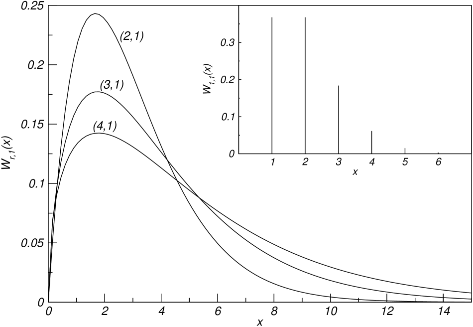
Figure 1: The weight functions $W_{r,1}(x)$, ($x=|z|^{2}$), in the resolution of unity for $r=2,3,4$ (continuous curves) and for $r=1$, a Dirac’s comb (in the inset), as a function of $x$.

the height of the vertical line at $x=k$ symbolizes the strength of the delta function $\delta(x-k)$, see Eq.(63). For further properties of $W_{1,1}(x)$ and more generally of $W_{r,r}(x)$ associated with Eq.(60), see [BPS04].

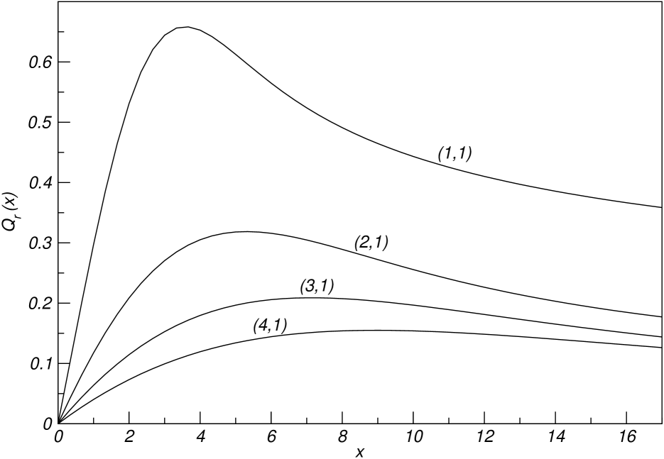
Figure 2: Mandel parameters $Q_{r}(x)$, for $r=1\ldots 4$, as a function of $x=|z|^{2}$, see Eq.(71).

Construction and properties

A comparison of Eqs.(56), (57) and (64) indicates that the normalized states defined through $\rho(n)=B_{r,1}(n+1)$ as

$$|z\rangle_{r}=\mathcal{N}_{r}^{-1/2}(|z|^{2})\sum_{n=0}^{\infty}\frac{z^{n}}{\sqrt{B_{r,1}(n+1)}}|n\rangle,$$ (68)

with normalization

$$\mathcal{N}_{r}(x)=\sum_{n=0}^{\infty}\frac{x^{n}}{B_{r,1}(n+1)}>0,$$ (69)

automatically satisfy the resolution of unity condition of Eq.(55), since for $W_{r,1}(x)=\pi\frac{\tilde{W}_{r,1}(x)}{\mathcal{N}_{r}(x)}$:

$$\int_{\mathbb{C}}d^{2}z\ |z\rangle_{r}\tilde{W}_{r,1}(|z|^{2}){{}_{r}\langle z|}=I=\sum_{n=0}^{\infty}|n\rangle\langle n|.$$ (70)

Note that Eq.(68) is equivalent to Eq.(53) with the definition $[n]_{r}=B_{r,1}(n+1)/B_{r,1}(n)$, $n=0,1,2,\ldots$.
Having satisfied the completeness condition with the functions $W_{r,1}(x)$, $r=1,2,\ldots$ we now proceed to examine the quantum-optical fluctuation properties of the states $|z\rangle_{r}$. From now on we consider the $|n\rangle$’s to be eigenfunctions of the boson number operator $N=a^{\dagger}a$, i.e. $N|n\rangle=n|n\rangle$. The Mandel parameter [KPS01]

$$Q_{r}(x)=x\left(\frac{{\mathcal{N}_{r}}^{\prime\prime}(x)}{{\mathcal{N}_{r}}^{\prime}(x)}-\frac{{\mathcal{N}_{r}}^{\prime}(x)}{\mathcal{N}_{r}(x)}\right),$$ (71)

allows one to distinguish between the sub-Poissonian (antibunching effect, $Q_{r}<0$) and super-Poissonian (bunching effect, $Q_{r}>0$) statistics of the beam. In Figure 2 we display $Q_{r}(x)$ for $r=1\ldots 4$. It can be seen that all the states $|z\rangle_{r}$ in question are super-Poissonian in nature, with the deviation from $Q_{r}=0$, which characterizes the conventional coherent states, diminishing for $r$ increasing.

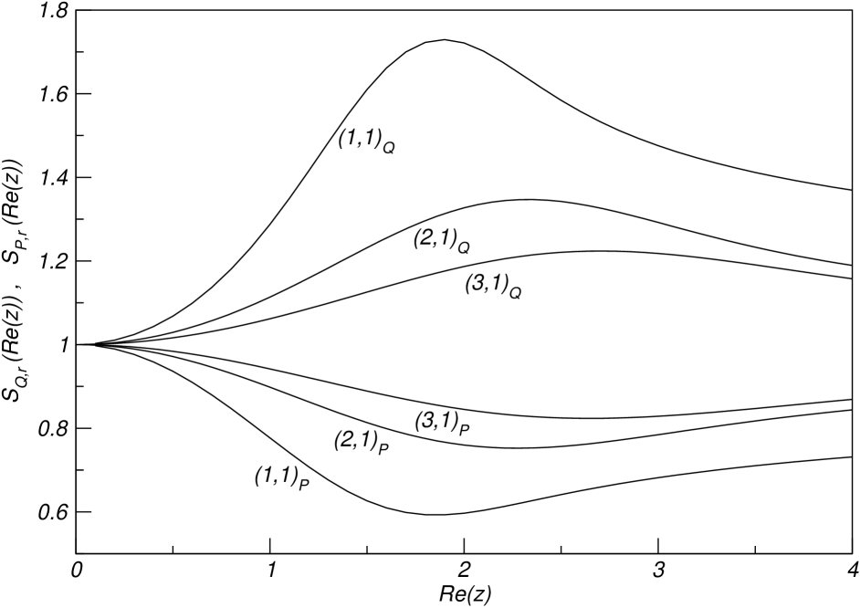
Figure 3: The squeezing parameters of Eqs.(72) and (73) for the coordinate $Q$ (three upper curves) and for the momentum $P$ (three lower curves) for different $r$, as a function of $Re(z)$, for $r=1,2,3$.

In Figure 3 we show the behavior of

$$S_{Q,r}(z)=\frac{{{}_{r}\langle z|(\Delta Q)^{2}|z\rangle_{r}}}{2},$$ (72)

and

$$S_{P,r}(z)=\frac{{{}_{r}\langle z|(\Delta P)^{2}|z\rangle_{r}}}{2},$$ (73)

which are the measures of squeezing in the coordinate and momentum quadratures respectively. In the display we have chosen the section along $Re(z)$. All the states $|z\rangle_{r}$ are squeezed in the momentum $P$ and dilated in the coordinate $Q$. The degree of squeezing and dilation diminishes with increasing $r$. By introducing the imaginary part in $z$ the curves of $S_{Q}(z)$ and $S_{P}(z)$ smoothly transform into one another, with the identification $S_{Q}(i\alpha)=S_{P}(\alpha)$ and $S_{P}(i\alpha)=S_{Q}(\alpha)$ for any positive $\alpha$.

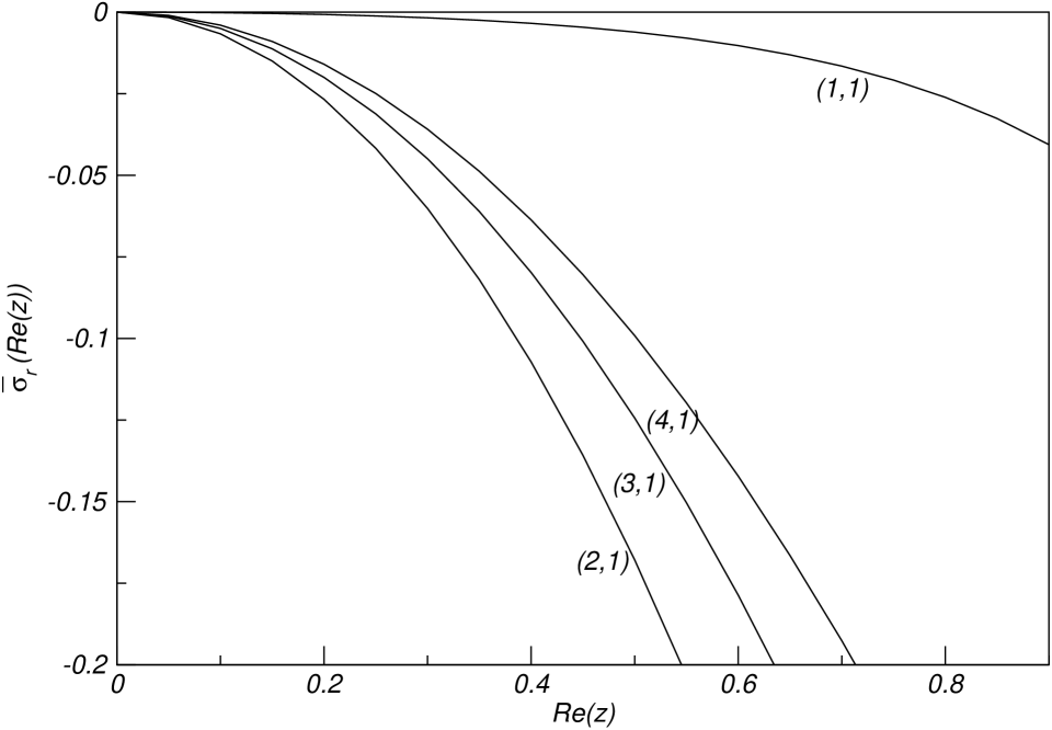
Figure 4: The signal-to-quantum noise ratio relative to its value in the standard coherent states $\bar{\sigma}_{r}$, see Eq.(74), as a function of $Re(z)$, for $r=1\ldots 4$.

In Figure 4 we show the signal-to-quantum noise ratio [Yue76] relative to $4[{{}_{c}\langle z|N|z\rangle_{c}}]=4|z|^{2}$, its value in conventional coherent states; i.e the quantity $\bar{\sigma}_{r}=\sigma_{r}-4[{{}_{c}\langle z|N|z\rangle_{c}}]$, where

$$\sigma_{r}=\frac{[{{}_{r}\langle z|Q|z\rangle_{r}}]^{2}}{(\Delta Q)^{2}},$$ (74)

with $(\Delta Q)^{2}={{}_{r}\langle z|Q^{2}|r\rangle_{r}}-({{}_{r}\langle z|Q|r\rangle_{r}})^{2}$. Again only the section $Re(z)$ is shown. We conclude from Figure 4 that the states $|z\rangle_{r}$ are more “noisy” than the standard coherent states with $\rho_{c}(n)=n!$ .
In Figure 5 we give the metric factors

$$\omega_{r}(x)=\left[x\frac{{\mathcal{N}_{r}}^{\prime}(x)}{\mathcal{N}_{r}(x)}\right]^{\prime},$$ (75)

which describe the geometrical properties of embedding the surface of coherent states in Hilbert space, or equivalently a measure of a distortion of the complex plane induced by the coherent states [KPS01]. Here, as far as $r$ is concerned, the state $|z\rangle_{1}$ appears to be most distant from the $|z\rangle_{c}$ coherent states for which $\omega_{c}=1$.

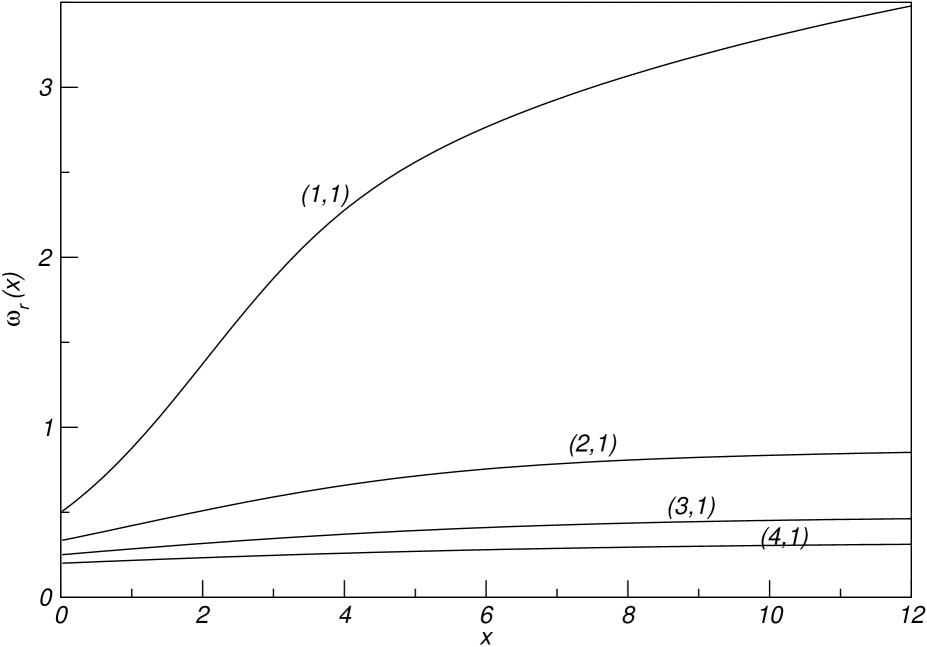
Figure 5: Metric factor $\omega_{r}(x)$, calculated with Eq.(75) as a function of $x=|z|^{2}$, for $r=1\ldots 4$.

Remarks

The use of sequences $B_{r,1}(n)$ to construct coherent states is not limited to the case exemplified by Eq.(68). In fact, any sequence of the form $B_{r,1}(n+p)$, $p=0,1,...$ will also define a set of coherent states, as then their respective weight functions will be $V_{r,1}^{(p)}(x)=x^{p-1}W_{r,1}(x)>0$. Will the physical properties of coherent states defined with $\rho_{p}(n)=B_{r,1}(n+p)$ depend sensitively on $p$ ? A case in point is that of $p=0$ for which qualitative differences from Figure 2 ($p=1$) appear. In Figure 7 we present the Mandel parameter for these states. Whereas for $r=1$ the state is still super-Poissonian, for $r=2,3,4$ one observes novel behavior, namely a crossover from sub- to super-Poissonian statistics for finite values of $x$. Also, as indicated in Figure 7, we note a cross-over between squeezing and dilating behavior for different $r$. These curious features merit further investigation.

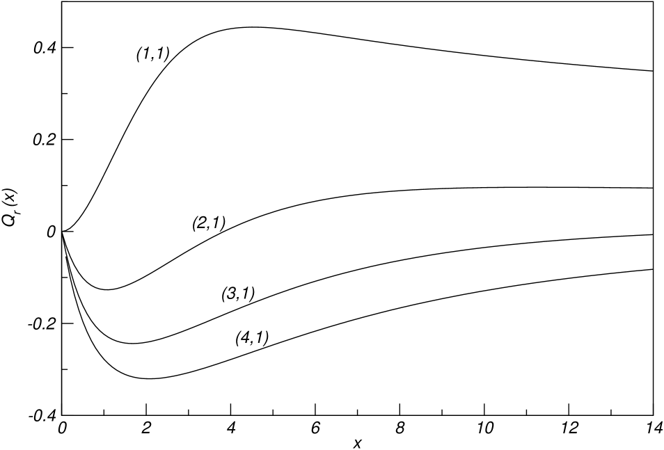
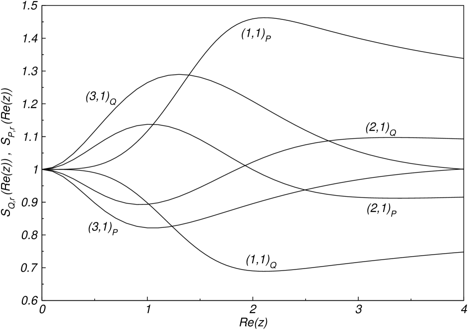
Figure 6: Mandel parameters $Q_{r}(x)$ for $r=1\ldots 4$, as a function of $x=|z|^{2}$, for states with $\rho(n)=B_{r,1}(n)$.

Figure 7: Squeezing parameters for the states with $\rho(n)=B_{r,1}(n)$ for $r=1,2,3$, as a function of $x=|z|^{2}$. The subscripts $P$ and $Q$ refer to momentum and coordinate variables respectively.

3 Substitution theorem

In Chapter 5 we have demonstrated how to find the normally ordered form of the exponential of the operator linear in the annihilation or creation operator. This representation is of fundamental meaning in the coherent state representation used in physics.
As a demonstration of possible other utility of such formulas we show the direct proof of the substitution theorem. More specifically we will demonstrate that for any function $F(x)$ the following equality holds

$$e^{\lambda\left(q(X)D+v(X)\right)}F(x)=G(\lambda,x)\cdot F(T(\lambda,x))$$ (76)

where functions $T(\lambda,x)$ and $G(\lambda,x)$ may be found from the following equations

$$\frac{\partial T(\lambda,x)}{\partial\lambda}=q(T(\lambda,x))\ , T(0,x)=x\ ,$$ (77)

$$\frac{\partial G(\lambda,x)}{\partial\lambda}=v(T(\lambda,x))\cdot G(\lambda,x)\ , G(0,x)=1\ .$$ (78)

First observe from Eq.(76) that the action of $e^{\lambda\left(q(X)D+v(X)\right)}$ on a function $F(x)$ amounts to:
a) change of argument $x\to T(\lambda,x)$ in $F(x)$ which is in fact a substitution;
b) multiplication by a prefactor $G(\lambda,x)$ which we call a prefunction.
We also see from Eq.(78) that $G(\lambda,x)=1$ for $v(x)=0$. Finally, note that $e^{\lambda\left(q(X)D+v(X)\right)}$ with $\lambda$ real generates an abelian, one-parameter group, implemented by Eq.(76); this gives the following group composition law for $T(\lambda,x)$ and $G(\lambda,x)$:

$$\begin{array}[]{ccl}T(\lambda+\theta,x)&=&T(\theta,T(\lambda,x)),\\ G(\lambda+\theta,x)&=&G(\lambda,x)\cdot G(\theta,T(\lambda,x)).\end{array}$$ (81)

Now we proceed to the proof of Eqs.(76)-(78). Using the multiplication $X$ and derivative $D$ representation we may rewrite Eq.(44) as

$$e^{\lambda\left(q(X)D+v(X)\right)}=\ :G(\lambda,X)\cdot e^{[T(\lambda,X)-X]D}:\$$ (82)

with accompanying differential Eqs.(41) and (42) for functions $T(\lambda,x)$ and $G(\lambda,x)$ which are exactly the same as Eqs.(77) and (78).
Now, recalling the Taylor formula $e^{\alpha D}F(x)=F(x+\alpha)$ we may generalize it to

$$:e^{\alpha(X)D}:\ F(x)=F(x+\alpha(x)).$$ (83)

It can be seen from the power series expansion of the exponential.
This allows to write

$$e^{\lambda\left(q(X)D+v(X)\right)}F(x) = :G(\lambda,X)\cdot e^{[T(\lambda,X)-X]D}:F(x)\$$

$$= G(\lambda,X)\ :e^{[T(\lambda,X)-X]D}:F(x)\$$

$$\stackrel{{\scriptstyle(\ref{gentaylor})}}{{=}} G(\lambda,X)\ F(x+[T(\lambda,x)-x])$$

$$= G(\lambda,x)\cdot F(T(\lambda,x)).$$

This completes the proof.
Here we list several examples illustrating Eqs.(76)-(78) for some choices of $q(x)$ and $v(x)$. Since Eqs.(77) and (78) are first order linear differential equations we shall simply write down their solutions without dwelling on details. First we treat the case of $v(x)=0$, which implies $g(\lambda,x)\equiv 1$:

• $$q(x)=x,\ \ \ \ \ \ \ \ \ T(\lambda,x)=xe^{\lambda}$$

  which gives $\exp\left(\lambda x\frac{d}{{d}x}\right)F(x)=F(xe^{\lambda})$, a well known illustration of the Euler dilation operator $\exp\left(\lambda x\frac{d}{{d}x}\right)$.

• $$q(x)=x^{r},\ \ r>1,\ \ \ \ \ \ \ \ \ T(\lambda,x)=\frac{\displaystyle x}{\displaystyle\left(1-\lambda\left(r-1\right)x^{r-1}\right)^{\frac{1}{r-1}}}$$

The above examples were considered in the literature [DOTV97][Lan00][BPS03b][BPS03c].
We shall go on to examples with $v(x)\neq 0$ leading to nontrivial prefunctions:

• $$q(x)=1\ \ \ \text{and}\ \ \ v(x)\ -\ \text{arbitrary},$$

  $$T(\lambda,x)=x+\lambda,$$

  $$g(\lambda,x)=e^{\int\limits_{0}^{\lambda}{\rm d}u\ v(x+u)}.$$

• $$q(x)=x,\ \ \ \text{and}\ \ \ v(x)=x^{2}$$

  $$T(\lambda,x)=xe^{\lambda},$$

  $$g(\lambda,x)=\exp{\left[\frac{x^{2}}{2}\left(e^{2\lambda}-1\right)\right]}.$$

• $$q(x)=x^{r}\ \ r>1\ \ \ \text{and}\ \ \ v(x)=x^{s}$$

  $$T(\lambda,x)=\frac{\displaystyle x}{\displaystyle\left(1-\lambda\left(r-1\right)x^{r-1}\right)^{\frac{1}{r-1}}}$$

  $$g(\lambda,x)=\exp{\left[\frac{\displaystyle x^{s-r+1}}{\displaystyle 1-r}\left(\frac{\displaystyle 1}{\displaystyle\left(1-\lambda\left(r-1\right)x^{r-1}\right)^{\frac{s-r+1}{r-1}}}-1\right)\right]}.$$

Closer inspection of the above examples (or at any other example which the reader may easily construct) indicates that from the analytical point of view the substitution theorem should be supplemented by some additional assumptions, like restrictions on $\lambda$. In general we can say that it can be valid only locally [DPS⁺04]. However, we note that a formulation in the language of formal power series does not require such detailed analysis and the resulting restrictions may be checked afterwords.
We finally note that the substitution theorem can be used to find the normally ordered form of an exponential operator linear in $a$ or $a^{\dagger}$ (as in Chapter 5). This idea has been exploited in [BHP⁺05].

Chapter 7 Conclusions

In this work we have considered the boson normal ordering problem for powers and exponentials of two wide classes of operators. The first one consists of boson strings and more generally homogenous polynomials, while the second one treats operators linear in one of the creation or annihilation operators. We have used the methods of advanced combinatorial analysis to obtain a thorough understanding and efficient use of the proposed formalism. In all cases we provided closed form expressions, generating functions, recurrences etc. The analysis was based on the Dobiński-type relations and the umbral calculus methods. In general, the combinatorial analysis is shown to be an effective and flexible tool in this kind of problem.
We also provided a wealth of examples and pointed out possible applications. The advantages may be neatly seen from the coherent state perspective (e.g. we may use it for construction of the phase space pictures of quantum mechanics). We may also obtain solutions of the moment problem, enabling us to construct new families of generalized coherent states. Moreover application to the operator calculus is noted and exemplified in the substitution theorem. We also observe that the normal ordering problems for deformed algebras may be handled within that setting.
These few remarks on the possible applications and extensions of the methods used in this work (others may be found in the supplied references) yield a potentially wide field of possible future research.
We would like to point out some other interesting features. We believe that similar combinatorial methods may be used to find the normally ordered forms of other classes of operators, such as the exponential of a general boson polynomial. Moreover, the extension to the multi-mode boson and fermion case should be susceptible to explicit analysis. This program would open a wide arena for immediate application to variety of physical models.
In conclusion, we would like to recall that the use of advanced combinatorics provides a wealth of interpretative tools for the problems under consideration. Combinatorial objects may be interpreted in terms of graphs, rook polynomials, partitions, correlations etc. We have not touched upon this aspect in this work but we consider it as a very promising one.

Chapter 8 Coherent states

Here we define and review some properties of coherent states [KS85][ZFR90].
We define coherent states $|z\rangle$ as the eigenstates of the annihilation operator

$$a|z\rangle=z|z\rangle,$$ (1)

where $z\in\mathbb{C}$ is a complex number. They can be written explicitly as

$$|z\rangle=e^{-\frac{1}{2}|z|^{2}}\ \sum_{n=0}^{\infty}\frac{z^{n}}{\sqrt{n!}}|n\rangle.$$ (2)

These states are normalized but not orthogonal. The coherent states overlapping factor is

$$\langle z|z^{\prime}\rangle=e^{z^{*}z^{\prime}-\frac{1}{2}|z^{{}^{\prime}}|^{2}-\frac{1}{2}|z|^{2}},$$ (3)

The set of coherent states $\left\{|z\rangle:\ z\in\mathbb{C}\right\}$ constitute an overcomplete basis in the Hilbert space $\cal{H}$. The following resolution of unity property holds

$$\frac{1}{\pi}\int_{\mathbb{C}}|z\rangle\langle z|\ d^{2}z=1.$$ (4)

Eq.(2) may be rewritten in the form (see Eqs.(8))

$$|z\rangle=e^{-\frac{|z|^{2}}{2}}e^{za^{\dagger}}|0\rangle,$$ (5)

or with the use of Eq.(27) as

$$|z\rangle=e^{za^{\dagger}-z^{*}a}|0\rangle.$$ (6)

The operator $D(z)=e^{za^{\dagger}-z^{*}a}$ is called a displacement operator and therefore coherent states are sometimes called displaced vacuum. This group property may be taken as the definition of the coherent states also for other (than Heisenberg-Weyl) groups, see [Per86].
Let us define two self-adjoint operators $Q$ and $P$ by

$$\begin{array}[]{rcl}Q&=&\frac{\displaystyle a^{\dagger}+a}{\displaystyle\sqrt{2}},\vspace{2mm}\\ P&=&i\ \frac{\displaystyle a^{\dagger}-a}{\displaystyle\sqrt{2}}.\end{array}$$ (9)

They satisfy the Heisenberg-Weyl commutation relation $[Q,P]=i$. These operators may be interpreted as the position and momentum operators for the quantum particle in the harmonic oscillator potential, in quantum optics they play the role of the field quadratures and are also used in the phase space formulation of Quantum Mechanics. It can be shown that the coherent states are the minimum uncertainty states for operators $Q$ and $P$, i.e.

$$\Delta_{|z\rangle}Q\cdot\Delta_{|z\rangle}P=\frac{1}{2},$$ (10)

where $\Delta_{\psi}A=\sqrt{\langle\psi|(A-\langle\psi|A|\psi\rangle)^{2}|\psi\rangle}$ is the uncertainty of the operator $A$. Moreover they are the only states if one additionally imposes the condition $\Delta_{|z\rangle}Q=\Delta_{|z\rangle}P$ (otherwise the family of squeezed states is obtained) which serves as another possible definition of coherent states.
Finally we mention that the resolution of unity of Eq.(4) together with the continuity of the mapping $z\to|z\rangle$ are sometimes taken as the minimum requirements for the coherent states. However, this definition is not unique and leads to other families of so called generalized coherent states [Kla63a][Kla63b][KS85] (see also Section 2).
We note that, due to their special features, coherent states are widely used in quantum optics [Gla63][KS68] as well as in other areas of physics [KS85].
In this text we especially exploit the property of Eq.(1). It is because for an operator $F(a,a^{\dagger})$ which is in the normal form, $F(a,a^{\dagger})\equiv{\cal N}\left[F(a,a^{\dagger})\right]\equiv\ :F(a,a^{\dagger}):$, its coherent state matrix elements may be readily written as

$$\langle z|F(a,a^{\dagger})|z^{\prime}\rangle=\langle z|z^{\prime}\rangle\ F(z^{\prime},z^{*}).$$ (11)

Also for the double dot operation it immediately yields

$$\langle z|:G(a,a^{\dagger}):|z^{\prime}\rangle=\langle z|z^{\prime}\rangle\ G(z^{\prime},z^{*}).$$ (12)

Unfortunately for the general operator none of these formulae hold. Nevertheless, there is a very useful property which is true; that is, if for an arbitrary operator $F(a,a^{{\dagger}})$ we have

$$\langle z|{F}(a,a^{{\dagger}})|z^{\prime}\rangle=\langle z|z^{\prime}\rangle\ G(z^{*},z^{\prime})$$ (13)

then the normally ordered form of ${F}(a,a^{{\dagger}})$ is given by

$${\cal N}\left[{F}(a,a^{{\dagger}})\right]=\ :G(a^{{\dagger}},a):\,.$$ (14)

For other properties of coherent states we refer to [KS85][ZFR90].

Chapter 9 Formal power series. Umbral calculus

Here we recall the basic definitions and theorems concerning the formal power series calculus. As an illustration some topics of the umbral calculus are reviewed. For a detailed discussion see [Niv69], [Com74], [Rio84], [Wil94], [GKP94], [FS05], [Rom84], [Rai65], [RR78], [Buc98].

Formal power series

Suppose we are given a series of numbers $(f_{n})_{n=0}^{\infty}$. We define a formal power series in indeterminate $x$ as

$$F(x)=\sum_{n=0}^{\infty}f_{n}\frac{x^{n}}{n!}.$$ (1)

The set of formal power series constitutes a ring when the following operations are imposed

• addition:

  $$F(x)+G(x)=\sum_{n=0}^{\infty}f_{n}\frac{x^{n}}{n!}+\sum_{n=0}^{\infty}g_{n}\frac{x^{n}}{n!}=\sum_{n=0}^{\infty}(f_{n}+g_{n})\frac{x^{n}}{n!}$$ (2)

• multiplication (Cauchy product rule):

  $$F(x)\cdot G(x)=\sum_{n=0}^{\infty}f_{n}\frac{x^{n}}{n!}\cdot\sum_{n=0}^{\infty}g_{n}\frac{x^{n}}{n!}=\sum_{n=0}^{\infty}\sum_{k=0}^{n}\binom{n}{k}f_{k}g_{n-k}\frac{x^{n}}{n!}$$ (3)

Both operations have an inverses. The inverse of the series $F(x)$ with respect to addition is the series with negative coefficients $-F(x)=\sum_{n=0}^{\infty}-f_{n}\frac{x^{n}}{n!}$. The (unique) multiplicative inverse on the other hand is well defined only when $f_{0}\neq 0$ and may be given recursively, see e.g. [Wil94].
One can also define the substitution of formal power series by

$$F(G(x))=\sum_{n=0}^{\infty}f_{n}\frac{G(x)^{n}}{n!}$$ (4)

when $g_{0}=0$ in the expansion $G(x)=\sum_{n=0}^{\infty}g_{n}\frac{x^{n}}{n!}$. Explicit expression for the coefficients is given by the Faà di Bruno formula [Com74][Ald01]. A series $F(x)$ may be shown to have a compositional inverse $F^{-1}(x)$ iff $f_{0}=0$ and $f_{1}\neq 0$.
Other definitions and properties can be further given. Here is the example of the derivative and integral of the formal power series (note that these operators act like shift operators on the sequence $(f_{n})_{n=0}^{\infty}$)

$$DF(x)=F^{\prime}(x)=\sum_{n=1}^{\infty}f_{n}\frac{x^{n-1}}{(n-1)!}=\sum_{n=0}^{\infty}f_{n+1}\frac{x^{n}}{n!}$$ (5)

$$\int F(x)\ dx=\sum_{n=0}^{\infty}f_{n}\frac{x^{n+1}}{(n+1)!}=\sum_{n=1}^{\infty}f_{n-1}\frac{x^{n}}{n!}$$ (6)

Observe that these definitions mirror the corresponding operations on analytic functions. Nevertheless the limiting operations are not needed in these definitions. The ring of formal power series can be also be given the structure of a complete metric space (see e.g. [FS05], [Rom84]).
We note that $(f_{n})_{n=0}^{\infty}$ may be also a sequence of polynomials, functions or anything else.
The use of power series is well suited in the context of generating functions. The series as in Eq.(1) is called the exponential generating function (because of the factor $1/n!$ in the expansion). Functions $G(x)=\sum_{n=0}^{\infty}g_{n}x^{n}$ are called ordinary generating functions. The use of generating functions is especially useful in solving recurrences and enumerating combinatorial objects, see eg. [Wil94][GKP94][FS05].
All these definitions and properties may be naturally extended to the multivariable case.
For a systematic description of the formal power series and applications see [Niv69], [Com74], [Rio84], [Wil94], [GKP94], [FS05], [Rom84].

Umbral calculus. Sheffer-type polynomials

Subject of the umbral calculus is the study of a Sheffer A-type zero polynomials, called here briefly Sheffer-type [She39], [Rai65]. Without going into details we recall some basic theorems and definitions [Rom84], [RR78], [Buc98].
Suppose we have a polynomial sequence $s_{n}(x)$, $n=0,1,2,...$ ($s_{n}(x)$ being the polynomial of degree $n$). It is called of a Sheffer-type if it possesses an exponential generating function of the form

$$G(\lambda,x)=\sum_{n=0}^{\infty}s_{n}(x)\frac{\lambda^{n}}{n!}=A(\lambda)e^{xB(\lambda)}.$$ (7)

for some (possibly formal) functions $A(\lambda)$ and $B(\lambda)$ such that $B(0)=0$, $B^{\prime}(0)\neq 0$ and $A(0)\neq 0$. When $B(\lambda)=1$ it is called Apple sequence for $A(\lambda)$. For $A(\lambda)=1$ it is known as associated sequence for $B(\lambda)$.
Yet another definition of the Sheffer-type sequences can be given through their lowering and rising operators, i.e. the polynomial sequence $s_{n}(x)$ is of Sheffer-type iff there exist some functions $f(x)$ and $g(x)$ (possibly formal) such that $f(0)=0$, $f^{{}^{\prime}}(0)\neq 0$ and $g(0)\neq 0$ which satisfy

$$f(D)s_{n}(x)=ns_{n-1}(x),$$ (8)

$$\left[X-\frac{g^{\prime}(D)}{g(D)}\right]\frac{1}{f^{\prime}(D)}s_{n}(x)=s_{n+1}(x).$$ (9)

These two definitions describe the Sheffer-type sequence uniquely and the correspondence is given by

$$A(x)=f^{-1}(x),$$ (10)

$$B(x)=\frac{1}{g(f^{-1}(x))}.$$ (11)

Many curious properties of the Sheffer-type polynomials can be worked out. We quote only one of them, called the Sheffer identity, to show the simplicity of formal manipulations. Using definition Eq.(7) we have

$$\sum_{n=0}^{\infty}s_{n}(x+y)\frac{\lambda^{n}}{n!} = A(\lambda)e^{(x+y)B(\lambda)}=A(\lambda)e^{xB(\lambda)}e^{yB(\lambda)}$$

$$= \sum_{n=0}^{\infty}s_{n}(x)\frac{\lambda^{n}}{n!}\cdot\sum_{n=0}^{\infty}p_{n}(y)\frac{\lambda^{n}}{n!}.$$

By the Cauchy product rule Eq.(3) we obtain the Sheffer identity:

$$s_{n}(x+y)=\sum_{k=0}^{n}\binom{n}{k}p_{k}(y)s_{n-k}(x)$$ (12)

where $p_{n}(x)$ is the associated sequence for $B(\lambda)$. Observe that for associated sequences ($A(\lambda)=1$) this property generalizes the binomial identity and therefore sometimes they are called of binomial type.
The Sheffer-type polynomials constitute a basis in the space of polynomials and through that property any formal power series can be developed in that basis also. On the other hand, formal power series can be treated as functionals on the space of polynomials. Investigation of this connection is also the subject of umbral calculus in which the Sheffer-type polynomials play a prominent role [Rom84].
We emphasize that all the functions and series here can be formal and then the operations are meant in the sense of the previous Section.
Thorough discussion of the umbral calculus, Sheffer-type polynomials and applications can be found in [Rom84][RR78][Buc98][Rai65].

List of Publications

Journal publications

• P. Błasiak, K.A. Penson and A.I. Solomon
  The general boson normal ordering problem
  Phys. Lett. A 309 198-205 (2003)
  arXiv:quant-ph/0402027

• P. Błasiak, K.A. Penson and A.I. Solomon
  Dobiński-type relations and the log-normal distribution
  J. Phys. A: Math. Gen. 36 L273-L278 (2003)
  arXiv:quant-ph/0303030

• P. Błasiak, K.A. Penson and A.I. Solomon
  The boson normal ordering problem and generalized Bell numbers
  Ann. Combinat. 7 127-139 (2003)
  arXiv:quant-ph/0212072

• P. Błasiak, A. Horzela and E. Kapuścik
  Alternative hamiltonians and Wigner quantization
  J. Opt. B: Quantum Semiclass. Opt. 5 S245-S260 (2003)

• P. Błasiak and A. Horzela
  Quantization of alternative Hamiltonians
  Czech. J. Phys. 53 985-991 (2003)

• K.A. Penson, P. Błasiak, G. Duchamp, A. Horzela
  and A.I. Solomon
  Hierarchical Dobiński-type relations via substitution and the moment problem
  J. Phys. A: Math. Gen. 37 3475-3487 (2004)
  arXiv:quant-ph/0312202

• P. Błasiak, K.A. Penson and A.I. Solomon
  Combinatorial coherent states via normal ordering of bosons
  Lett. Math. Phys. 67 13-23 (2004)
  arXiv:quant-ph/0311033

• P. Błasiak, A. Horzela, K. A. Penson, A.I. Solomon
  Deformed bosons: Combinatorics of the normal ordering
  Czech. J. Phys. 54 1179-1184 (2004)
  arXiv:quant-ph/0410226

• P. Błasiak, K.A. Penson, A.I. Solomon, A. Horzela
  and G. H. E. Duchamp
  Some useful combinatorial formulas for bosonic operators
  J. Math. Phys. 46 052110 (2005)
  arXiv:quant-ph/0405103

• P. Błasiak, A. Horzela, K.A. Penson, G.H.E. Duchamp
  and A.I. Solomon
  Boson Normal Ordering via Substitutions and Sheffer-type Polynomials
  Phys. Lett. A 338 108-116 (2005)
  arXiv:quant-ph/0501155

• M.A. Méndez, P. Błasiak and K.A. Penson
  Combinatorial approach to generalized Bell and Stirling numbers and boson normal ordering problem
  J. Math. Phys., in print (2005)
  arXiv:quant-ph/0505180

Conference proceedings

• A.I. Solomon, P. Błasiak, G. Duchamp, A. Horzela
  and K.A. Penson
  Combinatorial physics, normal order and model Feynman graphs
  Symmetries in Science XI
  B. Gruber, G. Marmo and N. Yoshinaga (eds.), p.527-536 (Kluwer Academic Publishers 2004)
  arXiv:quant-ph/0310174

• A.I. Solomon, G. Duchamp, P. Błasiak, A. Horzela
  and K.A. Penson
  Normal Order: Combinatorial Graphs
  Quantum Theory and Symmetries
  Proceedings of the 3rd International Symposium
  P.C. Argyres, T.J. Hodges, F. Mansouri, J.J. Scanio, P. Suranyi, L.C.R. Wijewardhana (eds.), p.398-406 (World Scientific Publishing 2004)
  arXiv:quant-ph/0402082

• G. Duchamp, K.A. Penson, A.I. Solomon, A. Horzela
  and P. Błasiak
  One-Parameter Groups and Combinatorial Physics
  Proceedings of the Third International Workshop on
  Contemporary Problems in Mathematical Physics
  (Cotonu, Bénin, November 1st-7th 2003)
  J. Govaerts, M.N. Hounkonnou and A.Z. Msezane (eds.)
  p. 436-449 (World Scientific Publishing, 2004)
  arXiv:quant-ph/0401126

• A.I. Solomon, P. Błasiak, G. Duchamp, A. Horzela
  and K.A. Penson
  Partition functions and graphs: A combinatorial approach
  Proceedings of the XI International Conference on Symmetry Methods in Physics (SYMPHYS-11) (Prague, Czech Republic, June 2004), in press (JINR Publishers, Dubna)
  arXiv:quant-ph/0409082

• A. Horzela, P. Błasiak, G.E.H. Duchamp, K.A. Penson
  and A.I. Solomon
  A product formula and combinatorial field theory
  Proceedings of the XI International Conference on Symmetry Methods in Physics (SYMPHYS-11) (Prague, Czech Republic, June 2004), in press (JINR Publishers, Dubna)
  arXiv:quant-ph/0409152

Preprints

• P. Błasiak, G. Dattoli, A. Horzela and K.A. Penson
  Representations of Monomiality Principle with Sheffer-type Polynomials and Boson Normal Ordering
  J. Phys. A: Math. Gen., submitted (2005)
  arXiv:quant-ph/0504009

• P. Błasiak, A. Horzela, K.A. Penson and A.I. Solomon
  Combinatorics of generalized Kerr models
  in preparation (2005)

References

• [Ald01] R. Aldrovandi. Special Matrices of Mathematical Physics. World Scientific, Singapore, 2001.
• [AM77] G. P. Agarawal and C. L. Mehta. Ordering of the exponential of a quadratic in boson operators. II. Multimode case. J. Math. Phys., 18:408–409, 1977.
• [Bar61] V. Bargmann. On a Hilbert space of analytic functions and an associated integral transform. Commun. Pure and Appl. Math., 14:187–214, 1961.
• [BDHP05] P. Blasiak, G. Dattoli, A. Horzela, and K.A. Penson. Representations of monomiality principle with Sheffer-type polynomials and boson normal ordering. 2005. arXiv:quant-ph/0504009.
• [Ben91] C. M. Bender. Solution of operator equations of motion. In J. Dittrich and P. Exner, editors, Rigorous Results in Quantum Dynamics, pages 99–112, Singapore, 1991. World Scientific.
• [BHP+05] P. Blasiak, A. Horzela, K.A. Penson, G.H.E. Duchamp, and A.I. Solomon. Boson normal ordering via substitutions and Sheffer-type polynomials. Phys. Lett. A, 338:108–116, 2005. arXiv:quant-ph/0501155.
• [BHPS05] P. Blasiak, A. Horzela, K.A. Penson, and A. I. Solomon. Combinatorics of generalized Kerr models. 2005.
• [BN05] C. Burdik and O. Navratil. Normal ordering for the deformed Heisenberg algebra involving the reflection operator. J. Phys. A : Math. Gen., 38:2305–2310, 2005.
• [BPS03a] P. Blasiak, K. A. Penson, and A. I. Solomon. Dobiński-type relations and the log-normal distribution. J. Phys. A: Math. Gen., 36:L273–L278, 2003. arXiv:quant-ph/0303030.
• [BPS03b] P. Blasiak, K.A. Penson, and A.I. Solomon. The boson normal ordering problem and generalized Bell numbers. Ann. Combinat., 7:127–139, 2003.
• [BPS03c] P. Blasiak, K.A. Penson, and A.I. Solomon. The general boson normal ordering problem. Phys. Lett. A, 309:198–205, 2003.
• [BPS04] P. Blasiak, K. A. Penson, and A. I. Solomon. Hierarchical Dobiński-type via substitution and the moment problem. J. Phys. A: Math. Gen., 37:3475–3487, 2004. arXiv:quant-ph/0312202.
• [BPS+05] P. Blasiak, K. A. Penson, A. I. Solomon, A. Horzela, and G. H. E. Duchamp. Some useful combinatorial formulas for bosonic operators. J. Math. Phys., 46:052110, 2005. arXiv:quant-ph/0405103.
• [Buc98] A. Di Bucchianico. Introduction to umbral calculus. http://www.win.tue.nl/~sandro/, 1998.
• [Ces00] C. Cesarano. Monomiality principle and Legendre polynomials. In H. M. Srivastava G. Dattoli and C. Cesarano, editors, Advanced Special Functions and Integration Methods, page 147. Rome: Aracne Rditrice, 2000.
• [CG69] K. E. Cahill and R.J. Glauber. Ordered expansions in boson amplitude operators. Phys.Rev., 177:1857–1881, 1969.
• [CGH+96] R. M. Corless, G. H. Gonnet, D. E. G. Hare, D. J. Jeffrey, and D. E. Knuth. On the Lambert W function. Adv. Comp. Math., 5:329–359, 1996.
• [Che03] Y. Ben Cheikh. Some results on quasi-monomiality. Appl. Math. Comput., 141:63–76, 2003.
• [Com74] L. Comtet. Advanced Combinatorics. Reidel, Dordrecht, 1974.
• [Das96] A. DasGupta. Disentanglement formulas: An alternative derivation and some applications to squeezed coherent states. Am. J. Phys., 64:1422–1427, 1996.
• [Dat99] G. Dattoli. Hermite-Bessel and Laguerre-Bessel functions: a by-product of the monomiality principle. In G. Dattoli D. Cocolicchio and H. M. Srivastava, editors, Advanced Special Functions and Applications, page 83. Rome: Aracne Rditrice, 1999.
• [DOTV97] G. Dattoli, P.L. Ottaviani, A. Torre, and L. Vasquez. Evolution operator equations: Integration with algebraic and finite-difference methods. Applications to physical problems in classical and quantum mechanics and quantum field theory. Riv. Nuovo Cim., 20:1–133, 1997.
• [DPS+04] G. Duchamp, K. A. Penson, A. I. Solomon, A. Horzela, and P. Blasiak. One-parameter groups and combinatorial physics. In M. N. Hounkonnou J. Govaerts and A. J. Msezane, editors, Contemporary Problems in Mathematical Physics, pages 436–449, Singapore, 2004. World Scientific. arXiv:quant-ph/0401126.
• [DSC01] G. Dattoli, H. M. Srivastava, and C. Cesarano. The Laguerre and Legendre polynomials from operational point of view. Appl. Math. Comput., 124:117, 2001.
• [FS05] P. Flajolet and R. Sedgewick. Analytic Combinatorics. http://algo.inria.fr/flajolet/Publications/books.html, 2005.
• [GDM97] A. Torre G. Dattoli and G. Mazzacurati. Quasimonomials and isospectral problems. Nuov. Cim. B, 112:133–138, 1997.
• [GKP94] R. L. Graham, D. E. Knuth, and O. Patashnik. Concrete Mathematics. Addison-Wesley, Massachusetts, 1994.
• [Gla63] R. J. Glauber. The quantum theory of optical coherence. Phys. Rev., 130:2529–2539, 1963.
• [Gro78] E. Grosswald. Bessel Polynomials. Springer, Berlin, 1978.
• [JPS01] J.M.Sixdeniers, K.A. Penson, and A.I. Solomon. Extended Bell and Stirling numbers from hypergeometric exponentiation. J. Int. Seqs., Article 01.1.04:1–11, 2001. http://www.research.att.com/~njas/sequences/JIS/.
• [Kat74] J. Katriel. Combinatorial aspects of boson algebra. Lett. Nuovo Cimento, 10:565–567, 1974.
• [Kat83] J. Katriel. Normal ordering formulae for some boson operators. J. Phys. A : Math. Gen., 16:4171–4173, 1983.
• [Kat00] J. Katriel. Bell numbers and coherent states. Phys. Lett. A, 237:159–161, 2000.
• [Kat02] J. Katriel. Coherent states and combinatorics. J. Opt. B: Quantum Semiclass. Opt., 4:S200–S203, 2002.
• [KD95] J. Katriel and G. Duchamp. Ordering relations for $q$-boson operators, continued fraction techniques and the $q$-BCH enigma. J. Phys. A : Math. Gen., 28:7209–7225, 1995.
• [KK92] J. Katriel and M. Kibler. Normal ordering for deformed boson operators and operator-valued deformed Stirling numbers. J. Phys. A: Math. Gen., 25:2683–2691, 1992.
• [Kla63a] J. R. Klauder. Continuous-representation theory. I. Postulates for continuous-representation theory. J. Math. Phys, 4:1055–1058, 1963.
• [Kla63b] J. R. Klauder. Continuous-representation theory. II. Generalized relation between quantum and classical dynamics. J. Math. Phys, 4:1058–1073, 1963.
• [KPS01] J. R. Klauder, K.A. Penson, and J.M. Sixdeniers. Constructing coherent states through solutions of Stieltjes and Hausdorff moment problems. Phys. Rev. A, 64:013817–013835, 2001.
• [KS68] J. R. Klauder and E. C. G. Sudarshan. Fundamentals of Quantum Optics. Benjamin, New York, 1968.
• [KS85] J. R. Klauder and B-S. Skagerstam. Coherent States. Application in Physics and Mathematical Physics. World Scientific, Singapore, 1985.
• [KVD01] Z. Kis, W. Vogel, and L. Davidovich. Nonlinear coherent states of trapped-atom motion. Phys. Rev. A, 64:033401–033411, 2001.
• [Lan00] W. Lang. On generalizations of the Stirling number triangles. J. Int. Seqs., Article 00.2.4:1–19, 2000. http://www.research.att.com/ njas/sequences/JIS/.
• [Lou64] W. H. Louisell. Radiation and Noise in Quantum Electronics. McGrow-Hill Co., New York, 1964.
• [MBP05] M.A. Méndez, P. Blasiak, and K. A. Penson. Combinatorial approach to generalized Bell and Stirling numbers and boson normal ordering problem. J. Math. Phys., 2005. arXiv:quant-ph/0505180.
• [Meh77] C. L. Mehta. Ordering of the exponential of a quadratic in boson operators. I. Single mode case. J. Math. Phys., 18:404–407, 1977.
• [Mik83] V. V. Mikhailov. Ordering of some boson operator functions. J. Phys. A : Math. Gen., 16:3817–3827, 1983.
• [Mik85] V. V. Mikhailov. Normal ordering and generalized Stirling numbers. J. Phys. A : Math. Gen., 18:231–235, 1985.
• [MM98] V. I. Manko and V.I. Vilela Mendes. On the nonlinearity interpretation of $q$- and $f$-deformations and some applicationss. J. Phys. A, 31:6037–6044, 1998.
• [MMSZ97] V. I. Manko, G. Marmo, E.C.G. Sudarshan, and F. Zaccaria. f-Oscilators and nonlinear coherent states. Phys.Scr., 55:528–541, 1997.
• [MSI93] A. Mufti, H. A. Schmitt, and M. Sargent III. Finite-dimensional matrix representations as calculational tools in quantum optics. Am. J. Phys., 6!:729–733, 1993.
• [MV96] V.I. Vilela Mendes and W. Vogel. Nonlinear coherent states. Phys. Rev. A, 54:4560–4563, 1996.
• [MW95] L. Mandel and R. Wolf. Optical Coherence and Quantum Optics. University Press, Cambridge, 1995.
• [Nav73] A.M. Navon. Combinatorics and fermion algebra. Nuovo Cimento, 16B:324–330, 1973.
• [Niv69] I. Niven. Formal power series. Am. Math. Monthly, 76:871–889, 1969.
• [Per86] A.M. Perelomov. Generalized Coherent States and Their Application. Springer-Verlag, Berlin, 1986.
• [Pit99] J. Pittman. A lattice path model for the Bessel polynomials. Technical Report 551, U.C. Berkeley, USA, 1999.
• [PS99] K. A. Penson and A. I. Solomon. Mittag-Leffler coherent states. J. Phys. A: Math. Gen., 32:7543–7563, 1999.
• [PS01] K. A. Penson and A. I. Solomon. Coherent states from combinatorial sequences. In 2nd International Symposium on Quantum Theory and Symmetries, pages 527–530, Singapore, 2001. World Scientific. arXiv:quant-ph/0111151.
• [Rai65] E.D. Rainville. Special Functions. The Macmillan Company, New York, 1965.
• [Rio84] J. Riordan. An Introduction to Combinatorial Analysis. Wiley, New York, 1984.
• [Rom84] S. Roman. The Umbral Calculus. Academic Press, Orlando, 1984.
• [RR78] S. Roman and G.-C. Rota. The umbral calculus. Adv. Math., 27:95–188, 1978.
• [Sch03] M. Schork. On the combinatorics of normal ordering bosonic operators and deformations of it. J. Phys. A: Math. Gen., 36:4651–4665, 2003.
• [SDB+04] A.I. Solomon, G.H.E. Duchamp, P. Blasiak, A. Horzela, and K.A. Penson. Normal order: Combinatorial graphs. In 3rd International Symposium on Quantum Theory and Symmetries, pages 527–536, Singapore, 2004. World Scientific. arXiv:quant-ph/0402082.
• [Seg63] I. Segal. Mathematical Problems of Relativistic Physics. Providence, Rhode Island, 1963.
• [She39] I.M. Sheffer. Some properties of polynomial sets of type zero. Duke Math. Journal, 5:590–622, 1939.
• [Six01] J. M. Sixdeniers. Constructions de nouveaux états cohérentes à l’aide de solutions des problèmes des moments. PhD thesis, Université Paris 6, 2001.
• [Slo05] N.J.A. Sloane. Encyclopedia of integer sequences. http://www.research.att.com/~njas/sequences, 2005.
• [Sol94] A.I. Solomon. A characteristic functional for deformed photon phenomenology. Phys. Lett. A, 196:29–34, 1994.
• [SP00] J. M. Sixdeniers and K. A. Penson. On the completeness of coherent states generated by binomial distribution. J. Phys. A: Math. Gen., 33:2907–2916, 2000.
• [SPK01] J. M. Sixdeniers, K. A. Penson, and J. R. Klauder. Tricomi coherent states. Int. J. Mod. Phys. B, 15:4231–4243, 2001.
• [ST79] D. Shalitin and Y. Tikochinsky. Transformation between the normal and antinormal expansions of boson operators. J. Math. Phys., 20:1676–1678, 1979.
• [Sta99] R.P. Stanley. Enumerative Combinatorics. University Press, Cambridge, 1999.
• [TS95] A. Turbiner and Y. Smirnov. Hidden SL2-algebra of finite difference equations. Mod. Phys. Lett. A, 10:1795–1801, 1995.
• [Var04] A. Varvak. Rook numbers and the normal ordering problem. In Formal Power Series and Algebraic Combinatorics, pages 259–268, University of British Columbia (Vancouver B.C., Canada), 2004. arXiv:math.CO/0402376.
• [Wil67] R.M. Wilcox. Exponential operators and parameter differentiation in quantum physics. J. Math. Phys., 8:962–982, 1967.
• [Wil94] H.S. Wilf. Generatingfunctionology. Academic Press, New York, 1994.
• [Wit75] W. Witschel. Ordered operator expansions by comparison. J. Phys. A : Math. Gen., 8:143–155, 1975.
• [Wit05] W. Witschel. Ordering of boson operator functions by the Hausdorff similarity transform. Phys. Lett. A, 334:140–143, 2005.
• [Yue76] H. P. Yuen. Two-photon coherent states of the radiational field. Phys. Rev. A, 13:2226–2243, 1976.
• [ZFR90] W. M. Zhang, D.H. Feng, and R.Gilmore. Coherent states: Theory and some applications. Rev. Mod. Phys., 62:867–927, 1990.