Hilbert-Schmidt Separability Probabilities and Noninformativity of Priors

Abstract

The Horodecki family employed the Jaynes maximum-entropy principle, fitting the mean ($b_{1}$) of the Bell-CHSH observable ($B$). This model was extended by Rajagopal by incorporating the dispersion ($\sigma_{1}^{2}$) of the observable, and by Canosa and Rossignoli, by generalizing the observable ($B_{\alpha}$). We further extend the Horodecki one-parameter model in both these manners, obtaining a three-parameter ($b_{1},\sigma_{1}^{2},\alpha$) two-qubit model, for which we find a highly interesting/intricate continuum $(-\infty<\alpha<\infty)$ of Hilbert-Schmidt (HS) separability probabilities — in which, the golden ratio is featured. Our model can be contrasted with the three-parameter ($b_{q},\sigma_{q}^{2},q$) one of Abe and Rajagopal, which employs a $q$(Tsallis)-parameter rather than $\alpha$, and has simply $q$-invariant HS separability probabilities of $\frac{1}{2}$. Our results emerge in a study initially focused on embedding certain information metrics over the two-level quantum systems into a $q$-framework. We find evidence that Srednicki’s recently-stated biasedness criterion for noninformative priors yields rankings of priors fully consistent with an information-theoretic test of Clarke, previously applied to quantum systems by Slater.

I Introduction

Both Rajagopal Rajagopal (1999), as well as Canosa and Rossignoli Canosa and Rossignoli (2005) have extended a well-known maximum-entropy model of the Horodecki family Horodecki et al. (1999) to two-parameter models, but in different fashions. Rajagopal incorporated the dispersion ($\sigma_{1}^{2}$) of the Bell-CHSH observable ($B$) Clauser et al. (1969), the mean ($b_{1}$) of which is already fitted in the Horodecki model, while Canosa and Rossignoli fitted the mean of generalized Bell-CHSH observables ($B_{\alpha}$). We combine their two approaches into a three-parameter ($b_{1},\sigma_{1}^{2},\alpha$) model, for which we uncover a very interesting continuum ($-\infty<\alpha<\infty$) of exact Hilbert-Schmidt separability probabilities (sec. VII.2.2, Fig. 11, (37)) — in which, among other features, the golden ratio Livio (2002); Markowsky (2004) appears.

Our model can be interestingly contrasted with a three-parameter ($b_{q},\sigma_{q}^{2},q$) one also of Abe and Rajagopal Abe and Rajagopal (1999) (sec. VII.2), which incorporates the $q$-parameter (nonextensitity/Tsallis index/escort parameter), rather than the $\alpha$-parameter of $B_{\alpha}$ (34). The continuum (over $q$) of separability probabilities (independently of the metric employed) is simply a constant (equal to $\frac{1}{2}$ in the Hilbert-Schmidt case, and to the “silver mean”, $\sqrt{2}-1$, for the Bures and other monotone metrics). We examine a two-parameter ($b_{1},\alpha$) Canosa-Rossignoli-type model also exhibiting an interesting (non-flat) continuum (sec. VII.2.3, Fig. 12, (38)). Additionally, we obtain exact (Hilbert-Schmidt and Bures) separability probabilities for the three-parameter Tsallis-Lloyd-Baranger model Tsallis et al. (2001) (sec. VII.3)

Our results emerge in a study initially focused on embedding certain information metrics over the two-level quantum systems into a $q$-framework. We find evidence (sec. V, Fig. 1) that Srednicki’s recently-stated biasedness criterion for noninformative priors Srednicki (2005) yields rankings of priors fully consistent with an information-theoretic test of Clarke Clarke (1996), previously applied to quantum systems by Slater Slater (1998).

II Noninformativity of Priors

Some fifteen years ago, Wootters asserted that “there does not seem to be any natural measure on the set of all mixed states” (Wootters, 1990, p. 1375). He did, however, consider random density matrices with all eigenvalues fixed. He remarked that once “the eigenvalues are fixed, then all the density matrices in the ensemble are related to each other by the unitary group, so it is natural to use the unique unitarily invariant measure to define the ensemble” (Wootters, 1990, p. 1375) (cf. Hall (1998)).

Arguing somewhat similarly, Srednicki recently proposed that in choosing a prior distribution over density matrices, “we can use the principle of indifference, applied to the unitary symmetry of Hilbert space, to reduce the problem to one of choosing a probability distribution for the eigenvalues of $\rho$. There is, however, no compelling rationale for any particular choice; in particular, we must decide how biased we are towards pure states” (Srednicki, 2005, p. 6).

To be specific, we find, in an analysis involving four prior probabilities ($p$’s), that the information-theoretic-based comparative noninformativity test devised by Clarke yields a ranking

$$p_{F_{q=1}}>p_{B}>p_{B_{q=1}trunc}>p_{F}$$ (1)

fully consistent (Fig. 1) with Srednicki’s recently-stated criterion for priors of “biasedness to pure states”. Two of the priors are formed by extending certain metrics of quantum-theoretic interest from three- to four-dimensions — by incorporating the $q$-parameter. The three-dimensional metrics are the Bures (minimal monotone) metric over the two-level quantum systems and the Fisher information metric over the corresponding family of Husimi distributions. The priors $p_{B}$ and $p_{F}$ are the (independent-of-$q$) normalized volume elements of these metrics, and $p_{F_{q=1}}$ is the normalized volume element of the $q$-extended Fisher information metric, with $q$ set to 1. While originally intended to similarly be the $q$-extension of the Bures metric, with $q$ then set to 1, the prior $p_{B_{q=1}trunc}$, actually entails the truncation of the only off-diagonal entry of the extended Bures metric tensor. Without this truncation, the $q$-extended Bures volume element is null, as is also the case in three higher-dimensional quantum scenarios we examine (including the Abe-Rajagopal two-qubit states (sec. VII.2), for which we further find $q$-invariant Bures separability probabilities equal to $\sqrt{2}-1$ [the “silver mean”] and Hilbert-Schmidt ones equal to $\frac{1}{2}$ (sec. VII.2.1), and the Tsallis-Lloyd-Baranger two-qubit states (sec. VII.3)).

III Bures Metric

The Bures (minimal monotone) metric — the volume element of which we normalize to obtain one ($p_{B}$) of the four prior probability distributions of principal interest here — yields the statistical distance between neighboring mixed quantum states ($\rho$) Braunstein and Caves (1994); Uhlmann (1976). It provides an embedding of the Fubini-Study metric (Petz and Sudár, 1996, sec. IV), which gives the statistical distance between neighboring pure quantum states ($|\psi\rangle$) (cf. Majtey et al. ). Hübner gave an explicit formula for the Bures distance (Hübner, 1992, p. 240) (cf. Luo and Zhang (2004)),

$$d_{B}(\rho_{1},\rho_{2})^{2}=2-2\mbox{tr}(\rho_{1}^{1/2}\rho_{2}\rho_{1}^{1/2})^{1/2}.$$ (2)

Further, he expressed it in infinitesimal form as (Hübner, 1992, eq. (10))

$$d_{B}(\rho,\rho+d\rho)^{2}=\Sigma_{ij}\frac{1}{2}\frac{|<i|d\rho|j>|^{2}}{\lambda_{i}+\lambda_{j}},$$ (3)

where the $\lambda_{i}$’s are the eigenvalues and the $|i\rangle$’s, the eigenvectors of $\rho$.

Figure 1: Four univariate marginal prior probability distributions in the near-to-pure-state region $r\in[1-\epsilon,1]$, where $r$ is the radial coordinate in the Bloch sphere representation of two-level quantum systems, and $r=1$ corresponds to a pure state. The order of dominance fully complies with that (1) obtained by the information-theoretic-based comparative noninformativity test

III.1 Three-Dimensional Case

In Slater (1996a), using the familiar Bloch sphere (unit ball in Euclidean 3-space) representation of the two-level quantum systems ($2\times 2$ density matrices),

$$\rho=\frac{1}{2}\left(\begin{array}[]{ccc}1+z&x-iy\\ x+iy&1-z\\ \end{array}\right),\hskip 36.135ptr^{2}=x^{2}+y^{2}+z^{2}\leq 1,$$ (4)

it was found (cf. (Hall, 1998, p. 128)), here converting from cartesian to spherical coordinates,

$$x=r\cos{\theta_{1}},\hskip 21.68121pty=r\sin{\theta_{1}}\cos{\theta_{2}},\hskip 21.68121ptz=r\sin{\theta_{1}}\sin{\theta_{2}},$$ (5)

that

$$d_{B}(\rho,\rho+d\rho)^{2}=\frac{1}{4}\Big{(}\frac{1}{(1-r^{2})}dr^{2}+dn^{2}\Big{)}.$$ (6)

The term $dr^{2}$ corresponds to the radial component of the metric and $dn^{2}$, the tangential component ($dn^{2}=r^{2}d\theta_{1}^{2}+r^{2}\sin^{2}{\theta_{2}}$). In the setting of the quantum monotone metrics — the Bures metric serving as the minimal monotone one — it is appropriate to express the tangential component of the Bures metric (6) in the form (Petz and Sudár, 1996, eq. (3.17)),

$$\Big{(}(1+r)f_{B}(\frac{1-r}{1+r})\Big{)}^{-1},$$ (7)

where $f_{B}(t)=\frac{1+t}{2}$ is an operator monotone function Lesniewski and Ruskai (1999).

The volume element of the Bures metric (7) is $\frac{r^{2}\sin{\theta_{1}}}{8(1-r^{2})}$, which can be normalized to a prior probability distribution over the Bloch sphere,

$$p_{B}=\frac{r^{2}\sin{\theta_{1}}}{\pi^{2}(1-r^{2})}.$$ (8)

III.2 Four-Dimensional Case

Now, we can construct a four-dimensional family of (properly normalized/unit trace) $2\times 2$ escort density matrices (cf. Naudts ),

$$\rho_{\{q\}}=\Big{(}(1-r)^{q}+(1+r)^{q}\Big{)}^{-1}\left(\begin{array}[]{ccc}1+z&x-iy\\ x+iy&1-z\\ \end{array}\right)^{q},$$ (9)

for which $q=1$ recovers the standard Bloch sphere representation (4). Applying Hübner’s formula (3), we have found that the extended Bures metric (now incorporating the $q$-parameter) has the form

$$d_{Bures_{q}}(\rho,\rho+d\rho)^{2}=\frac{1}{4(1+W^{q})^{2}}\Big{(}W^{q}\log^{2}{W}dq^{2}+\frac{4qW^{q}\log{W}}{r^{2}-1}dqdr+$$ (10)

$$+4\frac{q^{2}W^{q}}{(r^{2}-1)^{2}}dr^{2}+\frac{(-1+W^{q})^{2}}{r^{2}}dn^{2}\Big{)},$$

where $W=\frac{1-r}{1+r}$, that is, the ratio of the two eigenvalues of $\rho$.

The tangential component of the metric (10) can be expressed as $((1+r)f_{Bures_{q}}(W))^{-1}$, where

$$f_{Bures_{q}}(t)=\frac{2(1+t)(1+t^{q})^{2}}{(-1+t^{q})^{2}}.$$ (11)

This bivariate function appears (Fig. 2) to be monotonically-increasing for any fixed $q$ (cf. Petz and Sudár (1996)).

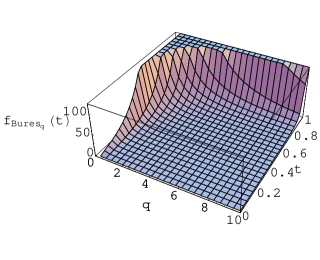
Figure 2: The function $f_{Bures_{q}}(t)$ that yields the tangential component (11) of the extended (four-dimensional) Bures metric (10)

Now, in the earlier stage of our analyses, due to a programming oversight, we were under the impression that the off-diagonal $dqdr$ term of (10) was simply zero. If we do employ the fully correct form, with this $dqdr$ term included, we find that the volume element is null. This, of course, could not yield a meaningful prior probability distribution. However, having proceeded under the impression that the $dqdr$ term was null, we obtained a number of results that appear to be of interest and of some relevance. Therefore, for much of this study, we will treat the $dqdr$ term as null, and thus deal with a truncated $q$-extended Bures metric.

In the context of the harmonic oscillators states, Pennini and Plastino have argued that, in addition to the physical lower bound (ignorance-amount) of $q\geq 0$ that in a quantal regime, $q$ can be no less than 1 Pennini and Plastino (2004) — due to the Lieb bound on the Wehrl entropy Lieb (1978). However, for the two-level quantum systems to the study of which we restrict ourselves here, the lower bound on the Wehrl entropy is $\frac{1}{2}$ (Schupp, 1999, eq. (12)). We, thus, consider $q\in[\frac{1}{2},\infty]$ to be the range of possible values of the escort parameter $q$. In practice, though, we will, for numerical and graphical purposes and normalization of the (divergent over $q\in[1/2,\infty]$) truncated extended Bures volume element (Sec. VI), consider that $q\in[\frac{1}{2},500]$.

In Fig. 3 we show the two-dimensional marginal volume element of (10) (after omission of the $dqdr$ term) — integrating out the spherical angles, $\theta_{1},\theta_{2}$, and leaving the radial coordinate $r$ and the escort parameter $q$.

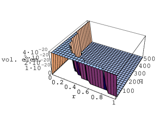
Figure 3: Two-dimensional marginal of the truncated four-dimensional extended Bures volume element (10)

In Fig. 4, further integrating out $r$, we show the corresponding one-dimensional marginal volume element of (10) (after omission of the $dqdr$ term) over $q$.

Figure 4: One-dimensional marginal (12) over $q$ of the four-dimensional truncated extended Bures volume element (10)

This (Fig. 4) has the exact expression

$$\frac{\pi(1+\log{4})}{24q}.$$ (12)

This prior, thus, conforms to Jeffreys’ rule — as opposed to the Bayes-Laplace rule, which would give a constant prior Slater (2000a).

In Fig. 5, we integrate out $q\in[\frac{1}{2},500]$, leaving a (deep bowl-shaped) one-dimensional marginal over $r\in[0,1]$. (The corresponding marginal in the unextended Bures case is $\frac{\pi r^{2}}{2(1-r^{2})}$, so it is simply increasing with $r$, in that case.) The associated indefinite integral over $q$ is

$$\frac{\pi\,\left(q\,W^{q}\,\left(3+W^{2\,q}\right)\,\log(W)-\left(1+W^{q}\right)\,\left(2\,W^{q}+{\left(1+W^{q}\right)}^{2}\,\log(1+W^{q})\right)\right)}{6\,\left(-1+r^{2}\right)\,{\left(1+W^{q}\right)}^{3}\,\log(W)}.$$ (13)

(So, we obtain the function plotted in Fig. 5 by substituting $q=500$ and $q=\frac{1}{2}$ into (13) and taking the difference.)

Figure 5: One-dimensional marginal (obtained from (13)) over $r$ of the four-dimensional extended Bures volume element (10) after omission of the off-diagonal $dqdr$ term

For $q=1$, the extended Bures metric (10) reduces to

$$ds_{Bures_{q=1}}(\rho,\rho+d\rho)^{2}=\frac{1}{16}(1-r^{2})\log^{2}{W}dq^{2}-\frac{1}{4}\log{W}dqdr+ds_{B}(\rho,\rho+d\rho)^{2}.$$ (14)

Normalizing the volume element of this metric — but first nullifying the off-diagonal $dqdr$ term — to a (non-null) prior probability distribution over the Bloch sphere, we obtain (cf. (8)),

$$p_{B_{q=1}trunc}=\frac{3}{4}\frac{r^{2}\sin{\theta_{1}}\log{\frac{1}{W}}}{\pi(1+\log{4})},$$ (15)

one of the four priors that we rank (Fig. 1 and (1)) both by the comparative noninformativity test and Srednicki’s biasedness criterion.

III.3 Comparative Noninformativities in the Bures Setting

The relative entropy (Kullback-Leibler distance/information gain Borland et al. (1998); Vedral (2002)) of $p_{B}$ with respect to $p_{B_{q=1}trunc}$ [which we denote $S_{KL}(p_{B},p_{B_{q=1}trunc})$] — that is, the expected value with respect to $p_{B}$ of $\log{\frac{p_{B}}{p_{B_{q=1}trunc}}}$ — is 0.101846 “nats” of information. Now, reversing arguments, $S_{KL}(p_{B_{q=1}trunc},p_{B})=0.0661775$. (We use the natural logarithm, and not 2 as a base, with one nat equalling 0.531 bits.) Let us convert — using Bayes’ rule — these two (prior) probability distributions to posterior probability distributions ($post_{B}$ and $post_{Bures_{q=1}}$), by assuming three pairs of spin measurements, one each in the x-, y- and z-direction, each pair yielding one “up” and one “down”. This gives us the likelihood function (cf. (Srednicki, 2005, eq. (9)) (Bagan et al., 2005, eq. (4.2))),

$$L(x,y,z)=\frac{(1-x^{2})(1-y^{2})(1-z^{2})}{64}$$ (16)

(which we convert to the spherical coordinates (5) in which we perform our Mathematica computations).

Then, we have $S_{KL}(post_{B}||p_{B_{q=1}trunc})=0.169782$ and $S_{KL}(post_{Bures_{q=1}}||p_{B})=0.197657$. The relative magnitudes of the information gains obtained by passing from priors to posteriors (0.101846 to 0.169782 and 0.0661775 to 0.197657) seems to suggest that $p_{B}$ is somewhat more noniformative than $p_{B_{q=1}trunc}$. This is confirmed, using the testing structure given in Slater (1998, ) (cf. Srednicki (2005)), if we formally use a likelihood ($L(x,y,z)^{\frac{1}{2}}$), which is the square root of (16), to compute $post_{B}$ and $post_{Bures_{q=1}}$. Then, we see a decrease in relative entropy from 0.101846 to 0.093849 and an increase from 0.0661775 to 0.114669. So, $p_{B}$ can be made closer to $p_{B_{q=1}trunc}$ by adding information to it, but not vice versa, leading us to conclude that $p_{B}$ is more noninformative than $p_{B_{q=1}trunc}$, since it assumes less about the data. (Let us note, however, that in the class of monotone metrics Petz and Sudár (1996), the Bures or minimal monotone metric appears to be the least noninformative (cf. (Hall, 1998, sec. 5)). The maximal monotone metric, on the other hand, is not normalizable to a proper prior probability distribution over the Bloch sphere Slater (1998). So, there is an interesting question of whether there exists a single, distinguished normalizable monotone metric which is maximally noninformative.)

IV Fisher Information Metric of Husimi Distributions

Let us now move to a classical context, employing the (generalized) Husimi distributions Życzkowski and Słomczyński (2001), rather than density matrices to represent the two-level quantum systems. Use of the Fisher information (monotone) metric Chentsov (1982); Papathanasiou (1993) is now indicated. To generate the (properly normalized) escort Husimi distributions ($H_{\{q\}}$) (cf. Pennini and Plastino (2004)), from the Husimi distribution ($H=H_{\{1\}}$), we employ the formula (cf. (9)),

$$H_{\{q\}}=2\left(r+q\,r\right)\Big{(}-{\left(1-r\right)}^{1+q}+{\left(1+r\right)}^{1+q}\Big{)}^{-1}H^{q}.$$ (17)

The tangential components of the Fisher information metric for the escort Husimi distributions ($H_{\{q\}}$) are of the form
$((1+r)f_{F_{q}}(t))^{-1}$, where (Slater, , eq. (29))

$$f_{F_{q}}(t)=\frac{\left(-1+q\right)\,{\left(-1+t\right)}^{2}\,\left(-1+t^{1+q}\right)}{q\,\left(1+t\right)\,\left(1-q+t+q\,t-t^{q}-q\,t^{q}-t^{1+q}+q\,t^{1+q}\right)}.$$ (18)

In (Slater, , sec. V.D), we succeeded in finding similarly general (for all $q$) formulas for the denominators, but not the numerators, of the radial components.

In Fig. 6 we show (having to resort to some numerical integrations, since we lack explicit [$q$-general] expressions for certain of the metric elements) the counterpart to Fig. 3 for the four-dimensional extended Husimi metric.

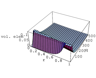
Figure 6: Two-dimensional marginal of the four-dimensional extended Husimi volume element (21)

Continuing with our numerical methods, we obtain the interesting unimodal curve (Fig. 7) — the peak being near $q=3.59782$, with a value there of 0.448488. This portrays the  one-dimensional marginal Husimi volume element over $q$ (cf. Fig. 4).

Figure 7: One-dimensional marginal over $q$ of the four-dimensional extended Husimi volume element (21). There is a peak near $q=3.59782$

In Fig. 8 we show the (quite difficult-to-compute) one-dimensional marginal over $r$ (cf. Fig. 5). (It appears the upturn near $r=1$ may be simply a numerical artifact. The difficulty consists in that, in some sense, we have to repeatedly perform numerical integrations using results of other numerical integrations. It would be of interest to see how the curve changes as the range of $q\in[\frac{1}{2},500]$ is modified.)

Figure 8: One-dimensional marginal over $r$ of the four-dimensional extended Husimi volume element (21). The upturn near $r=1$ may be due to (hard-to-avoid) numerical inaccuracy.

IV.1 Three-dimensional metric

For the case $q=1$, the (unextended) three-dimensional Fisher information metric over the family of Husimi distributions takes the form (Slater, , eq. (2))

$$ds_{F}(\rho,\rho+d\rho)^{2}=\frac{-2r-\log(\frac{1-r}{1+r})}{2r^{3}}dr^{2}+\Big{(}(1+r)f_{F}(\frac{1-r}{1+r})\Big{)}^{-1}dn^{2}.$$ (19)

Here,

$$f_{F}(t)=\frac{(t-1)^{3}}{t^{2}-2t\log{t}-1},$$ (20)

which is the limiting case ($q\to 1$) of (11). To normalize the volume element of this metric (19) to a prior probability distribution ($p_{F}$), we divide it by 1.39350989 Slater .

IV.2 Four-dimensional metric

In the extended (four-dimensional) case (cf. (14)), after having set $q=1$, we have,

$$ds_{F_{q=1}}(\rho,\rho+d\rho)^{2}=\Big{(}\frac{1}{4}-\frac{(-1+r^{2})^{2}\log^{2}{W}}{16r^{2}}\Big{)}dq^{2}$$ (21)

$$+\frac{2r-(-1+r^{2})\log{W}}{2r^{2}}dqdr+ds_{F}(\rho,\rho+d\rho)^{2}.$$

(So, the metric tensor here, in the same manner as in the untruncated extended Bures case (10), is not fully diagonal. We do not truncate the $q$-extended Fisher information metric (21) in any of our analyses.) To normalize its (non-null) volume element to a prior probability distribution ($p_{F_{q=1}}$) over the Bloch sphere, we must divide by 0.24559293.

V Comparative Noninformativity Analysis

We have that $S_{KL}(p_{F}||p_{F_{q=1}})=0.229666$ and $S_{KL}(p_{F_{q=1}}||p_{F})=0.170145$. Further, using the likelihood (16), based on six hypothetical measurements to generate posteriors, we obtain $S_{KL}(post_{F},p_{F_{q=1}})=0.70766$ and $S_{KL}(post_{F_{q=1}}||p_{F})=0.0641738$. So, the comparative noninformativity test, which was initially developed by Clarke Clarke (1996), leads us to a firm conclusion that the four-dimensional-based probability distribution $p_{F_{q=1}}$ is more noninformative in nature than the three-dimensional-based $p_{F}$.

Additionally, $S_{KL}(p_{B}||p_{F_{q=1}})=0.148269$ and $S_{KL}(p_{F_{q=1}}||p_{B})=0.0989669$. These are converted, respectively, to 0.283218 and 0.0842879 if we replace the first arguments of the two relative entropy functionals by posterior distributions based on the (formal) square root ($L(x,y,z)^{\frac{1}{2}}$) of the likelihood function (16). Thus, we can conclude that $p_{F_{q=1}}$ is also more noninformative than $p_{B}$.

Further, $S_{KL}(p_{B_{q=1}trunc}||p_{F_{q=1}})=0.105463$ and $S_{KL}(p_{F_{q=1}}||p_{B_{q=1}trunc})=0.0914175$. Again, using the formal square root ($L(x,y,z)^{\frac{1}{2}}$) of the likelihood, we obtain changes, respectively, to 0.245602 and 0.0408236. So, our conclusion here is that $p_{F_{q=1}}$ is also more noninformative than $p_{B_{q=1}trunc}$. We already know from Slater that $p_{B}$ is considerably more noninformative than $p_{F}$.

Continuing along these lines, $S_{KL}(p_{B_{q=1}trunc}||p_{F})=0.0191948$ and $S_{KL}(p_{F}||p_{B_{q=1}trunc})=0.0234599$ (so the two distributions are relatively close to one another). Using ($L(x,y,z)^{\frac{1}{2}}$) to generate posterior distributions, the first statistic is altered (slightly decreased) to 0.0143147, while the second statistic jumps to 0.1047772.

So, assembling these several relative entropy statistics, we have the previously indicated ordering of the four priors (1). (The conclusions of the comparative noninformativity test appear to be transitive in nature, although I can cite no explicit theorem to that effect.)

V.1 Relation to Srednicki’s Criterion for Priors

In Fig. 1, we show the one-dimensional marginal probabilities of the four prior probabilities over the radial coordinate $r$ in the near-to-pure-state range $r\in[.995,1]$. The dominance ordering in this plot fully complies with that (1) found by the information-theoretic-based comparative noninformativity test. (We note that this ordering is not simply reversed near to the fully mixed state [$r=0$].) Conjecturally, this could be seen as a specific case of some (yet unproven) theorem — perhaps utilizing the convexity and decreasing-under-positive-mappings properties (Ohya and Petz, 2004, p. 35) of the relative entropy functional.

So, the information-theoretic (comparative-noninformativity) test appears to incorporate Srednicki’s criterion of “biasedness to pure states” Srednicki (2005). (Of course, it would be interesting to test the consistency between the comparative noninformativity test and Srednicki’s criterion with a larger number of priors, as well as in higher-dimensional quantum settings (cf. Slater (1996b)).) Srednicki does not explicitly observe that increasing biasedness to pure states corresponds to increasing noninformativity. He asserts that “we must decide how biased we are towards pure states”.

Srednicki focused on two possible priors. One was the uniform distribution over the Bloch sphere (unit ball). In (Slater, 1998, sec. 2.2), we had concluded that this distribution was less noninformative than $p_{B}$, in full agreement with contemporaneous work of Hall Hall (1998). The second prior (“the Feynman measure”), which Srednicki points out is less biased to the pure states than the uniform distribution, was discussed in Slater (2000b). Neither of the two priors analyzed by Srednicki corresponds to the normalized volume element of a monotone metric Slater (1998, 2000b).

VI $q$-Extended Inference

In the setting of the $q$-parameterized escort density matrices (9), the factor $\frac{1-z^{2}}{4}$ in the likelihood (16), giving the probability (in the standard three-dimensional Bloch sphere setting) of one spin-up and one spin-down being measured in the $z$-direction, would be replaced by

$$L_{q}(z)=\frac{r^{2}(1+W^{q})^{2}-(-1+W^{q})^{2}z^{2}}{4r^{2}(1+W^{q})^{2}},$$ (22)

and similarly for the $x$- and $y$-directions. (For $q=1$, we recover $\frac{1-z^{2}}{4}$.)

It would be interesting to ascertain if the volume elements of the extended four-dimensional (truncated) Bures and Husimi metrics ((10) and (21)) could be integrated over the product of the Bloch sphere and $q\in[\frac{1}{2},\infty]$ and normalized to (prior) probability distributions. Then, using likelihoods incorporating the form (22), one could conduct the comparative noninformativity test in a four-dimensional setting, rather than only the three-dimensional one employed throughout this study. It turns out, however, that the three-fold integral — holding $q$ fixed — of the truncated volume element of (10) over the Bloch sphere is given by our formula (12). Therefore, the four-fold integral of the one-dimensional marginal over the indicated product region with $q\in[\frac{1}{2},\infty]$ must diverge. So, to achieve a proper probability distribution one would have to truncate $q$ above a certain value.

Continuing along these lines, we omitted $q$ above 500 (and below $q=\frac{1}{2}$) and normalized the volume element of the (truncated) extended Bures metric to a proper probability distribution. Then, the information gain with respect to such a prior, using $L_{q}(z)$, is 0.0597923 nats of information, while a single up or down measurement yields 0.134651 nats, and two measurements along the same axis giving the same outcome leads to an information gain of 0.349601. The analogous three (slightly larger) statistics, working in the unextended framework (where $q$ does not explicitly enter, and is implicitly understood to equal 1), using $p_{B}$ as prior, are, respectively, $\frac{7}{6}-\log{3}\approx 0.0680544$, and

$$\frac{8\,_{p}F_{q}(\{\frac{1}{2},1,2\},\{\frac{3}{2},\frac{5}{2}\},1)-\pi\,\left(-5+\log(64)\right)-6-12\,K}{6\,\pi}\approx 0.140186,$$ (23)

(where ${}_{p}F_{q}$ denotes a generalized hypergeometric function and $K\approx 0.915965594177$ is Catalan’s constant) and $\frac{59}{30}-\log{5}\approx 0.357229$. (We encountered numerical difficulties using Mathematica in attempting to extend these analyses to measurements conducted in more than one direction, unless we restricted $q$ to a range no larger than on the order of 10.)

One might also consider the possible relevance of $q$-analogs of the Clarke comparative noninformativity test, using $q$-relative entropy (Kullback-Leibler) divergence Johal (1998); Suyari (2002).

VII $q$-Extended Bures Metric for Higher-Dimensional Quantum Scenarios

VII.1 Four-Variable $3\times 3$ Density Matrices

In Slater (1996b), we considered an extension of the $2\times 2$ density matrices (4) to the $3\times 3$ form (by incorporating an additional parameter $v$)

$$\rho=\frac{1}{2}\left(\begin{array}[]{ccc}v+z&0&x-iy\\ 0&2-2v&0\\ x+iy&0&v-z\\ \end{array}\right),\hskip 36.135ptr^{2}=x^{2}+y^{2}+z^{2}\leq v^{2};\hskip 21.68121pt0\leq v\leq 1,$$ (24)

The Bures metric was found there to take the form

$$d_{B_{n=3}}(\rho,\rho+d\rho)^{2}=\frac{1}{4}\Big{(}\frac{r^{2}-v}{(1-v)(r^{2}-v^{2})}dv^{2}+\frac{r}{r^{2}-v^{2}}dvdr++\frac{v}{v^{2}-r^{2}}dr^{2}+\frac{1}{v}dn^{2}\Big{)}.$$ (25)

(So, the tangential component is independent of $r$, as with (6) (cf. Hall (1998)).) Normalizing the volume element of (25), we obtain the prior probability distribution (Slater, 1996b, eq. (18))

$$p_{B_{n=3}}=\frac{3r^{2}\sin{\theta_{1}}}{4\pi^{2}v\sqrt{1-v}\sqrt{v^{2}-r^{2}}}.$$ (26)

We have calculated that the (five-dimensional) $q$-extension of this metric has a tangential component of the form

$$\frac{{\left({\left(-r+v\right)}^{q}-{\left(r+v\right)}^{q}\right)}^{2}}{4\,r^{2}\,\left({\left(-r+v\right)}^{q}+{\left(r+v\right)}^{q}\right)\,\left({\left(2-2\,v\right)}^{q}+{\left(-r+v\right)}^{q}+{\left(r+v\right)}^{q}\right)},$$ (27)

but have not yet been able to derive simple forms for the other entries of this metric tensor.

Numerical tests appear to indicate that the volume element of this $q$-extended Bures metric tensor is (also) identically zero.

VII.2 Abe-Rajagopal Two-Qubit States

Since our first two attempts above to extend the Bures metric from an $n$-dimensional setting to an $(n+1)$-dimensional framework, by embedding the $q$ order parameter, have yielded metrics (one of them being (10)) with zero volume elements, we were curious as to whether or not we could obtain, in some other quantum context, a nondegenerate $q$-extension of the Bures metric. In this regard, we turned our attention to the paper, “Quantum entanglement inferred by the principle of maximum nonadditive entropy” of Abe and Rajagopal Abe and Rajagopal (1999) (cf. (Tsallis et al., 2001, eq. (14))).

Their principal object of study is a $4\times 4$ density matrix (Abe and Rajagopal, 1999, eq. (32)), being ostensibly parameterized by three variables, the order (nonadditivity) parameter $q$, the $q$-expected value $b_{q}$ of the Bell-CHSH observable and its dispersion $\sigma_{q}^{2}$. (Two of the four eigenvalues of the density matrix are always equal.)

We applied the Hübner formula (3) for the Bures metric to this family of $4\times 4$ density matrices, considering $q$ as a freely-varying parameter, along with $b_{q}$ and $\sigma_{q}^{2}$. Computing the $3\times 3$ Bures metric tensor, and then setting $q=1$, we obtain the metric

$$ds_{AbeRaj_{q=1}}(\rho,\rho+d\rho)^{2}=\frac{c}{1024}dq^{2}+$$ (28)

$$\frac{\log(-2\,{\sqrt{2}}\,{b_{q}}+{{{\sigma}_{q}}}^{2})-\log(2\,{\sqrt{2}}\,{b_{q}}+{{{\sigma}_{q}}}^{2})}{8\,{\sqrt{2}}}dqdb_{q}+$$

$$\frac{2\,\log(8-{{{\sigma}_{q}}}^{2})-\log(-2\,{\sqrt{2}}\,{b_{q}}+{{{\sigma}_{q}}}^{2})-\log(2\,{\sqrt{2}}\,{b_{q}}+{{{\sigma}_{q}}}^{2})}{32}dqd\sigma_{q}^{2}+$$

$$\frac{\sigma_{q}^{2}}{-32b_{q}^{2}+4(\sigma_{q}^{2})^{2}}(db_{q})^{2}+\frac{b_{q}}{16b_{q}^{2}-2(\sigma_{q}^{2})^{2}}db_{q}d\sigma_{q}^{2}+\frac{b_{q}^{2}-\sigma_{q}^{2}}{4(-8+\sigma_{q}^{2})(-8b_{q}^{2}+(\sigma_{q}^{2})^{2})}(d\sigma_{q}^{2})^{2}.$$

Here, we have

$$c=-4\,{\log(8-{{{\sigma}_{q}}}^{2})}^{2}\,{{{\sigma}_{q}}}^{2}\,\left(-8+{{{\sigma}_{q}}}^{2}\right)+2\,\log(-2\,{\sqrt{2}}\,{b_{q}}+{{{\sigma}_{q}}}^{2})\,\log(2\,{\sqrt{2}}\,{b_{q}}+{{{\sigma}_{q}}}^{2})\,\left(8\,{{b_{q}}}^{2}-{{{{\sigma}}_{q}}}^{4}\right)$$ (29)

$$-{\log(-2\,{\sqrt{2}}\,{b_{q}}+{{{\sigma}_{q}}}^{2})}^{2}\,\left(8\,{{b_{q}}}^{2}+{{{\sigma}_{q}}}^{2}\,\left(-16+{{{\sigma}_{q}}}^{2}\right)-4\,{\sqrt{2}}\,{b_{q}}\,\left(-8+{{{\sigma}_{q}}}^{2}\right)\right)$$

$$-{\log(2\,{\sqrt{2}}\,{b_{q}}+{{{\sigma}_{q}}}^{2})}^{2}\,\left(8\,{{b_{q}}}^{2}+{{{\sigma}_{q}}}^{2}\,\left(-16+{{{\sigma}_{q}}}^{2}\right)+4\,{\sqrt{2}}\,{b_{q}}\,\left(-8+{{{\sigma}_{q}}}^{2}\right)\right)+$$

$$4\,\log(8-{{{\sigma}_{q}}}^{2})\,\left(-8+{{{{\sigma}}_{q}}}^{2}\right)\,\left(\log(-2\,{\sqrt{2}}\,{b_{q}}+{{{\sigma}_{q}}}^{2})\,\left(-2\,{\sqrt{2}}\,{b_{q}}+{{{{\sigma}}_{q}}}^{2}\right)+\log(2\,{\sqrt{2}}\,{b_{q}}+{{{\sigma}_{q}}}^{2})\,\left(2\,{\sqrt{2}}\,{b_{q}}+{{{{\sigma}}_{q}}}^{2}\right)\right).$$

Numerical computations indicate that the volume element of the metric $ds_{AbeRaj_{q}}(\rho,\rho+d\rho)^{2}$, for any value of $q$, is zero.

In the unextended (two-parameter) case, the nondegenerate volume element (with $q=1$) is

$$dV_{AbeRaj_{q=1}}=\frac{{\sqrt{-\left(\frac{1}{\left(-8+\sigma_{q}\right)\,\left(-8\,b_{q}^{2}+(\sigma_{q}^{2})^{2}\right)}\right)}}}{4}db_{q}d\sigma_{q}^{2}.$$ (30)

VII.2.1 $q$-Invariance of Bures Volumes of Separable and Separable and Nonseparable AR States

In Slater (2000c), it was asserted that for the cases $q=\frac{1}{2}$ and 1, the associated separability probabilities of the Abe-Rajagopal (AR) states were equal to the “silver mean”, that is, $\sqrt{2}-1\approx 0.414214$ (cf. Slater (2005a, b). We have reconfirmed these two probabilities, while also finding that the Bures volume of separable and nonseparable states is, in both these cases, equal to $\frac{\pi}{4}\approx 0.7853981634$. This also appears to be the Bures volume for all positive $q$, as indicated by the results obtained by numerical integration presented in Fig. 9.

Figure 9: Numerical integration estimates of the Bures volume of the (separable and nonseparable) AR two-qubit states, as a function of $q$. This volume is known to be $\frac{\pi}{4}\approx 0.7853981634$ for $q=\frac{1}{2}$ and 1 and appears to be so for all (positive) $q$.

The integrand employed (that is, the Bures volume element) was

$$dV_{AbeRaj}=16\sqrt{\frac{\left(8-\sigma_{q}\right)^{\frac{1}{q}-2}\left(\sigma_{q}-2\sqrt{2}b_{q}\right)^{\frac{1}{q}}\left(2\sqrt{2}b_{q}+\sigma_{q}\right)^{\frac{1}{q}}}{q^{4}\left(\sigma_{q}^{2}-8b_{q}^{2}\right)^{2}\left(2\left(8-\sigma_{q}\right)^{\frac{1}{q}}+\left(\sigma_{q}-2\sqrt{2}b_{q}\right)^{\frac{1}{q}}+\left(2\sqrt{2}b_{q}+\sigma_{q}\right)^{\frac{1}{q}}\right)^{3}}}db_{q}d\sigma_{q}^{2}.$$ (31)

It also appears (Fig. 10) that the Bures volume of the separable (only) AR-states is equal to $\frac{\pi(\sqrt{2}-1)}{4}\approx 0.325323$ for all positive $q$ and, thus, the separability probabilities (obtained by taking the ratios) are all simply $\sqrt{2}-1\approx 0.414214$ (that is, the “silver mean”). (The numerical integration employed to generate Fig. 10 is more challenging — due to the necessary imposition of the Peres separability criterion — than to create Fig. 9, so we could not obtain as many significant digits.)

Figure 10: Numerical integration estimates of the Bures volume of the separable A two-qubit states, as a function of $q$. This volume is known to be exactly $\frac{\pi(\sqrt{2}-1)}{4}\approx 0.325323$ for $q=\frac{1}{2}$ and 1 and appears to be so for all (positive) $q$.

These $q$-invariance results stand in interesting contrast to the emphasis of Abe and Rajagopal “that for $q>1$, indicating the subadditive feature of the Tsallis entropy, the entangled region is small and enlarges as one goes into the superadditive regime where $q<1$” (Abe and Rajagopal, 1999, p. 3464 and Fig. 1). But, in terms of the Bures metric (and others we will see below) the measure of the region does not change with $q$.

Using the Hilbert-Schmidt metric Życzkowski and Sommers (2003), rather than the Bures, we find that the volume of separable and nonseparable AR two-qubit states is equal to $\frac{1}{4\sqrt{2}}$ for both $q=\frac{1}{2}$ and 1 and the volume of separable states is equal to $\frac{1}{8\sqrt{2}}$ for both these values of $q$, so the corresponding Hilbert-Schmidt separability probabilities are simply $\frac{1}{2}$. (If we employ either the Wigner-Yanase [monotone] metric Gibilisco and Isola (2003) or the arithmetic average [monotone] metric Slater (2005b), then, for $q=1$, we obtain exactly the same [volume] results as using the Bures metric, and for $q=\frac{1}{2}$ — using numerical rather than symbolic methods in the Wigner-Yanase case — quite clearly the same also.) So, it certainly appears that the $q$-invariance of the total and separable volumes of the AR-states is metric-independent. Canosa and Rossignoli (Canosa and Rossignoli, 2002, p. 4) have noted that for the AR-states, the “final maximum entropy density is actually independent of the choice of $f$”, where $f$ is a smooth concave function.

The Bures separability probability (as well as that based on the Wigner-Yanase metric) of the (one-parameter) “Jaynes state” Horodecki et al. (1999); Rajagopal (1999), in which (unlike the AR-states) no constraint on the dispersion is present (and $q$ is implicitly equal to 1) , is $\frac{2\,\arcsin({\sqrt{2}}-1)}{\pi}\approx 0.271887$. (Again, note the presence of the silver mean — and implicitly in the very next formula.) The Hilbert-Schmidt separability probability is

$$\frac{\sinh^{-1}\left(2-\sqrt{2}\right)+\text{Root}\left[\text{$\#$1}^{4}-148\text{$\#$1}^{2}+68\&,3\right]}{\sqrt{6}+\sinh^{-1}\left(\sqrt{2}\right)}\approx 0.343602.$$ (32)

To convert from the AR two-qubit density matrix for $q=1$ to that for $q=\frac{1}{2}$, we merely have to perform the transformation

$$\left\{\sigma_{1}^{2}\to\frac{4\left(8b_{\frac{1}{2}}^{2}+{(\sigma^{2}_{\frac{1}{2}})}^{2}\right)}{4b_{\frac{1}{2}}^{2}+{(\sigma^{2}_{\frac{1}{2}})}^{2}-8{\sigma^{2}_{\frac{1}{2}}}+32},b_{1}\to\frac{8b_{\frac{1}{2}}{\sigma^{2}_{\frac{1}{2}}}}{4b_{\frac{1}{2}}^{2}+{(\sigma^{2}_{\frac{1}{2}})}^{2}-8{\sigma^{2}_{\frac{1}{2}}}+32}\right\}.$$ (33)

Presumably, there is a (more complicated, in general) transformation between AR-states for any pair of distinct values of $q$. So, in retrospect, the $q$-invariance of the (Bures, Hilbert-Schmidt, Wigner-Yanase and arithmetic average) metric volumes is not so surprising, since we are simply working within one family of two-parameter density matrices, the various $q$-manifestations of which can be obtained by suitable reparameterizations. Similarly, the null nature of the $q$-extended Bures metric for the AR-states can be seen in this light.

VII.2.2 Trivariate Jaynes state using generalized Bell-CHSH observables

It would be interesting to extend and analyze the AR-states based on modifications of the Bell-CHSH observable (cf. (Canosa and Rossignoli, 2005, sec. 3) Batle et al. (2002)). In fact, we pursued such a line of investigation, using

$$B_{\alpha}=2\sqrt{2}(|\Phi^{+}\rangle\langle\Phi^{+}|-\alpha|\Psi^{-}\rangle\langle\Psi^{-}|),$$ (34)

as the observable, where for $\alpha=1$, we recover the Bell-CHSH observable employed by Abe and Rajagopal (Abe and Rajagopal, 1999, eq. (6)) (cf. (Canosa and Rossignoli, 2005, eq. (15))). (We utilized the Jaynes maximum entropy strategy Horodecki et al. (1999), implicitly taking $q=1$ — so, most precisely, we are extending the model discussed by Rajagopal in Rajagopal (1999) to incorporate generalized Bell-CHSH observables or, alternatively, the Canosa-Rossignoli model to included the dispersion.) Then, the volume element of the Bures metric, considering $\alpha$ as a parameter, in addition to the expectation $b_{1}$ and the dispersion $\sigma_{1}$, was null. Considering, on the other hand, $\alpha$ to be simply a fixed constant, the bivariate Bures volume element was of the (non-null) form $\frac{1}{4}\sqrt{\frac{1}{C+D}}db_{1}d\sigma_{1}^{2}$, where

$$C=\left(8\alpha-\sigma_{1}^{2}\right)(\sigma_{1}^{2})^{2}-4\sqrt{2}(\alpha-1)b_{1}\left(\sigma_{1}^{2}-4\alpha\right)\sigma_{1}^{2}+$$ (35)

and

$$D=16\sqrt{2}(\alpha-1)\alpha b_{1}^{3}-8b_{1}^{2}\left(\left(\sigma_{1}^{2}+8\right)\alpha^{2}-3\sigma_{1}^{2}\alpha+\sigma_{1}^{2}\right).$$

For $\alpha=1$, we recover (30), so the associated Bures separability probability is the silver mean. For $\alpha=1$, using the HS-metric now, the total volume of states is $\frac{1}{4\sqrt{2}}$ and that of the separable states is $\frac{1}{8\sqrt{2}}$, so the HS separability probability is simply $\frac{1}{2}$.

For the case $\alpha=2$, we obtained a result of 0.35368 for the Bures volume of separable and nonseparable states, and 0.2000322 for the Bures volume of only separable states, yielding a separability probability of 0.566392. The comparable results for the Hilbert-Schmidt case (the volume element — independent of $b_{q}$ and $\sigma_{q}^{2}$ — being $\frac{1}{32\alpha(1+\alpha)}db_{q}d\sigma_{q}^{2}$) were $\frac{1}{12\sqrt{2}}$ and $\frac{5}{96\sqrt{2}}$, with a separability probability of $\frac{5}{8}$.

Exact integration, then, gave the HS volume of separable and nonseparable states to equal, in general, $\frac{1}{2\sqrt{2}(\alpha+\alpha^{2})}$, and that of the separable states — but only for $\alpha\geq 1$ — to be $\frac{3\alpha-1}{8\sqrt{2}\alpha^{2}(1+\alpha)}$, so the Hilbert-Schmidt separability probability for $\alpha\geq 1$ is simply equal to $\frac{3}{4}-\frac{1}{4\alpha}$. For $\alpha=\frac{1}{2}$, the HS separability probability appeared to be $\frac{37}{64}\approx 0.578125$.

Then, using the integration over implicitly defined regions feature new to Mathematica 5.1, we were able to obtain the HS separable volumes, for all (real) values of $\alpha$,

$$\left(\begin{array}[]{ll}-\frac{1}{8\sqrt{2}}&-1<\alpha<0\\ \frac{5}{16\sqrt{2}}&\alpha=-\sqrt{2}\\ \frac{1}{32}\left(5\sqrt{2}-\sqrt{10}\right)&\alpha=-\frac{1}{2}+\frac{\sqrt{5}}{2}\\ \frac{1}{16}\left(2\sqrt{2}-\sqrt{2}\alpha\right)&0<\alpha<-\frac{1}{2}+\frac{\sqrt{5}}{2}\lor-\frac{1}{2}+\frac{\sqrt{5}}{2}<\alpha<1\\ \frac{3\sqrt{2}\alpha-\sqrt{2}}{16\alpha^{2}(\alpha+1)}&\alpha\geq 1\\ \frac{3\sqrt{2}\alpha^{2}+\sqrt{2}}{16\alpha^{2}\left(\alpha^{2}-1\right)}&\alpha\leq-\sqrt{3}\\ \frac{-\sqrt{2}\alpha^{4}+5\sqrt{2}\alpha^{2}-\sqrt{2}}{16\alpha^{2}}&-\sqrt{2}<\alpha<-1\lor-\sqrt{3}<\alpha<-\sqrt{2},\end{array}\right)$$ (36)

and, dividing by the total HS volume ($\frac{1}{2\sqrt{2}(\alpha+\alpha^{2})}$), the HS separability probability results,

$$\begin{cases}-\frac{1}{4}\alpha(\alpha+1)&-1<\alpha<0\\ \frac{5}{8}\alpha(\alpha+1)&\alpha+\sqrt{2}=0\\ -\frac{1}{8}\left(-5+\sqrt{5}\right)\alpha(\alpha+1)&2\alpha+1=\sqrt{5}\\ -\frac{1}{4}(\alpha-2)\alpha(\alpha+1)&0<\alpha<\frac{1}{2}\left(-1+\sqrt{5}\right)\lor\frac{1}{2}\left(-1+\sqrt{5}\right)<\alpha<1\\ \frac{3}{4}-\frac{1}{4\alpha}&\alpha\geq 1\\ -\frac{1}{4\alpha}+\frac{3}{4}+\frac{1}{\alpha-1}&\alpha+\sqrt{3}\leq 0\\ -\frac{(\alpha+1)\left(\alpha^{4}-5\alpha^{2}+1\right)}{4\alpha}&-\sqrt{2}<\alpha<-1\lor-\sqrt{3}<\alpha<-\sqrt{2}\end{cases}$$ (37)

In Fig. 11, we plot these rather interesting/intricate results.

Figure 11: Separability probabilities (37) based on the Hilbert-Schmidt metric, as a function of the parameter $\alpha$, for the new class of trivariate Jaynes states employing generalized Bell, Clauser, Horne, Shimony, Holt (Bell-CHSH) observables (34)

The separability probabilities are zero at the isolated points $\alpha=-1,0$. For $\alpha\to\pm\infty$, a maximum of $\frac{3}{4}$ is approached. We also see that the “golden ratio” (or “golden mean”) Livio (2002); Markowsky (2004) [or its inverse, depending upon the definition], $\frac{\sqrt{5}-1}{2}$, enters into delineating the different segments over which the separability probabilities take different functional forms. (It would seem plausible, although we have not conducted a full, detailed analysis that the points at which the functional forms change, correspond to separability constraints passing from inactive to active roles, and vice versa.)

Fake entanglement is avoided in this three-parameter model (Canosa and Rossignoli, 2005, p. 128) (Canosa and Rossignoli, 2002, p. 4). It did not appear feasible to directly expand the trivariate $(b_{q},\sigma_{q}^{2},\alpha)$ scenario just investigated to a quadrivariate one.

VII.2.3 Bivariate Jaynes state using generalized Bell-CHSH observables

Let us, however, consider a related bivariate (Canosa-Rossignoli-type (Canosa and Rossignoli, 2005, p. 126)) model, in which we set $\sigma_{1}^{2}=4(1+\frac{b_{1}^{2}}{8})$, the dispersion in the single constraint case (Rajagopal, 1999, eq. (13)). Then, the HS separability probabilities take the form (the HS volume here being $\frac{2\sqrt{3\alpha^{4}-2\alpha^{2}+3}}{4\alpha^{2}+4\alpha}$),

$$\begin{cases}-\alpha-1&\frac{1}{3}\left(1-2\sqrt{7}\right)<\alpha<-1\\ \sqrt{(\alpha-2)\alpha}-\sqrt{\alpha(\alpha+1)}-1&3\alpha+2\sqrt{7}\leq 1\\ \sqrt{\alpha(\alpha+1)}-\alpha&2\alpha+1\geq\sqrt{5}\\ -\alpha+2\sqrt{\alpha(\alpha+1)}-1&\frac{1}{3}<\alpha<\frac{1}{2}\left(-1+\sqrt{5}\right).\end{cases}$$ (38)

We represent this in Fig. 12.

Figure 12: Separability probabilities (38) based on the Hilbert-Schmidt metric, as a function of the parameter $\alpha$, for the (Canosa-Rossignoli) class of bivariate Jaynes states employing generalized Bell, Clauser, Horne, Shimony, Holt (Bell-CHSH) observables (34). The variance $\sigma_{1}^{2}$ has been set to its value $4(1+\frac{b_{1}^{2}}{8})$ in the single constraint (Horodecki) case

In the $\pm\infty$ limit, the separability probability approaches $\frac{1}{2}$. The HS separability probability is zero in the interval $\alpha\in[-1,\frac{1}{3}]$. The point $\alpha=1$ corresponds to the use of the standard (ungeneralized) Bell-CHSH observable ($B_{1}$), and to the one-constraint Horodecki model Horodecki et al. (1999). We can see that the associated HS separability probability is the silver mean.

VII.3 Tsallis-Lloyd-Baranger Two-Qubit States

Tsallis, Lloyd and Baranger have considered a scenario in which the probabilities of being in either one of the four states of the Bell basis is given in the form $\frac{(1-x)}{4},\frac{(1-y)}{4},\frac{(1-z)}{4}$ and $\frac{(1+x+y+z)}{4}$ Tsallis et al. (2001). (The feasible points $(x,y,z)$ lie in a certain tetrahedron (Tsallis et al., 2001, Fig. 3).) They also embed their three-parameter (two-qubit) $4\times 4$ density matrix (Tsallis et al., 2001, eq. (12)) into an (unnormalized) four-parameter $4\times 4$ density matrix (Tsallis et al., 2001, eq. (14)) by introducing the $q$-parameter.

Upon its normalization and application of the Hübner formula (3), we obtained the corresponding Bures metric, the volume element of which, in a numerical investigation, appeared to be zero, in this four-parameter extended case. So, we have, to this point, yet to find any nondegenerate $q$-extension of the Bures metric (if one is so possible).

In the unextended three-parameter case, if we employ new coordinates of the form,

$$x=1-4\cos{\theta_{1}},y=1-4\sin{\theta_{1}}\cos{\theta_{2}},z=1-4\sin{\theta_{1}}\sin{\theta_{2}}\cos{\theta_{3}},$$ (39)

then we have simply

$$d_{TLB}(\rho,\rho+d\rho)^{2}=d\theta_{1}^{2}+\sin{\theta_{1}}^{2}d\theta_{2}^{2}+\sin{\theta_{1}}^{2}\sin{\theta_{2}}^{2}d\theta_{3}^{2},$$ (40)

that is, the uniform metric on the 3-sphere.

The Bures volume of the (separable and nonseparable) TLB-states is $\frac{\pi^{2}}{8}$, while the Bures volume of just the separable states themselves is (thanks to a challenging computation — involving a cylindrical algebraic decomposition [cad] Brown (2001) — performed by M. Trott) $\frac{\pi(4-\pi)}{8}$. (The separable states comprise the cube $x,y,z\in[-1,\frac{1}{3}]$.) Thus, the Bures separability probability Slater (2000c, 2005a, 2005b) of the TLB-states is (quite elegantly) $\frac{4-\pi}{\pi}\approx 0.27324$.

For the Hilbert-Schmidt metric, the volume of the TLB (separable and nonseparable) states is $\frac{1}{6\sqrt{2}}$ and that of the separable states, $\frac{1}{12\sqrt{2}}$, so the HS separability probability is $\frac{1}{2}$.

VIII Rajagopal-Abe Metric

We also investigated the possible application of the “generalized ’metric” (based on the $q$-Kullback-Leibler entropy) (Rajagopal and Abe, 1999, eq. (16)) to the two-level quantum systems (4) — and seeing how it pertains to the family of quantum monotone metrics Petz and Sudár (1996). For the case $q=1$ (which should reduce to the Kullback-Leibler symmetrized divergence (Rajagopal and Abe, 1999, eq. (6)), our calculations yielded that the diagonal elements of the “metric” take the form

$$\frac{1}{2}\Big{(}-\log{(-\frac{r}{2+r})}+\log{W}\Big{)}dr^{2}-\frac{1}{4}r(3+\cos{2\theta_{1}}+2\sin{2\theta_{1}})\log{W}d\theta_{1}^{2}$$ (41)

$$-\frac{1}{4}r(3+\cos{2\theta_{2}}+2\sin{2\theta_{2}})\log{W}\sin^{2}{\theta_{1}}d\theta_{1}^{2},$$

where, as we recall, $W=\frac{1-r}{1+r}$. So, it clearly can not possess the form required of a quantum monotone metric (cf. Sec. III.1). However, when we attempted to implement equation (6) of (Rajagopal and Abe (1999)), bypassing the $q$-framework, we obtained for the (presumably same?) metric

$$\frac{1}{1-r^{2}}dr^{2}-\frac{1}{2r}\log{W}dn^{2},$$ (42)

which does not appear to correspond to a monotone metric.

IX Concluding Remarks

Naudts Naudts introduced the concept of a $\phi$-exponential family of density operators $\rho_{\theta}$ (for which the obvious example is $\phi(u)=u^{q}$). He showed that the $\phi$-exponential family of density operators, together with a family of escort density operators, optimizes a generalized version of the well-known Cramér-Rao lower bound. He assumes that certain Hamiltonians are two-by-two commuting. Therefore, the quantum information manifold $(\rho_{\theta})_{\theta}$ is abelian, which “is clearly too restrictive for a fully quantum-mechanical theory”. He suggests further work to remove this restriction.

Abe regarded the order of the escort distribution $q$ as a parameter Abe (2003). He studied the geometric structure of the one-parameter family of escort distributions using the Kullback divergence, and showed that the Fisher metric is given in terms of the generalized bit variance, which measures fluctuations of the crowding index of a multifractal.