Asymmetries in symmetric quantum walks on two-dimensional networks

Abstract

We study numerically the behavior of continuous-time quantum walks over networks which are topologically equivalent to square lattices. On short time scales, when placing the initial excitation at a corner of the network, we observe a fast, directed transport through the network to the opposite corner. This transport is not ballistic in nature, but rather produced by quantum mechanical interference. In the long time limit, certain walks show an asymmetric limiting probability distribution; this feature depends on the starting site and, remarkably, on the precise size of the network. The limiting probability distributions show patterns which are correlated with the initial condition. This might have consequences for the application of continuous time quantum walk algorithms.

I Introduction

The study of quantum mechanical extensions of classical transport processes has witnessed a considerable growth over the last decade, with much attention being given to quantum information and the application of transport processes in potential quantum computers Nielsen and Chuang (2000). This led to the development of several quantum algorithms specifically designed for these quantum computers. Among these algorithms are the so-called quantum walks, see for instance Shenvi et al. (2003); Childs and Goldstone (2004), which are the analog of the classical random walks Aharonov et al. (1993); Farhi and Gutmann (1998), for an overview see Kempe (2003).

Such quantum walks have been studied in different situations. For instance, it was shown that continuous-time quantum walks can cause a remarkable speed-up of transport through certain graphs Childs et al. (2002), a feature which is not universal, as discussed in Ref. Mülken and Blumen (2005a), where it was shown that quantum transport can also become much slower than the classical one, depending on the initial conditions. Another variant of the quantum walk, the quantum mulitbaker map, was shown to exhibit a crossover from classical to quantal behavior with time, where the crossover time is given by the inverse of Planck’s constant Wójcik and Dorfman (2002, 2003).

For simple structures these quantum walks are directly related to well known problems in solid state physics. Thus, methods used in solid state physics can easily be applied to quantum walks. For instance, walks on one-dimensional lattice with periodic boundary conditions are readily treated by a Bloch ansatz Mülken and Blumen (2005b); Ziman (1972); Kittel (1986).

Here, we study quantum walks on two-dimensional networks. We focus on structures topologically equivalent to square lattices. For these we evaluate the transition probabilities between different nodes of the finite networks and compare these to the Bloch solutions. As we are going to show, these transition probabilities display odd, unexpected features.

The paper is organized as follows: In Sec.II we briefly review the properties of continuous time quantum walks and the Bloch ansatz. The time dependent transition probabilities between the nodes of the network are presented in Sec.III. We conclude with a summary of results in Sec.IV.

II Continuous time quantum walks

In quantum information theory, qubits on a graph are used to define the quantum analog of a random walk. There is a discrete Aharonov et al. (1993) and a continuous-time Farhi and Gutmann (1998) version. However, distinct from classical physics, these two are not equivalent to each other. Here, we will focus on continuous-time quantum walks on networks.

II.1 Continuous time quantum walks on graphs

We consider two-dimensional graphs, topologically equivalent to finite, square lattices of side length $N$. In this way the nodes of the graph are connected in a very regular manner. In general, to every graph there corresponds a discrete Laplace operator, sometimes called the adjacency or connectivity matrix ${\bf A}=(A_{\boldsymbol{ij}})$, defined by letting the non-diagonal elements $A_{\boldsymbol{ij}}$ equal $-1$ if nodes $\boldsymbol{i}$ and $\boldsymbol{j}$ are connected by a bond and $0$ otherwise. The diagonal element $A_{\boldsymbol{ii}}$ is given by the number of bonds which exit from node $\boldsymbol{i}$, i.e., $A_{\boldsymbol{ii}}$ equals the functionality $f_{\boldsymbol{i}}$ of the node. Thus, in our case we have $f_{\boldsymbol{i}}=2$ if node $\boldsymbol{i}$ is located at a corner of the square, $f_{\boldsymbol{i}}=3$ if the node is located along an edge (and is not a corner node), and $f_{\boldsymbol{i}}=4$ otherwise.

Classically, continuous-time random walks (CTRWs) are described by the master equation Weiss (1994); van Kampen (1990)

$$\frac{d}{dt}p_{\boldsymbol{k,j}}(t)=\sum_{l}T_{\boldsymbol{kl}}\ p_{\boldsymbol{l,j}}(t),$$ (1)

where $p_{\boldsymbol{k,j}}(t)$ is the conditional probability to find the walker at time $t$ at node $\boldsymbol{k}$ when starting at time $0$ at node $\boldsymbol{j}$. We assume an unbiased CTRW such that the transmission rate $\gamma$ of all bonds are equal. Then the transfer matrix of the walk, ${\bf T}=(T_{\boldsymbol{kj}})$, is related to the adjacency matrix by ${\bf T}=-\gamma{\bf A}$. Formally, Eq.(1) is solved by

$$p_{\boldsymbol{k,j}}(t)=\langle\boldsymbol{k}|e^{{\bf T}t}|\boldsymbol{j}\rangle.$$ (2)

The quantum mechanical extension of a CTRW, the continuous-time quantum walk (CTQW), is now defined by identifying the Hamiltonian of the system with the (classical) transfer operator, ${\bf H}=-{\bf T}$, Farhi and Gutmann (1998); Childs et al. (2002); Mülken and Blumen (2005a). However, there is no unique way of defining a CTQW. As mentioned in Childs and Goldstone (2004), there is some freedom in defining the diagonal elements of the Hamiltonian for a certain graph. A requirement for the CTQW is that ${\bf H}$ define a unitary process, whereas classically the CTRW is a probability conserving Markov processes, which requires $\sum_{\boldsymbol{k}}T_{\boldsymbol{kj}}=0$. As mentioned in Childs and Goldstone (2004), for regular networks, where all nodes have the same functionality, different choices of the Hamiltonian give rise to the same quantum dynamics. Nevertheless, in what follows we directly identify the Hamiltonian with the transfer operator since some of the networks we consider are non-regular.

In the spirit of a localized orbital picture we now introduce the states $|\boldsymbol{j}\rangle$ which are localized at the nodes $\boldsymbol{j}$ of the graph, requiring in an obvious notation that $\langle\boldsymbol{k}|\boldsymbol{j}\rangle=\delta_{\boldsymbol{k,j}}$ and that $\sum_{\boldsymbol{j}}|\boldsymbol{j}\rangle\langle\boldsymbol{j}|=\boldsymbol{1}$ where $\boldsymbol{1}$ is the identity operator. Under these conditions the Schrödinger equation (SE) reads

$$i\frac{d}{dt}|\boldsymbol{j}\rangle={\bf H}|\boldsymbol{j}\rangle,$$ (3)

where we set $\hbar=1$. Starting at time $t_{0}$ from the state $|\boldsymbol{j}\rangle$ the system evolves as ${\bf U}(t,t_{0})|\boldsymbol{j}\rangle$, where ${\bf U}(t,t_{0})=\exp(-i{\bf H}(t-t_{0}))$ is the quantum mechanical time evolution operator. Hence, the transition amplitude $\alpha_{\boldsymbol{k,j}}(t)$ from state $|\boldsymbol{j}\rangle$ at time $0$ to state $|\boldsymbol{k}\rangle$ at time $t$ is

$$\alpha_{\boldsymbol{k,j}}(t)=\langle\boldsymbol{k}|e^{-i{\bf H}t}|\boldsymbol{j}\rangle.$$ (4)

With Eq.(3) we find that

$$i\frac{d}{dt}\alpha_{\boldsymbol{k,j}}(t)=\sum_{l}H_{\boldsymbol{kl}}\alpha_{\boldsymbol{l,j}}(t).$$ (5)

We note that the main difference between Eq.(2) and Eq.(4) is that classically $\sum_{\boldsymbol{k}}p_{\boldsymbol{k,j}}(t)=1$, whereas quantum mechanically $\sum_{\boldsymbol{k}}|\alpha_{\boldsymbol{k,j}}(t)|^{2}=1$ holds.

For the full solution of Eqs.(1) and (5) all the eigenvalues and all the eigenvectors of ${\bf T}=-{\bf H}$ (or, equivalently, of ${\bf A}$) are needed. Let $\lambda_{n}$ denote the $n$th eigenvalue of ${\bf A}$ and ${\bf\Lambda}$ the corresponding eigenvalue matrix. Furthermore, let ${\bf Q}$ denote the matrix constructed from the orthonormalized eigenvectors of ${\bf A}$, so that ${\bf A}={\bf Q}{\bf\Lambda}{\bf Q}^{-1}$. Now the classical transition probability is given by

$$p_{\boldsymbol{k,j}}(t)=\langle\boldsymbol{k}|{\bf Q}e^{-t\gamma{\bf\Lambda}}{\bf Q}^{-1}|\boldsymbol{j}\rangle,$$ (6)

whereas the quantum mechanical transition probability is

$$\pi_{\boldsymbol{k,j}}(t)\equiv|\alpha_{\boldsymbol{k,j}}(t)|^{2}=|\langle\boldsymbol{k}|{\bf Q}e^{-it\gamma{\bf\Lambda}}{\bf Q}^{-1}|\boldsymbol{j}\rangle|^{2}.$$ (7)

The unitarity of the time evolution operator prevents the quantum mechanical transition probability from having a definite limit when $t\to\infty$. In order to compare the classical long time probability with the quantum mechanical one, one usually uses the limiting probability (LP), i.e., the long time average of $\pi_{\boldsymbol{k,j}}(t)$ Aharonov et al. (2001):

$$\chi_{\boldsymbol{k,j}}\equiv\lim_{T\to\infty}\frac{1}{T}\int_{0}^{T}dt\ \pi_{\boldsymbol{k,j}}(t).$$ (8)

II.2 Boundary conditions and the Bloch ansatz

Given that our two-dimensional structures have side length $N$, they contain $N^{2}$ nodes giving rise to $N^{2}$ basis states. We switch to a pair notation, by which we set $|\boldsymbol{j}\rangle=|j_{x},j_{y}\rangle$, where $j_{x}$ and $j_{y}$ are integer labels in the two directions, with $j_{x},j_{y}\in[1,N]$, see Fig.1. This labeling of the states is not to be confused with the labeling of the adjacency matrix. Note that capital bold letters denote matrices, while small bold letters denote the nodes and the states.

Figure 1: Sketch of a square network arranged as a regular lattice with the appropriate numbering of the nodes. Note that the actual geometrical realization can be much more flexible, see text for details.

We stop to recall a basic fact, namely that our matrix $\bf A$ does not necessarily imply that the structure we consider obey any kind of translational symmetry; in fact the symmetry of $\bf A$ is topological in nature, a fact well realized both in polymer physics Gurtovenko and Blumen (2002) and also in quantum chemistry Blumen and Merkel (1977), where the $\bf A$-matrices are fundamental in Hückel molecular orbital calculations Streitwieser (1961); McQuarrie (1983). Regular, translational invariant lattices are only one possible realization of the network structures we are facing here. The methods of solid state physics Ziman (1972); Kittel (1986) apply, however, even in our very general case.

The focus in solid state physics is on systems where Born - von Karman periodic boundary conditions (PBC) are assumed. Here, all transmission rates are taken to be equal. Hence, time is given in units of the inverse transmission rate $\gamma^{-1}$ or, equivalently, we set $\gamma=1$. Now, for an internal site of our network (not on an edge or in a corner), the Hamiltonian acting on a state $|\boldsymbol{j}\rangle=|j_{x},j_{y}\rangle$ reads

$${\bf H}|j_{x},j_{y}\rangle= 2|j_{x},j_{y}\rangle-|j_{x}+1,j_{y}\rangle-|j_{x}-1,j_{y}\rangle$$ (9)

$$+ 2|j_{x},j_{y}\rangle-|j_{x},j_{y}+1\rangle-|j_{x},j_{y}-1\rangle.$$

PBC extend this equation to all the sites of the network by interpreting every integer $j_{x}$ and $j_{y}$ to be taken modulus $N$. With this generalization, the time independent SE

$${\bf H}|\Psi_{\boldsymbol{\theta}}\rangle=E_{\boldsymbol{\theta}}|\Psi_{\boldsymbol{\theta}}\rangle$$ (10)

admits (as is well known) the following Bloch eigenstates

$$|\Psi_{\boldsymbol{\theta}}\rangle=\frac{1}{N}\sum_{j_{x},j_{y}=1}^{N}e^{-i(\boldsymbol{\theta}\cdot\boldsymbol{j})}|\boldsymbol{j}\rangle.$$ (11)

as solutions, where $\boldsymbol{\theta}\cdot\boldsymbol{j}$ stands for the scalar product with $\boldsymbol{\theta}=(\theta_{x},\theta_{y})$. The usual Bloch relation can be obtained by projecting $|\Psi_{\boldsymbol{\theta}}\rangle$ on the state $|\boldsymbol{j}\rangle$ such that $\Psi_{\boldsymbol{\theta}}(\boldsymbol{j})\equiv\langle\boldsymbol{j}|\Psi_{\boldsymbol{\theta}}\rangle=e^{-i(\boldsymbol{\theta}\cdot\boldsymbol{j})}/N$, thus $\Psi_{\boldsymbol{\theta}}(j_{x}+1,j_{y}+1)=e^{-i(\theta_{x}+\theta_{y})}\Psi_{\boldsymbol{\theta}}(j_{x},j_{y})$. The PBC restrict the allowed values of $\boldsymbol{\theta}$. In our case (side length $N$), the PBC require that $\Psi_{\boldsymbol{\theta}}(N+1,j_{y})=\Psi_{\boldsymbol{\theta}}(1,j_{y})$ and $\Psi_{\boldsymbol{\theta}}(j_{x},N+1)=\Psi_{\boldsymbol{\theta}}(j_{x},1)$. It follows that one must have $\theta_{x}=2n\pi/N$ and $\theta_{y}=2l\pi/N$, where $n$ and $l$ are integers and $n,l\in[1,N]$. It is now a simple matter to verify that the $|\Psi_{\boldsymbol{\theta}}\rangle$ also obey $\langle\Psi_{\boldsymbol{\theta}}|\Psi_{\boldsymbol{\theta}^{\prime}}\rangle=\delta_{\boldsymbol{\theta,\theta^{\prime}}}$ and $\sum_{\boldsymbol{\theta}}|\Psi_{\boldsymbol{\theta}}\rangle\langle\Psi_{\boldsymbol{\theta}}|=\boldsymbol{1}$. Moreover, by inverting Eq.(11) one has

$$|\boldsymbol{j}\rangle=\frac{1}{N}\sum_{\boldsymbol{\theta}}e^{i(\boldsymbol{\theta}\cdot\boldsymbol{j})}|\Psi_{\boldsymbol{\theta}}\rangle,$$ (12)

and $|\boldsymbol{j}\rangle$ might be viewed as a Wannier function of the problem Ziman (1972); Kittel (1986).

Furthermore, from Eqs.(10) and (11) the energy is obtained as

$$E_{\boldsymbol{\theta}}=4-2\cos\theta_{x}-2\cos\theta_{y}=E_{\theta_{x}}+E_{\theta_{y}},$$ (13)

with $E_{\theta_{x}}=2-2\cos\theta_{x}$ and $E_{\theta_{y}}=2-2\cos\theta_{y}$. Under PBC the two-dimensional eigenvalue problem separates into two one-dimensional problems.

The transition amplitude at time $t$ from state $|\boldsymbol{j}\rangle$ to state $|\boldsymbol{k}\rangle$ is now, using Eq.(11) twice:

$$\alpha_{\boldsymbol{k,j}}(t) = \frac{1}{N^{2}}\sum_{\boldsymbol{\theta,\theta^{\prime}}}\langle\Psi_{\boldsymbol{\theta}^{\prime}}|e^{-i(\boldsymbol{\theta}^{\prime}\cdot\boldsymbol{k})}e^{-i{\bf H}t}e^{i(\boldsymbol{\theta}\cdot\boldsymbol{j})}|\Psi_{\boldsymbol{\theta}}\rangle$$ (14)

$$= \frac{1}{N^{2}}\sum_{\boldsymbol{\theta}}e^{-iE_{\boldsymbol{\theta}}t}e^{-i\boldsymbol{\theta}\cdot(\boldsymbol{k}-\boldsymbol{j})}$$

In the limit $N\to\infty$, the sums in Eq.(14) may be changed to integrals; by making use of Eq.(13) we obtain

$$\lim_{N\to\infty}\alpha_{\boldsymbol{k,j}}(t) = \frac{e^{-i4t}}{4\pi^{2}}\int\limits_{-\pi}^{\pi}d\theta_{x}\ e^{-i\theta_{x}(k_{x}-j_{x})}e^{i2t\cos\theta_{x}}$$

$$\times\int\limits_{-\pi}^{\pi}d\theta_{y}\ e^{-i\theta_{y}(k_{y}-j_{y})}e^{i2t\cos\theta_{y}}$$

$$= i^{k_{x}-j_{x}}i^{k_{y}-j_{y}}e^{-i4t}J_{k_{x}-j_{x}}(2t)J_{k_{y}-j_{y}}(2t),$$

where $J_{n}(x)$ is the Bessel function of the first kind Ito (1987). Thus, on a network topologically equivalent to a square lattice with PBC the transition amplitude between the nodes $\boldsymbol{j}$ and $\boldsymbol{k}$ is given by

$$\lim_{N\to\infty}\pi_{\boldsymbol{k,j}}(t)=[J_{k_{x}-j_{x}}(2t)J_{k_{y}-j_{y}}(2t)]^{2}.$$ (16)

For systems without PBC the situation is more subtle. If we are interested in the behavior of a particular network of finite size $N\times N$ we have, in general, to rely on the (numerical) solution of the eigenvalue problem and on the calculation of the corresponding transition probabilities. However, for the smallest network of $2\times 2$ nodes, which is equivalent to a line of $4$ nodes with PBC, the analytic result for $\pi_{\boldsymbol{k,j}}(t)$ was given in Mülken and Blumen (2005b) [see Eq. (19) there]. There, the $\pi_{\boldsymbol{k,j}}(t)$ were simple trigonometric functions. For larger networks with PBC, the $\pi_{\boldsymbol{k,j}}(t)$ are given by a multiple sum which follows from the Bloch ansatz, see Eq.(14). Thus, analytic results for large finite networks are hard to get. The situation becomes even more complex if there are reflecting boundaries. Evidently, the expectation is that larger systems will still behave as in the PBC case, since for very large systems most of the nodes are far from the boundaries.

The discrete version of the quantum walk on one and two dimensional networks was studied in Tregenna et al. (2003). Comparable to the periodicity found for the CTQW on a line of $4$ nodes in Mülken and Blumen (2005b), it was found that in this case also the discrete quantum walks show periodic behavior, see also Travaglione and Milburn (2002). In a related context, mixing properties of discrete quantum walks have been studied in Ahmadi et al. (2002); Adamczak et al. (2003). Here again, it was shown that a line of $4$ nodes has a uniform mixing property, i.e. at certain times the transition probabilities $\pi_{\boldsymbol{k,j}}(t)$ for all nodes $\boldsymbol{k}$ are equal. This is also true for the CTQW on a line with $4$ nodes Mülken and Blumen (2005b).

III Probability distributions

In the remainder of this paper we calculate for several finite networks of various sizes the transition probabilities $\pi_{\boldsymbol{k,j}}$ and their long time average $\chi_{\boldsymbol{k,j}}$. The numerical determination of the eigenvalues and of the eigenvectors proceeded using the FORTRAN eigensystem subroutine package (EISPACK) Smith et al. (1976).

III.1 Eigenvalue spectra

In order to have a comparison to our calculations, we contrast the numerically obtained eigenvalue spectra for finite networks to the results obtained for PBC from the Bloch ansatz, Eq.(13). We note from the start that Eq.(13) limits the latter eigenvalues to the interval $[0,8]$. Furthermore, the eigenvalues $0$ and $8$ are nondegenerate because they are only obtained for $n=l=N$ and for $n=l=N/2$, respectively.

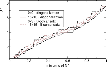
Figure 2: Eigenvalues $\lambda_{n}$, arranged in ascending order, for the networks of size $N=9$ (black) and $N=15$ (grey) obtained for the finite network, solid lines, and from the Bloch solutions with PBC, dashed lines.

Figure 2 shows the eigenvalue spectra for two networks with sizes $N=9$ and $N=15$ each. Displayed are the results for the finite networks obtained by numerical diagonalization and for the PBC cases from the Bloch solutions. The numerical results for PBC agree exactly with the Bloch solutions within the precision of our calculations and would be indistinguishable from each other in Fig.2, therefore we display only the former. We note that the numerically determined spectra are also bound by $0$ and by $8$, although the value $8$ is only approached in the limit $N\to\infty$.

Figure 3 displays the findings for a larger network, $N=60$, again comparing the spectra of the finite network with those obtained from Eq.(13). We again note that the spectra get to be very close (a fact which was to be expected because now $N$ is larger than in Fig.2), but that the PBC case still lies systematically higher. To highlight this fact, we plotted in the inset of Fig.3 for each $n$ the difference in the values between the $\lambda_{n}$ obtained with and without PBC.

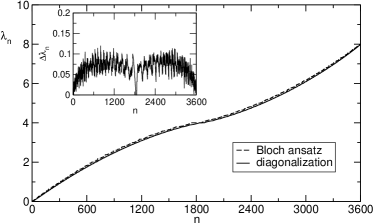
Figure 3: Eigenvalues $\lambda_{n}$, arranged in ascending order, for the network of size $N=60$. The numerical result for the finite network, solid line, is compared to the Bloch solution with PBC, dashed line. The inset shows the difference between these two results as a function of $n$.

III.2 Special initial conditions

We now turn to the dynamics of the propagation through the network and focus on special initial points. In doing so, we continue to compare our results for the finite network to the Bloch solutions. The computations for the finite network without PBC are performed by calculating all eigenvalues $\lambda_{n}$ and all eigenvectors of the matrix $\bf A$ using the FORTRAN EISPACK routine. The Bloch solutions are obtained by using the standard software packages MAPLE 7.

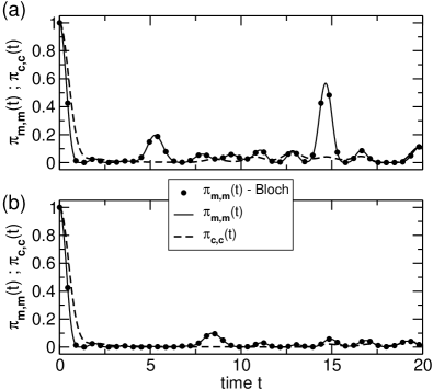
Figure 4: Probabilities for a CTQW to be at the initial site at time $t$ on networks of size (a) $N=9$ and (b) $N=15$. The starting sites are the middle node $\boldsymbol{m}$ (solid lines) and the corner node $\boldsymbol{c}$ (dashed lines), respectively. The results for the finite network, obtained by using Eq.(7), solid and dashed lines, are compared to the Bloch solutions with PBC, obtained via Eq.(14), dots, see text for details. Time is given in units of the inverse transmission rate $\gamma^{-1}$.

We begin by choosing the middle node $\boldsymbol{m}$ of the network as the starting site. Figure 4 shows the probability of being at $\boldsymbol{m}$ after time $t$ obtained via Eq.(7) for two network sizes, $N=9$ and $N=15$, respectively. Moreover, we have also inserted into Fig.4 the results obtained by starting at a corner node $\boldsymbol{c}$. Clearly, on short time scales our numerical results for $\pi_{\boldsymbol{m,m}}(t)$, solid line, agree nicely with the Bloch solutions, dots, given in Eq.(14), even for the $N=9$ network. However, the probability $\pi_{\boldsymbol{cc}}(t)$ of being at the initial corner node $\boldsymbol{c}$ after time $t$, dashed line, differs quite early from the Bloch solution, given that now the boundaries play an important role.

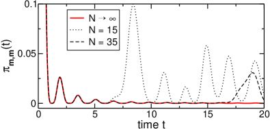
Figure 5: Comparison of the probabilities $\pi_{\boldsymbol{m,m}}(t)$ for network sizes $N=15$ and $N=35$ with the bulk system where $N\to\infty$. Time is given in units of $\gamma^{-1}$.

In order to show for finite networks the deviations from the Bloch solutions, we plot in Fig.5, for networks of sizes $N=15$ and $N=35$, the probabilities $\pi_{\boldsymbol{m,m}}(t)$ to be at time $t$ at the middle node $\boldsymbol{m}$, while also starting at $\boldsymbol{m}$. On short time scales, the $\pi_{\boldsymbol{m,m}}(t)$ behave exactly as the Bloch solution for the bulk system given in Eq.(16). However, for finite networks at longer times there is constructive interference due to the reflections at the boundaries, which result in a higher probability to find the walker back at $\boldsymbol{m}$. This interference, of course, can only take place after the wave has crossed the whole network and returns to $\boldsymbol{m}$. For the two examples given in Fig.5, this happens approximately at the times $\gamma t\approx 6.1$ for $N=15$ and $\gamma t\approx 15.6$ for $N=35$. As for the one dimensional case studied in Mülken and Blumen (2005b), such deviations are found in general at times around $N/2$.

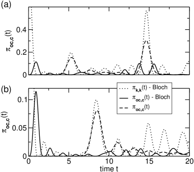
Figure 6: Probabilities for a CTQW starting at one corner node $\boldsymbol{c}$ to be at the opposite corner node $\boldsymbol{oc}$ at time $t$ on networks of size (a) $N=9$ and (b) $N=15$. The results for the finite network, obtained by using Eq.(7), dashed lines, are compared to the Bloch solutions with PBC, obtained via Eq.(14), black solid lines. We further compare also to the Bloch solution with PBC, dotted lines, where the initial and final node is the node $\boldsymbol{k}$, see Fig.4 and text for details. Time is given in units of the inverse transmission rate $\gamma^{-1}$.

In Fig.6 we show the transition probabilities $\pi_{\boldsymbol{oc,c}}(t)$ to go from one corner node $\boldsymbol{c}$ to the opposite corner node $\boldsymbol{oc}$ in time $t$. Again we take $N=9$ and $N=15$ as network sizes. We remark that already after a short period of time there is a considerable probability for the CTQW to be at the opposite node. For example, for the $N=9$ network we find that $\pi_{\boldsymbol{oc},\boldsymbol{c}}(t)\approx 0.16$ at $\gamma t\approx 5.4$. This means that for $\gamma t\approx 5.4$ a remaining probability of $0.84$ is distributed among the other $80$ nodes, which is roughly an order of magnitude less than $0.16$.

Not only is there a very high probability to go to the opposite node, but also is the transport to this node very fast. The same holds for the $N=15$ network. Here, the first peak of $\pi_{\boldsymbol{oc},\boldsymbol{c}}(t)$ occurs at about $\gamma t\approx 8.4$, for which $\pi_{\boldsymbol{oc},\boldsymbol{c}}(t)\approx 0.08$, which is again a relatively high value. We also remark that the shortest “chemical” distance between two opposite corner nodes on this network is $\Delta x=28$ bonds. Therefore, the (initial) “velocity” of the CTQW is $\Delta x/\gamma t\approx 3.3$.

For a closer examination, we also confront our calculations to the Bloch solution, see Fig.6. The results from the Bloch ansatz naturally compare only to ours where the middle node is the initial node. However, we note that the maxima of the probability $\pi_{\boldsymbol{oc,c}}(t)$ on the finite networks without PBC from a corner $\boldsymbol{c}$ to the opposite corner $\boldsymbol{oc}$ occur at approximately the same positions as the ones for $\pi_{\boldsymbol{k,k}}(t)$ from the Bloch solution for CTQWs with PBC from any node $\boldsymbol{k}$ to the same node in the same time $t$. This is quite remarkable because the distances traveled by the CTQWs are different in both cases. For the finite network of size $N=15$ without PBC, there are $28$ bonds from $\boldsymbol{c}$ to $\boldsymbol{oc}$, whereas for a network with PBC there are always $15$ bonds from $\boldsymbol{k}$ to a nearest site corresponding to the same $\boldsymbol{k}$; for the $N=9$ network, the corresponding distances are $16$ bonds and $9$ bonds, respectively. This implies that in this particular situation the initial “velocity” for the finite network is higher than the one for the network with PBC.

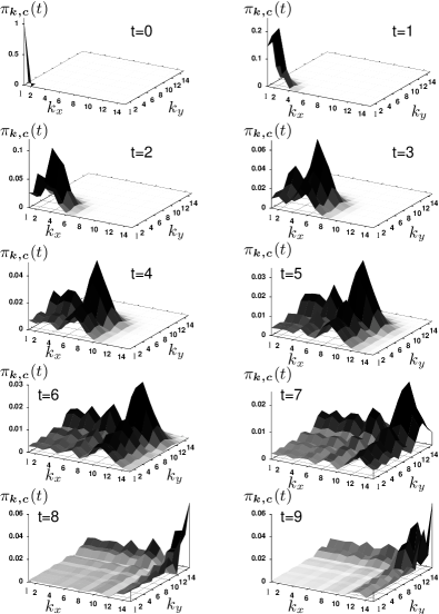
Figure 7: Snapshots of the probabilities $\pi_{\boldsymbol{k,c}}$ to be at time $t$ at node $\boldsymbol{k}$ when starting at node $\boldsymbol{c}=(1,1)$. Here the network is of size $N=15$ and time is given in units of $\gamma^{-1}$.

In Fig.7 we display snapshots in time of the transition probabilities $\pi_{\boldsymbol{k},\boldsymbol{c}}(t)$ to go from the corner node $\boldsymbol{c}=(1,1)$ to the other nodes. We see again that on short time scales the transport is very fast and, furthermore, that the main fraction of the probability stays on the diagonal. One might think that the effect is ballistic, but this is not the case: neighboring sites along the diagonal are not directly related via $\bf A$ (one may also remember that in $\bf A$ only the topology matters). The observed effect is quantum mechanical in nature: on the diagonal sites constructive interferences are particularly manifest.

The phenomenon of fast CTQW transport through the network can also be observed when starting at any other node, where on short time scales we find a high probability of going to the “mirror” node. We define the “mirror” node of $(j_{x},j_{y})$ to be $(N+1-j_{x},N+1-j_{y})$, so that the two nodes are related by inversion with respect to the center of the network.

This selective behavior has to be contrasted with the one displayed by classical CTRWs. These describe namely simple diffusion, in which no exceptional transition probabilities between particular nodes occurs.

III.3 Limiting probabilities

We continue by examining the situation at even longer times and focus in particular on the LPs $\chi_{\boldsymbol{k,j}}$ given by Eq.(8). Here, because we had already determined all eigenvalues and eigenvectors, we took advantage of the structure of Eq.(8). From Eqs.(4) and (8), and denoting the orthonormalized eigenstates of the Hamiltonian by $|\boldsymbol{q}_{n}\rangle$, such that $\sum_{n}|\boldsymbol{q}_{n}\rangle\langle\boldsymbol{q}_{n}|=\boldsymbol{1}$, we find that

$$\chi_{\boldsymbol{k,j}} =\lim_{T\to\infty}\frac{1}{T}\int\limits_{0}^{T}dt\ \left|\sum_{n}\langle\boldsymbol{k}|e^{-i{\bf H}t}|\boldsymbol{q}_{n}\rangle\langle\boldsymbol{q}_{n}|\boldsymbol{j}\rangle\right|^{2}$$

$$=\lim_{T\to\infty}\frac{1}{T}\int\limits_{0}^{T}dt\ \left|\sum_{n}e^{-i\gamma\lambda_{n}t}\langle\boldsymbol{k}|\boldsymbol{q}_{n}\rangle\langle\boldsymbol{q}_{n}|\boldsymbol{j}\rangle\right|^{2}$$

$$=\sum_{n,m}\langle\boldsymbol{k}|\boldsymbol{q}_{n}\rangle\langle\boldsymbol{q}_{n}|\boldsymbol{j}\rangle\langle\boldsymbol{j}|\boldsymbol{q}_{m}\rangle\langle\boldsymbol{q}_{m}|\boldsymbol{k}\rangle$$

$$\times\left(\lim_{T\to\infty}\frac{1}{T}\int\limits_{0}^{T}dt\ e^{-i(\lambda_{n}-\lambda_{m})\gamma t}\right)$$ (17a)

$$=\sum_{n,m}\delta_{\lambda_{n},\lambda_{m}}\langle\boldsymbol{k}|\boldsymbol{q}_{n}\rangle\langle\boldsymbol{q}_{n}|\boldsymbol{j}\rangle\langle\boldsymbol{j}|\boldsymbol{q}_{m}\rangle\langle\boldsymbol{q}_{m}|\boldsymbol{k}\rangle.$$ (17b)

We note that the integral in Eq.(17a) equals $1$ if $\lambda_{n}=\lambda_{m}$ and $0$ otherwise, i.e., it equals $\delta_{\lambda_{n},\lambda_{m}}$. Given that some eigenvalues of $\bf H$ are degenerate, the sum in Eq.(17b) can contain terms belonging to different eigenstates $|\boldsymbol{q}_{n}\rangle$ and $|\boldsymbol{q}_{m}\rangle$. Equation (17b) provides a numerically very efficient way of computing the $\chi_{\boldsymbol{k,j}}$. Remarkably, we find that the $\chi_{\boldsymbol{k,j}}$ depend in an unexpected way on the exact value of the size $N$ of the finite network under study. Given these unexpected findings, which we report in the following, we cross-checked our evaluation method based on Eq.(17b) very carefully, by comparing it in selected cases to the direct evaluation of the integral in Eq.(8). In so doing, we fixed the upper integration limit to a very large value and verified that even larger values didn’t lead to any changes in $\chi_{\boldsymbol{k,j}}$. In all cases we found that both numerical methods agree to very high precision. Thus, in general we prefered to work with Eq.(17b), which is computationally much faster than Eq.(8).

In Fig.8 we present $\chi_{\boldsymbol{k,m}}$ for CTQWs, in which the starting node is the middle node $\boldsymbol{m}$. We display results for networks of sizes $N=9$ and $N=15$. Note that the $\chi_{\boldsymbol{k,m}}$ are symmetric about the initial middle node $\boldsymbol{m}$, meaning that a node and its “mirror” node have the same limiting probabilities. This is in no way surprising, because this symmetry is already inherent in $\bf A$ and $\bf H$. More remarkable are the patterns obtained. They may be contrasted to the classical CTRW, in which the limiting probability distribution is uniform, thus symmetric for all nodes.

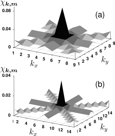
Figure 8: Limiting probabilities $\chi_{\boldsymbol{k,m}}$ to be at node $\boldsymbol{k}$ when starting at the middle node $\boldsymbol{m}$ for networks of sizes (a) $N=9$ and (b) $N=15$. The results are obtained from Eq.(17b).

Also when starting at a corner node $\boldsymbol{c}$, we often find that the LPs for the starting node and its “mirror” node are equal. In Fig.9 we show the $\chi_{\boldsymbol{k,c}}$ obtained by going from the corner node $\boldsymbol{c}=(1,1)$ to the other nodes for networks of sizes $N=5$, $N=14$, $N=23$, and $N=47$.

However, for some particular network sizes the distributions of the LPs turn out to be asymmetric. For instance, for a network of size $N=15$ the LP $\chi_{\boldsymbol{oc,c}}$ for the CTQW starting at node $\boldsymbol{c}$ to be at the opposite corner node $\boldsymbol{oc}$ is less than the LP $\chi_{\boldsymbol{c,c}}$ to be at the initial node. The same is true for the nodes along the edges of the network. Figure 10 shows that such asymmetries occur for networks of the sizes $N=6$, $N=15$, $N=24$, and $N=48$ (the asymmetries are best seen by looking at $\chi_{\boldsymbol{c,c}}$ and $\chi_{\boldsymbol{oc,c}}$). Note that these asymmetries occur for networks in which $N$ is increased only by unity compared to networks which behave symmetrically, e.g., see Fig.9. The smallest network where we detected asymmetries in the distribution of the LPs has $N=6$. The next ones we found for $N=12,15,18,21,24,30,36,\cdots$.

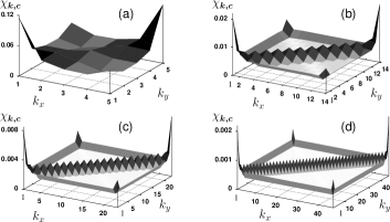
Figure 9: As in Fig.8, LPs $\chi_{\boldsymbol{k,c}}$ to be at node $\boldsymbol{k}$ when starting at the corner node $\boldsymbol{c}=(1,1)$ for networks of sizes (a) $N=5$, (b) $N=14$, (c) $N=23$, and (d) $N=47$.

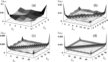
Figure 10: As in Fig.8, LPs $\chi_{\boldsymbol{k,c}}$ to be at node $\boldsymbol{k}$ when starting at the corner node $\boldsymbol{c}=(1,1)$ for networks of sizes (a) $N=6$, (b) $N=15$, (c) $N=24$, and (d) $N=48$. One may note the asymmetries by comparing to Fig.9.

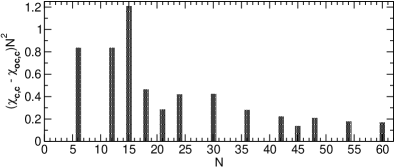
Figure 11: Differences between the LPs for CTQWs that start at $\boldsymbol{c}=(1,1)$ to be at $\boldsymbol{c}$, $\chi_{\boldsymbol{c},\boldsymbol{c}}$, or to be at its “mirror” node $\boldsymbol{oc}=(N,N)$, $\chi_{\boldsymbol{oc},\boldsymbol{c}}$, as a function of the network size $N$, for $1\leq N\leq 60$.

The asymmetries are small and therefore not easy to spot in the global pictures displayed in Figs.9 and 10. As illustrative examples, we choose prominent points in the network to show the asymmetries. An asymmetric LP distribution is particularly evident in the difference between $\chi_{\boldsymbol{c,c}}$ and $\chi_{\boldsymbol{oc,c}}$. Thus, as an overview we present in Fig.11 as a function of $N$ a plot of the $(\chi_{\boldsymbol{c,c}}-\chi_{\boldsymbol{oc,c}})N^{2}$ values obtained. Note that all $N$ values in Fig.11 for which $(\chi_{\boldsymbol{c,c}}-\chi_{\boldsymbol{oc,c}})\neq 0$ are divisible by $3$. However, the converse is not true, we find symmetric LP distributions for the networks with $N=3,9,27,33,39,\cdots$. The general $N$-dependence of $\chi_{\boldsymbol{oc,c}}(N)$ and $\chi_{\boldsymbol{m,m}}(N)$ is plotted in Fig.12. In contrast to the classical limiting probability, which in all cases shows equipartition between all nodes, i.e. it is given by $N^{-2}$, we find that $\chi_{\boldsymbol{oc,c}}(N)$ and $\chi_{\boldsymbol{m,m}}(N)$ decay nearly algebraically, namely as $N^{-3/2}$.

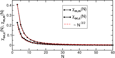
Figure 12: $N$-dependence of the LPs $\chi_{\boldsymbol{oc,c}}(N)$ and $\chi_{\boldsymbol{m,m}}(N)$. For $\chi_{\boldsymbol{m,m}}(N)$ only odd numbered networks are shown, since only those have a single central node $\boldsymbol{m}$.

Another striking feature of the CTQW is that the LPs display quite regular patterns over the network. For the CTQW starting at the network’s middle node $\boldsymbol{m}$, the distributions of the LPs show a star-like pattern, see Fig.8. In all cases studied here, the LP distribution is such that its major fraction appears to be distributed along lines diagonal and parallel to the network’s edges and crossing each other at the initial node. Here again this implies that the transport is generated by constructive and destructive interference. This might have consequences: On a regular, square network (or on a lattice for that matter) the application of the CTQW as a search algorithm is flawed, since its effectiveness is correlated with the initial site. That is, there is a high probability of finding a certain node which is “constructively” correlated with the initial one, but there is also a rather low probability of finding the others. Thus, although the topology of the square network has no exceptional sites, the transport through the lattice strongly depends on the initial condition. This relates directly to previous studies, where it was found that quantum transport can become much slower than the classical one Mülken and Blumen (2005a). However, there it was also shown that if one starts in a superposition of states, the transport can get to be much quicker than in the classical case. A similar effect should also be observable here. For instance, if one starts in a uniform superposition of states along the baseline of the network, the CTQW can be mapped onto a one dimensional problem, as treated for instance in Childs et al. (2002).

Furthermore, the fact that the LP distributions have especially high peaks at the initial node and at its “mirror” node strongly recalls (in the spatially discrete version discussed here) the quantum mirage effects found in elliptic quantum corrals; these, again, can be related to wave interferences, see for instance Manoharan et al. (2000); Fiete and Heller (2003). A more detailed study of this effect will be published elsewhere Mülken et al. (2005).

IV Conclusion

We have studied numerically continuous-time quantum walks on finite networks topologically equivalent to square lattices. Furthermore, we compared our results to analytic expressions obtained from the Bloch ansatz for networks with periodic boundary conditions. For these quantum walks, we have found that on short time scales a directed transport through the network takes place. In particular, when placing the initial excitation at one corner node, the walks propagate in a rather direct fashion along the diagonal to the opposite corner node. The transport is not ballistic, but is rather due to constructive quantum mechanical interferences.

In the long time limit, we found that walks on networks of specific sizes $N$ may show (in a totally unexpected way) asymmetric limiting probability distributions. This asymmetry manifests itself in the fact that the limiting probabilities for a CTQW to be at the initial node $\boldsymbol{c}=(1,1)$ and at its “mirror” node $\boldsymbol{oc}=(N,N)$ differ. However, we were unable to find a way to predict which particular $N$ values are related to such asymmetries.

In general, the limiting probability distributions show patterns which depend on the starting site of the CTQW. This is a remarkable effect, which might have consequences for search algorithms based on CTQWs. Furthermore, we also found in all our calculations that the limiting probability distributions show strong peaks at the initial node and its “mirror” node. This effect resembles a discrete version of quantum mirages.

References

- Nielsen and Chuang (2000) M. A. Nielsen and I. L. Chuang, Quantum Computation and Quantum Information (Cambridge University Press, Cambridge, England, 2000).
- Childs and Goldstone (2004) A. M. Childs and J. Goldstone, Phys. Rev. A 70, 022314 (2004).
- Shenvi et al. (2003) N. Shenvi, J. Kempe, and K. B. Whaley, Phys. Rev. A 67, 052307 (2003).
- Aharonov et al. (1993) Y. Aharonov, L. Davidovich, and N. Zagury, Phys. Rev. A 48, 1687 (1993).
- Farhi and Gutmann (1998) E. Farhi and S. Gutmann, Phys. Rev. A 58, 915 (1998).
- Kempe (2003) J. Kempe, Contemporary Physics 44, 307 (2003).
- Childs et al. (2002) A. M. Childs, E. Farhi, and S. Gutmann, Quantum Information Processing 1, 35 (2002).
- Mülken and Blumen (2005a) O. Mülken and A. Blumen, Phys. Rev. E 71, 016101 (2005a).
- Wójcik and Dorfman (2002) D. K. Wójcik and J. R. Dorfman, Phys. Rev. E 66, 036110 (2002).
- Wójcik and Dorfman (2003) D. K. Wójcik and J. R. Dorfman, Phys. Rev. Lett. 90, 230602 (2003).
- Mülken and Blumen (2005b) O. Mülken and A. Blumen, Phys. Rev. E 71, 036128 (2005b).
- Ziman (1972) J. M. Ziman, Principles of the Theory of Solids (Cambridge University Press, Cambridge, England, 1972).
- Kittel (1986) C. Kittel, Introduction to Solid State Physics (Wiley, New York, 1986).
- Weiss (1994) G. H. Weiss, Aspects and Applications of the Random Walk (North-Holland, Amsterdam, 1994).
- van Kampen (1990) N. van Kampen, Stochastic Processes in Physics and Chemistry (North-Holland, Amsterdam, 1990).
- Aharonov et al. (2001) D. Aharonov, A. Ambainis, J. Kempe, and U. Vazirani, in Proceedings of ACM Symposium on Theory of Computation (STOC’01) (ACM Press, New York, 2001), p. 50.
- Gurtovenko and Blumen (2002) A. A. Gurtovenko and A. Blumen, Macromolecules 35, 3288 (2002).
- Blumen and Merkel (1977) A. Blumen and C. Merkel, Phys. Status Solidi B 83, 425 (1977).
- Streitwieser (1961) A. Streitwieser, Molecular Orbital Theory (Wiley, New York, 1961).
- McQuarrie (1983) D. A. McQuarrie, Quantum Chemistry (Oxford University Press, Oxford, 1983).
- Ito (1987) K. Ito, ed., Encyclopedic Dictionary of Mathematics (MIT-Press, Cambridge, MA, 1987).
- Tregenna et al. (2003) B. Tregenna, W. Flanagan, R. Maile, and V. Kendon, New J. Phys. 5, 83 (2003).
- Travaglione and Milburn (2002) B. C. Travaglione and G. J. Milburn, Phys. Rev. A 65, 032310 (2002).
- Ahmadi et al. (2002) A. Ahmadi, R. Belk, C. Tamon, and C. Wendler, arXiv: quant-ph/0209106 (2002).
- Adamczak et al. (2003) W. Adamczak, K. Andrew, P. Hernberg, and C. Tamon, arXiv: quant-ph/0308073 (2003).
- Smith et al. (1976) B. T. Smith, J. M. Boyle, B. S. Garbow, Y. Ikebe, V. C. Klema, and C. B. Moler, Matrix eigensystem routines - EISPACK Guide, vol. 6 of Lecture notes in computer science (Springer, Berlin, 1976).
- Manoharan et al. (2000) H. C. Manoharan, C. P. Lutz, and D. M. Eigler, Nature 403, 512 (2000).
- Fiete and Heller (2003) G. A. Fiete and E. J. Heller, Rev. Mod. Phys. 75, 933 (2003).
- Mülken et al. (2005) O. Mülken, A. Volta, and A. Blumen, in preparation (2005).