Anomalies of Wave-Particle Duality due to Translational-Internal Entanglement

Abstract

We predict that if internal and momentum states of an interfering object are correlated (entangled), then by measuring its internal state we may infer both path (corpuscular) and phase (wavelike) information with much higher precision than for objects lacking such entanglement. We thereby partly circumvent the standard complementarity constraints of which-path detection.

Our ability to know the actual path taken by a diffracting or interfering particle has been debated since the early days of quantum mechanics: suffice it to recall the Bohr–Einstein “which-path” controversy in the context of two–slit interference Zurek . More recent analysis of this issue has prompted the formulation Wooters ; ScullyNature and subsequent testing RempeNature ; Mei of the fundamental complementarity relation $D^{2}+V^{2}\leq 1$ between path distinguishability $D$, which is the certitude of knowing the actual path of an interfering particle by coupling a detector to one of these paths, and the fringe visibility (contrast) $V$, which determines the ability to infer the phase difference between the alternative paths. But must “which-path” information always come at the expense of interference-phase information? We show that this is not necessarily the case when internal and momentum states of the interfering particle become entangled. Then, by measuring its internal state we may infer both path (corpuscular) and phase (wavelike) information with much higher precision than for objects lacking such entanglement, thereby partly circumventing the complementarity constraints. This anomaly may yield novel interferometric applications.

Consider spin-1/2 particles (or their analogs: two-level atoms) of mass $M$ that are prepared in the four–dimensional (4D) input state

$$|\psi_{\mathrm{input}}\rangle=\left(\sqrt{1-p}|k_{1}\rangle|1\rangle+\sqrt{p}|k_{2}\rangle|2\rangle\right).$$ (1)

Here $\sqrt{1-p}$ and $\sqrt{p}$ are the probability amplitudes (chosen to be real and positive) of the internal states $|1\rangle,|2\rangle$, which correspond to the internal energy levels $\epsilon_{1},\epsilon_{2}$. These states are assumed to have $x$-oriented momenta, $\hbar k_{1},\hbar k_{2}$, constrained by the total energy of state (1):

$$E=\frac{\hbar^{2}k_{1}^{2}}{2M}+\epsilon_{1}=\frac{\hbar^{2}k_{2}^{2}}{2M}+\epsilon_{2}.$$ (2)

The choice (2) enforces a stationary (time-independent) scenario in what follows. We use Eq.(1) as a short-hand description of narrow-momentum wavepackets (gaussians) whose coherence length along $x$ exceeds the size of the interferometric setup $L$. This implies that $|k_{1(2)},1(2)\rangle$ really represent $\int dkf_{1(2)}(k)|k,1(2)\rangle$, with gaussian distributions $f_{1(2)}(k)\propto\exp(-|k-k_{1(2)}|^{2}/\Delta_{x}^{2})$, such that $\Delta_{x}\ll 1/L$.

We are interested in the peculiar spatial properties of the stationary state (1), which exhibits a feature that has hitherto not been studied in the context of single-particle interferometry: Bell-like Scully quantum correlation between two momentum states and two nondegenerate internal states, hereafter named translational-internal entanglement (TIE). This entanglement vanishes for $p=0,1$ and is maximal for $p=1/2$. The realization of TIE is discussed later on.

We will show that the TIE state (1) yields much more information than unentangled states on propagation along both arms of the simple Mach-Zehnder interferometer Scully (MZI). The wavefunction $\langle x|\psi_{\mathrm{input}}\rangle=\left(\sqrt{1-p}e^{ik_{1}x}|1\rangle+\sqrt{p}e^{ik_{2}x}|2\rangle\right)$ is “split” at the balanced (50%-50%) input beam splitter (BS1) into two beams that propagate along either of the two arms of length $L_{A}$ or $L_{B}$, then recombine at the 50%-50% beam merger BS2 (Fig. 1a). Propagating these beams along the two arms, we find that right before the beam merger the “final” wavefunction is, in the $x$ representation

$$|\psi_{f}\rangle_{x} = \frac{1}{\sqrt{2}}\left(|\psi_{Af}\rangle_{x}|A\rangle+|\psi_{Bf}\rangle_{x}|B\rangle\right),$$ (3)

$$|\psi_{Af}\rangle_{x} \equiv \langle x|\psi_{Af}\rangle=\left(\sqrt{1-p}e^{i\phi_{A1}}|1\rangle_{A}+\sqrt{p}e^{i\phi_{A2}}|2\rangle_{A}\right),$$

$$|\psi_{Bf}\rangle_{x} \equiv \langle x|\psi_{Bf}\rangle=\left(\sqrt{1-p}e^{i\phi_{B1}}|1\rangle_{B}+\sqrt{p}e^{i\phi_{B2}}|2\rangle_{B}\right).$$

In (3), we have introduced $|A\rangle$ and $|B\rangle$, the spatially–orthogonal states representing the respective paths (which means that the spatial width of the wave packet perpendicular to the propagation ($x$-) axis is much smaller than the distance between arms A and B). We have also introduced in (LABEL:e3) the phases $\phi_{A1(2)}=k_{1(2)}L_{A}$, $\phi_{B1(2)}=k_{1(2)}L_{B}$. As $k_{1(2)}L_{A},k_{1(2)}L_{B}\rightarrow 2m\pi$, we recover from (LABEL:e3) the input states in arms A,B. We see that a single-arm contribution to the wavefunction, $|\psi_{Af}\rangle$ or $|\psi_{Bf}\rangle$, is rotated by the phase $\phi_{A2}-\phi_{A1}=(k_{2}-k_{1})L_{A}$ or $\phi_{B2}-\phi_{B1}=(k_{2}-k_{1})L_{B}$, respectively. These phases, representing the interference of $|k_{1}\rangle|1\rangle$ and $|k_{2}\rangle|2\rangle$, distinguish TIE from standard states: they are “which-path” markers travelling with the particle, encoding the path traversed along each arm in the superposition of internal states $|1\rangle$ and $|2\rangle$, as in a Ramsey interferometer Scully .

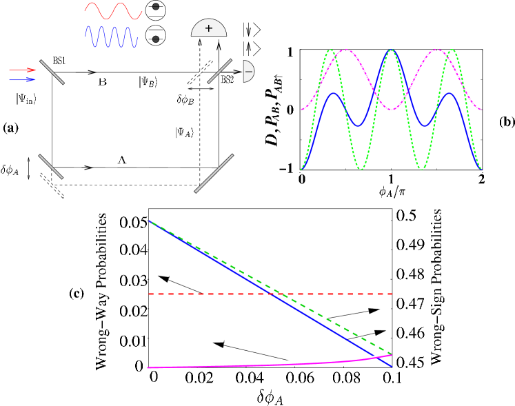
Figure 1: (a) A particle in the TIE state (1) in a MZI. It traverses the interferometer from BS1 to BS2 via paths A and B, whose mean phases, $\phi_{A1(2)}=k_{1(2)}L_{A}$ and $\phi_{B1(2)}=k_{1(2)}L_{B}$, fluctuate by $(\delta\phi_{A})_{1(2)}$ and $(\delta\phi_{B})_{1(2)}$, respectively. Both output detectors $+$ and $-$ discriminate internal states $|\uparrow\rangle$ and $|\downarrow\rangle$ (eq. (7)). (b) The $\phi_{A1}$ dependence of TIE functions. (eqs. (8), (10)) for $p=1/2,k_{2}=3k_{1}$, $\phi_{B1}=\pi$: non-sinusoidal $P_{AB\uparrow}$ (solid-bold-blue), $D_{\rm TIE}$ (dash-dot,magenta); sinusoidal $P_{AB}$ (dashed,green, $V=1$) for $3k_{1}=3k_{2}=k_{\rm max}$ (standard case). (c) Wrong-way and wrong-phase probabilities for TIE (solid magenta and solid blue, respectively - Eq. (10)) are lower than for the standard case (dashed red and dashed green, respectively - Eq. (13) for $D_{S}=0.95$) as functions of $|\delta\phi_{A}|$.

This feature of TIE allows us to record the interference of four distinct contributions of paths A and B (rather than the usual two). It will be shown that by reading out this interference at the output detectors, we may infer, with much higher certitude than for standard states, parameters whose knowledge is usually complementary: the path (arm) state ($|A\rangle$ or $|B\rangle$) and the phase (length) difference of the two interfering arms. At the output detectors $+$ and $-$ (Fig. 1a), the wavefunctions are, respectively, the sum and the difference of the $A$ and $B$ path amplitudes Scully

$$|\psi_{\pm}\rangle = \frac{1}{2}\left(|\psi_{Af}\rangle_{x}\pm|\psi_{Bf}\rangle_{x}\right)|\pm\rangle$$ (5)

$$= \frac{1}{2}\left[\sqrt{1-p}\left(e^{i\phi_{A1}}\pm e^{i\phi_{B1}}\right)|1\rangle\right.$$

$$+ \left.\sqrt{p}\left(e^{i\phi_{A2}}\pm e^{i\phi_{B2}}\right)|2\rangle\right]|\pm\rangle.$$

We henceforth choose, for the sake of concreteness, $k_{2}=3k_{1}$, denoting $\phi_{A1}-\phi_{B1}\equiv\phi,\phi_{A2}-\phi_{B2}=3\phi$. If we now ignore the internal states of the particle, we get the following click probabilities at the +/$-$ detectors,

$$P_{\pm}=\langle\psi_{\pm}|\psi_{\pm}\rangle\equiv\frac{1}{2}\left[1\pm(1-p)\cos\phi\pm p\cos 3\phi\right].$$ (6)

This procedure yields no which-path (arm) information, only phase-difference information.

In order to gain both path and phase information, our output detectors +/$-$ should discriminate between internal states, such that each detector projects onto one of the orthogonal states

$$|\uparrow\rangle = \frac{1}{\sqrt{2}}\left(|1\rangle+|2\rangle\right),$$

$$|\downarrow\rangle = \frac{1}{\sqrt{2}}\left(|1\rangle-|2\rangle\right).$$ (7)

This setup has four different output (detection) channels: $+\uparrow,+\downarrow,-\uparrow,-\downarrow$. The $+\uparrow$ and $-\uparrow$ channel probabilities are obtained upon projecting the wavefunctions $|\psi_{\pm}\rangle$ onto $|\uparrow\rangle$. We shall analyze them explicitly for maximum TIE, $p=1/2$, which will be shown to be the optimal choice. These probabilities are:

$$P_{\pm\uparrow} = \frac{1}{2}\left(P_{A\uparrow}+P_{B\uparrow}\pm P_{AB\uparrow}\right),$$

$$P_{A\uparrow} = \frac{1}{4}\left[1+\cos\left(2\phi_{A}\right)\right],$$

$$P_{B\uparrow} = \frac{1}{4}\left[1+\cos\left(2\phi_{B}\right)\right],$$

$$P_{AB\uparrow} = \frac{1}{4}\left[\cos\phi+\cos 3\phi+\cos\left(3\phi_{B}-\phi_{A}\right)\right.$$ (8)

$$+ \left.\cos\left(3\phi_{A}-\phi_{B}\right)\right].$$

Here $P_{A\uparrow}$ denotes the joint probability of finding the particle right before BS2 in arm A in the internal state $\uparrow$, and similarly for $P_{B\uparrow}$. The $P_{AB\uparrow}$ term is the interference contribution to the $\uparrow$ channel. The $\downarrow$ channel probabilities are obtained from (8) upon replacing + by $-$ in front of all cosine terms except for cos $\phi$ and cos $3\phi$.

Equation (8) implies that, due to TIE, the single-arm contributions $P_{A\uparrow}$ and $P_{B\uparrow}$ (or their $\downarrow$ counterparts) have sinusoidal dependence on the phases, as compared to the non-sinusoidal, complicated phase dependence of the arm-interference contribution $P_{AB\uparrow}$ (see Fig. 1b). This difference in phase dependence will be shown to be crucial for inferring the path (arm) together with the small phase deviations (path-length deviations) $\pm\delta\phi_{A(B)}$ around their mean values $\overline{\phi_{A(B)}}\equiv k_{1}\overline{L}_{A(B)}$.

If $N_{\rm in}$ particles travel through the MZI, then we obtain from (8) the “imbalance” $(\delta N)_{\uparrow}$ between the counts of the two output detectors and the total number $(N_{\rm tot})_{\uparrow}$ counts at both detectors in the $\uparrow$ channel. As an example we choose $\overline{\phi_{A(B)}}$ such that $P_{B\uparrow}\approx 1/2$, $P_{A\uparrow}\approx 0$: $\overline{\phi}_{B}=\pi$, $\overline{\phi}_{A}=\frac{\pi}{2}$, and consider small length deviations $\delta\phi_{A}\equiv k_{1}\delta L_{A}$, $\delta\phi_{B}\equiv k_{1}\delta L_{B}$. Then

$$(N_{+})_{\uparrow}-(N_{-})_{\uparrow} \equiv \left(\delta N\right)_{\uparrow}=N_{\rm in}\left(P_{+\uparrow}-P_{-\uparrow}\right)$$

$$= N_{\rm in}P_{AB\uparrow}\approx-N_{\rm in}\delta\phi_{A},$$

$$(N_{+})_{\uparrow}+(N_{-})_{\uparrow} \equiv \left(N_{\rm tot}\right)_{\uparrow}=N_{\rm in}(P_{A\uparrow}+P_{B\uparrow})$$ (9)

$$\approx \frac{N_{\rm in}}{2}\left(1-\delta\phi_{B}^{2}+\delta\phi_{A}^{2}\right).$$

Hence, upon varying $\delta\phi_{A}=k_{1}\delta L_{A}$, we may deduce that $(N_{\rm tot})_{\uparrow}$ has a contribution from the unlikely path $N_{\rm in}P_{A\uparrow}$, which scales quadratically with $\delta\phi_{A}$, whereas $(\delta N)_{\uparrow}$, which is proportional to the path-interference probability $(P_{AB})_{\uparrow}$ of $|\uparrow\rangle$ particles, depends linearly on $\delta\phi_{A}$. The same conclusions apply to the $\downarrow$ channels upon exchanging A and B, whereupon $P_{A\downarrow}\approx 1/2-\delta\phi_{A}^{2}/2$, $P_{B\downarrow}\approx\delta\phi_{B}^{2}/2$, $P_{AB\downarrow}\approx\delta\phi_{B}$. Thus, we conclude that the particle has most likely traversed path A if it is found in state $|\downarrow\rangle$ or path B if it is found in $|\uparrow\rangle$.

The information on the likelihood of traversing paths A, B or both, embodied by Eqs.(8), (Anomalies of Wave-Particle Duality due to Translational-Internal Entanglement), is inferred without which-path detection inside the MZI. But is the concept of likely (“correct”) or unlikely (“wrong”) paths meaningful at all here? As we will detail elsewhere, this concept is meaningful, since we may verify our inferences for small subensembles, and compare the errors of these inferences to those obtainable in the standard case by conventional which-path detection. The probabilities of our wrong-way and wrong-phase guesses per particle are expected from (8), (Anomalies of Wave-Particle Duality due to Translational-Internal Entanglement) to be (see Fig. 1c)

$$\left(P_{\stackrel{{\scriptstyle\rm wrong}}{{\rm way}}}\right)_{\rm TIE} = P_{A\uparrow}+P_{B\downarrow}\approx\frac{\delta\phi_{A}^{2}}{2},$$ (10)

$$\left(P_{\stackrel{{\scriptstyle\rm wrong}}{{\rm phase}}}\right)_{\rm TIE} = P_{+}(-|\delta\phi_{A}|)=P_{-}(+|\delta\phi_{A}|)$$

$$\approx \frac{1}{2}(1-|\delta\phi_{A}|).$$

To extract both path and phase information in the absence of TIE, when $k\equiv k_{1}=k_{2}$, we are forced to adopt the standard recipe Zurek ; Wooters ; ScullyNature ; RempeNature of placing a detector in one of the arms inside the MZI. Let this detector be imperfect, allowing path distinguishability $D_{S}<1$. This path distinguishability is phase-independent, i.e. it does not depend on $\phi=k(L_{A}-L_{B})$. The interference at the output detector then oscillates as

$$\left(P_{\pm}\right)_{S}=\frac{1}{2}\pm\frac{V\cos\phi}{2},$$ (11)

the visibility $V$ being complementary to the distinguishability ScullyNature :

$$V^{2}+D_{S}^{2}=1.$$ (12)

The counterparts of (10) are then the error probabilities (see Fig. 1c):

$$\left(P_{\stackrel{{\scriptstyle\rm wrong}}{{\rm way}}}\right)_{S} = \frac{1-D_{S}}{2},$$ (13)

$$\left(P_{\stackrel{{\scriptstyle\rm wrong}}{{\rm phase}}}\right)_{S} \approx \frac{1}{2}(1-\sqrt{1-D_{S}^{2}}|\delta\phi|).$$

It can be checked that the TIE-based guesses (10) permit higher statistical confidence (smaller error) of extracting both path and phase information (with equal weights), than their standard-case counterparts (13).

In order to compare the information obtainable by the TIE-based and standard strategies, it is instructive to examine the complementary quantities recently introduced Jakob for entangled two-qubit systems:

(i) The concurrence, a measure of the two-qubit entanglement, becomes for the TIE wavefunctions (5) ($k_{2}/k_{1}=3$):

$$C_{\rm TIE} \equiv |\langle(\psi_{+}+\psi_{-})|\sigma_{y}\otimes\sigma_{y}|(\psi_{+}+\psi_{-})^{*}\rangle|$$ (14)

$$= 2\sqrt{p(1-p)}|\sin{\phi}|,$$

where $\sigma_{y}$ is the appropriate Pauli matrix. If we define the analog of path distinguishability $D_{S}$ ScullyNature for TIE,
$(P_{\stackrel{{\scriptstyle\rm wrong}}{{\rm way}}})_{\rm TIE}\equiv(1-{\cal D})/2$, then, to $\delta\phi^{2}$ accuracy, $C_{\rm TIE}={\cal D}$ (cf. Eq.(10) for $p=1/2$). The peculiarity of TIE is that ${\cal D}$ is phase dependent.

(ii) The coherence, alias the generalized visibility ${\cal V}$ defined in Jakob , becomes for the TIE states (3): ${\cal V}=\sqrt{(1-p)^{2}+p^{2}+2p(1-p)\cos{2\phi}}$ ($k_{2}/k_{1}=3$). This measure oscillates with $\phi$. Hence, although, for any phase $\phi$

$${\cal D}^{2}+{\cal V}^{2}=1$$ (15)

in accordance with the known complementarity relation ScullyNature ; Jakob , ${\cal V}$ does not describe the amplitude of the TIE nonsinusoidal interference pattern (6), but rather the purity of the two-path state. We may instead invoke the customary visibility ScullyNature ; RempeNature ; Mei ; Scully $V=\max\,(P_{+}-P_{-})=\max\,(P_{AB})=1$. This global (phase-independent) measure would then yield, for phases such that ${\cal D}\simeq 1$: ${\cal D}^{2}+V^{2}\simeq 2$, at odds with standard complementarity! Yet this complementarity violation merely demonstrates the inadequacy of the customary definitions for the TIE nonsinusoidal interference pattern.

We are therefore led to conclude that the phase information stored in the TIE pattern requires a new operationally-oriented measure. An adequate measure is the phase-sensitivity, expressing the phase-derivative of $(P_{AB})_{\downarrow}$ or $(P_{AB})_{\uparrow}$ in (8) or $P_{\pm}$ in (6):

$${\cal S}\equiv\left|\frac{2{\rm d}P_{\pm}}{k_{\rm max}{\rm d}L}\right|=\frac{1}{3}|(p-1)\sin{\phi}-3p\sin{3\phi}|,$$ (16)

where we have chosen $k_{\rm max}L=3k_{1}L=3\phi$. Because we are interested in maximizing both ${\cal S}$ and ${\cal D}$, we restrict $p$ to the region $p\in(1/2,1)$ and $\phi$ to the vicinity of $\pi/2$. After eliminating $p$ from Eq.(14) we get the following ellipse equation (for the choice $k_{2}=3k_{1}$)

$$\frac{\left[{\cal S}+\frac{\sin{\phi}+3\sin{3\phi}}{6}\right]^{2}}{\frac{|\sin{\phi}-3\sin{3\phi}|^{2}}{36}}+\frac{{\cal D}^{2}}{|\sin{\phi}|^{2}}=1.$$ (17)

Extending Eq.(17) to any integer ratio $k_{2}/k_{1}=N$ we get the generalized complementarity relation for TIE (at the respective optimal phase value)

$$\frac{\left({\cal S}-\frac{N-1}{2N}\right)^{2}}{\frac{\left(N+1\right)^{2}}{4N^{2}}}+{\cal D}^{2}=1.$$ (18)

The relation (18) is our main result. When $N=1$, setting ${\cal D}=D_{S}$ and using the same definition of sensitivity as for TIE (Eq.(16)) we obtain, for the optimal phase $\phi\approx\pi/2$, the sensitivity ${\cal S}=V$ and recover the standard complementarity relation of Eq.(12).

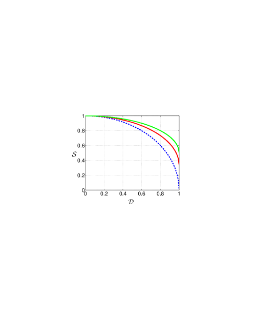
Figure 2: Comparison of the ${\cal S}$, ${\cal D}$ dependence for standard case $N=1$, Eq.(12) (dashed-blue) and the TIE cases Eq.(19) (red) and Eq.(20) (green) at the optimal phases.

The standard complementarity circle (12) ($N=1$) encloses a smaller area in the ${\cal S}$-${\cal D}$ plane than the TIE complementarity ellipse with $N>1$ (Fig.(2)). This area difference is a measure of the additional information on the paths stored in TIE patterns compared to the standard case: higher ${\cal S}$ for the same ${\cal D}$ , or vice versa. As $N$ increases, so does the area difference. The choice $N=3$ ($k_{2}=3k_{1}$) and $\phi\approx\pi/2$, discussed in Eqs.(6-10), yields

$$\frac{({\cal S}-\frac{1}{3})^{2}}{\frac{4}{9}}+{\cal D}^{2}=1.$$ (19)

For $N\gg 1$ we find the largest additional information

$$\frac{({\cal S}-\frac{1}{2})^{2}}{\frac{1}{4}}+{\cal D}^{2}=1.$$ (20)

TIE is realizable by forces changing the momentum depending on the internal state as in Stern-Gerlach setups Scully . TIE interferometry may use e.g., molecules Buzek . Here we discuss the following realizations: (i) An optical TIE setup may involve an entirely birefringent MZI. Polarization states $|1\rangle$ and $|2\rangle$ are then entangled throughout the MZI with wavevectors $k_{1}$ and $k_{2}$, so that $\phi_{A2}-\phi_{A1}$ or $\phi_{B2}-\phi_{B1}$ in (8) may attain $\pi$ if $L_{A},L_{B}$ exceed 0.1mm. (ii) An atomic realization may involve the experimentally tested RempeNature atomic MZI based on Bragg scattering of a cold ⁸⁵Rb atom from standing light waves. We may envisage a cold ⁸⁵Rb atom, moving vertically along the $z$ -axis with momentum $\hbar k_{z}$, $\hbar k_{x}=0$, its internal state being the lowest hyperfine level, $F=2$. A Ramsey RF field prepares the superposition between states $F=2$ and $F=3$. Subsequently, as the atom moves through two travelling Bragg gratings, each hyperfine state “feels” a different grating (by tuning the field of each grating close to resonance with a different electronic transition) such that the atoms in the states $F=2$ and $F=3$ are Bragg-reflected to acquire, e.g., transverse wavenumbers, $k_{1}=k_{x}$ and $k_{2}=3k_{x}$, respectively. The atom is thereby prepared in the TIE state (1), with $N=3$, which can then travel through the MZI. At the output, one can project the internal states on a suitable basis, by another Ramsey RF field.

The overlap of the wavepackets centered at $k_{1}$ and $k_{2}$ decreases as they propagate. This reduces our ability to distinguish the paths via the coherence between internal states $|1\rangle$ and $|2\rangle$, as per Eqs.(5)-(8). If either the $k_{x}$ or $3k_{x}$ wavepacket has a length $w_{1(3)}$ not much larger than the MZI length $L$, so that their overlap is incomplete at the output, the distinguishability will drop as $\exp[-AL^{2}/w_{1(3)}^{2}]$, $A$ being a constant.

The crux of our new effects is that the TIE state (1) allows us to perform unconventional “quantum erasure” Scully , providing information on both interfering paths at the expense of the internal states to which they are entangled. Standard complementarity holds for projection on one of the alternative paths $|A\rangle$ or $|B\rangle$, hampering their superposition Wooters ; ScullyNature ; RempeNature . It needs to be generalized in the present case (cf. (18)), where the 4D TIE state is projected onto an internal-state (2D) basis. We may thus acquire more information, by virtue of TIE, on any chosen 2D superposition of the $|A\rangle$ and $|B\rangle$ path states. The resulting path and phase information is real and verifiable. Such intra-particle entanglement may become a new resource of quantum information or interferometric measurements.

The support of EU (QUACS and SCALA), FRVŠ(2712/2005), GAČR(202/05/0486) and ISF is acknowledged. We thank M. Arndt, S. Dürr, B. G. Englert, G. Rempe, Y. Silberberg and A. Zeilinger for useful discussions.

References

(1) J. A. Wheeler and W. H. Zurek (ed.), Quantum Theory and
Measurement (Princeton University Press, 1983).
(2) W. K. Wootters and W. H. Zurek, Phys. Rev. D
19, 473 (1979); D. M. Greenberger and A. Yasin, Phys. Lett. A
128, 391 (1988).
(3) M.O. Scully, B.-G. Englert, H. Walther, Nature
375, 367, (1995); B.-G. Englert, Phys. Rev. Lett.
77, 2154 (1996); G.Jaeger, A. Shimony and L. Vaidman, Phys.
Rev. A 51, 54 (1995).
(4) S. Dürr, T. Nonn, and G. Rempe, Nature
395, 33 (1998).
(5) M. Mei and M. Weitz, Phys. Rev. Lett. 86,
559 (2001).
(6) M. O. Scully and M. S. Zubairy, Quantum Optics (Cambridge
University Press, 1997).
(7) M. Jakob and J. A. Bergou, quant-ph/0302075.
(8) M. Hillery, L. Mlodinow and V. Buzek, Phys. Rev. A
71, 062103 (2005).