No approximate complex fermion coherent states

Abstract

Whereas boson coherent states with complex parametrization provide an elegant, and intuitive representation, there is no counterpart for fermions using complex parametrization. However, a complex parametrization provides a valuable way to describe amplitude and phase of a coherent beam. Thus we pose the question of whether a fermionic beam can be described, even approximately, by a complex-parametrized coherent state and define, in a natural way, approximate complex-parametrized fermion coherent states. Then we identify four appealing properties of boson coherent states (eigenstate of annihilation operator, displaced vacuum state, preservation of product states under linear coupling, and factorization of correlators) and show that these approximate complex fermion coherent states fail all four criteria. The inapplicability of complex parametrization supports the use of Grassman algebras as an appropriate alternative.

I Introduction

As fermion optics research grows, spurred for example by applications to fermionic quantum information processing Sig05 , the formal question of how to deal with fermionic coherence mathematically becomes important. For bosons, the natural way to describe coherence and optics is in terms of complex-parametrized coherent states, which are eigenstates of the mode annihilation operator, and then employ the optical equivalence theorem Sud63 ; Gla63a ; Gla63b ; Kla66 . A similar analysis for fermions is forbidden because the only complex-parametrized eigenstate of fermion annihilation operators is the vacuum state, but formally a well-behaved fermion coherent state can be introduced by parametrizing with Grassman numbers Mar59 rather than complex numbers, which overcomes challenges due to anticommutativity relations Ber66 . These ‘Grassman coherent states’ are eigenstates of the fermion annihilation operators with Grassman-valued eigenvalues Sch53 and formally demonstrate many of the desirable coherence properties of bosons Cah99 .

Although the Grassmann coherent state representation provides a beautiful analogy to the boson coherent state and its use in quantum optics experiments Cah99 , the disadvantage is that the Grassmann algebra and the resulting Grassmann coherent state do not convey a clear physical picture of coherence. Complex parameters can be understood in terms of amplitude (the modulus of the complex parameter) and phase (the argument of the complex parameter) of the field. Here we explore whether complex parametrization can be employed in some advantageous way to analyze coherence of fermionic systems. This analysis entails defining an approximate complex-parametrized fermionic coherent state, identifying the four chief desirable properties of coherent states, and show that these approximate fermionic coherent states dismally fail every single criterion, which leads to the conclusion that complex parametrization is not useful even for approximations to fermion coherent states for any of the four criteria. This strong and negative result further reinforces the importance of using Grassman numbers to connect fermion and boson coherence in one formalism.

Our paper is organized as follows. We review the number state representation for bosons and fermions in Sec. II, and review boson coherent states in Sec. III. Then, in Sec. IV, we show why complex fermion coherent states in a direct analogy with the boson case are impossible and we make an attempt to introduce “approximate fermion coherent states”. In Sec. V, we derive a number of properties of normally-ordered fermion correlators and based on these properties we show that no multi-particle fermion state can, even approximately, factorize correlation functions. Finally we present our conclusions in Sec. VI.

II Number state representation

In this paper we denote the boson and fermion annihilation and creation operators by $\hat{a},\hat{a}^{\dagger}$ and $\hat{c},\hat{c}^{\dagger}$, respectively. The boson (fermion) operators satisfy the following commutation (anticommutation) relations

$$[\hat{a}_{i},\hat{a}_{j}^{\dagger}] =\delta_{ij}\openone,\quad[\hat{a}_{i},\hat{a}_{j}]=0,\quad[\hat{a}_{i}^{\dagger},\hat{a}_{j}^{\dagger}]=0$$ (1)

$$\{\hat{c}_{i},\hat{c}_{j}^{\dagger}\} =\delta_{ij}\openone,\quad\{\hat{c}_{i},\hat{c}_{j}\}=0,\quad\{\hat{c}_{i}^{\dagger},\hat{c}_{j}^{\dagger}\}=0$$ (2)

with $\delta_{ij}$ the Kronecker delta and $i,j$ labeling an orthonormal set of modes.

Number states are states with a definite number of particles in a given mode. They are eigenstates of the particle number operator ($\hat{n}=\hat{a}^{\dagger}\hat{a}$ for bosons and $\hat{n}=\hat{c}^{\dagger}\hat{c}$ for fermions) such that $\hat{n}|n\rangle=n|n\rangle$. The lowest number state, the vacuum $|0\rangle$, has no particle, and higher number states can be generated from $|0\rangle$ by the action of the creation operator that raises the particle number by one. For bosons, this action is as follows,

$$\hat{a}^{\dagger}|n\rangle=\sqrt{n+1}\,|n+1\rangle,\quad n=0,1,2,\dots$$ (3)

while for fermions

$$\hat{c}^{\dagger}|0\rangle=|1\rangle,\quad\hat{c}^{\dagger}|1\rangle=(\hat{c}^{\dagger})^{2}|0\rangle=0$$ (4)

and the latter formula follows from the anticommutation relations (2). Hence, for bosons the number of particles $n$ can have any non-negative integer value while for fermions the only allowed values are 0 and 1. This reflects Pauli’s exclusion principle, which states that there cannot be two fermions in the same state. The action of the annihilation operator on number states is the following:

$$\hat{a}|0\rangle =0,\quad\hat{a}|n\rangle=\sqrt{n}\,|n-1\rangle\quad(n=1,2,\dots)$$

$$\hat{c}|0\rangle =0,\quad\hat{c}|1\rangle=|0\rangle.$$ (5)

The extension of single-mode number to multi-mode number states in general utilizes an arbitrary, but established, ordered set of single-mode states $|\{\mathbf{n}\}\rangle$ with ordered occupation numbers $\{\mathbf{n}\}\equiv\{n_{1},n_{2},n_{3},\cdots\}$. The established ordering accommodates the potential sign changes that occur due to the particular algebra chosen to represent the quantum statistics of the system. In practice, this ordering is determined through an arbitrary, but established, ordering of the creation and annihilation operators which act on the vacuum state $|\mathbf{0}\rangle$ (no ordering required now within the ket), and the consequence of this ordering is maintained through the use of the appropriate operator algebra used when manipulating the creation and annihilation operators.

In the case of multi-mode boson fields, the commuting algebra introduces a simplification: the operator ordering for different modes becomes irrelevant for commuting operators. For example, the state with one boson in mode 1 and one boson in mode 2 can be obtained from the two-mode vacuum in two equivalent ways:

$$|1_{1}1_{2}\rangle =\hat{a}_{1}^{\dagger}\hat{a}_{2}^{\dagger}|0_{1}0_{2}\rangle$$ (6)

$$|1_{2}1_{1}\rangle =\hat{a}_{2}^{\dagger}\hat{a}_{1}^{\dagger}|0_{1}0_{2}\rangle$$ (7)

$$|1_{1}1_{2}\rangle =|1_{2}1_{1}\rangle.$$ (8)

Although one may consider the ordering in Eq. (6) to be the established ordering, there is no distinction between the resultant state in Eq. (6) and the one in Eq. (7) which uses a different ordering. This is a direct consequence of the commuting algebra used for boson fields. It is for this reason that one may use the number state notation [left-hand sides of Eqs. (6) and (7)] and the operator notation [right-hand sides of Eqs. (6) and (7)] interchangeably with boson fields without regard for the established ordering between different modes.

However, ordering is important for fields which do not use a commuting algebra. For example, the state with one fermion in mode 1 and one fermion in mode 2 can be obtained from the two-mode vacuum in two different ways:

$$|1_{1}1_{2}\rangle =\hat{c}_{1}^{\dagger}\hat{c}_{2}^{\dagger}|0_{1}0_{2}\rangle$$ (9)

$$|1_{2}1_{1}\rangle =\hat{c}_{2}^{\dagger}\hat{c}_{1}^{\dagger}|0_{1}0_{2}\rangle$$ (10)

$$|1_{1}1_{2}\rangle =-|1_{2}1_{1}\rangle.$$ (11)

In the fermion case, the resulting states are not identical, $|1_{1}1_{2}\rangle\neq|1_{2}1_{1}\rangle$, because of the fermion anti-commutation algebra $\{\hat{c}_{1}^{\dagger},\hat{c}_{2}^{\dagger}\}=0$ (see Eq. (2)). This illustrates the point that in general an arbitrary, but established, a priori ordering is required. From the practical point of view, it is better to identify a multi-mode number state by a product of creation operators that operate on an unordered vacuum state (see the right-hand sides of Eqs. (9), (10)) rather than by the ordered occupation-number notation (see the left-hand sides of Eqs. (9) and (10)).

The question of ordering fermion modes explained above becomes unimportant for mixtures of fermion number states, as we show in Appendix A. This is significant as it is mixtures of number states, usually in the form of chaotic states, that are most often encountered in a real physical system. Chaotic states of bosons and fermions are discussed in more detail in Appendix D.

III Boson coherent states

Boson coherent states can be introduced is several ways that emphasize its different physical or mathematical properties. Here we consider four interrelated ways.

Eigenstates of the annihilation operator: — A common definition is that the boson coherent state is an eigenstate of the annihilation operator,

$$\hat{a}|\alpha\rangle=\alpha|\alpha\rangle,\quad\alpha\in\mathbb{C}.$$ (12)

This yields the expansion of a coherent state in terms of number states:

$$|\alpha\rangle=\text{e}^{-|\alpha|^{2}/2}\sum_{n=0}^{\infty}\frac{\alpha^{n}}{\sqrt{n!}}\,|n\rangle.$$ (13)

To define a multi-mode boson coherent state, consider the complete set of boson modes indexed by $k$ that can be assumed to form a countable set $k\in\mathbb{N}$. A multi-mode boson coherent state is then an eigenstate of all annihilation operators $\hat{a}_{k}$.

Displaced vacuum state: — The boson coherent state can also be defined as a displaced vacuum state

$$|\alpha\rangle=\hat{D}(\alpha)|0\rangle=\text{e}^{\alpha\hat{a}^{\dagger}-\alpha^{*}\hat{a}}\,|0\rangle.$$ (14)

In other words, the boson coherent state is a member of the orbit of the vacuum state under the action of the Heisenberg-Weyl group $D(\alpha)$, which is parametrized over the complex field. This definition readily extends to multi-mode fields where $D_{k}(\alpha)$ is the group action for the $k^{\text{th}}$ mode, and the displacement operators for different modes commute with each other.

Linear mode coupler: — The third option for defining boson coherent states is connected to their behavior under the action of a linear mode coupler. A linear mode coupler is an important element for transforming both boson and fermion fields and it is realized by a beam splitter for optical fields and as a quantum point contact for confined electron gases. Furthermore linear loss mechanisms can be described as linear coupling between the signal mode and the environmental modes. For bosons, coherent states remain coherent states under linear loss.

The boson coherent states have the following special property. They are the only states, when mixed on a linear mode coupler with the vacuum state, yield a two-mode product state, which is at the same time the two-mode product coherent state Aha66 . This property is important because it tells that multi-mode coherent states remain as multi-mode coherent states under the action of mode coupling and linear loss.

Factorization of correlators: — The last possibility considered here for defining boson coherent states is related to the normally-ordered correlators (correlation functions) Gla63a

$$G^{(n)}(x_{1},\dots,x_{n},y_{n},\dots,y_{1})\equiv\langle\hat{\psi}^{\dagger}(x_{1})\cdots\hat{\psi}^{\dagger}(x_{n})\hat{\psi}(y_{n})\cdots\hat{\psi}(y_{1})\rangle,$$ (15)

whose complete factorization is identified with the property of coherence. Here $\hat{\psi}(x)$ is the boson annihilation operator at the point $x$, i.e., the sum of annihilation operators of the complete set of modes weighted by the spatial mode functions.

A boson coherent state is then a state for which all the normally-ordered correlators factorize, i.e., for which

$$G^{(n)}(x_{1},\dots,x_{n},y_{n},\dots,y_{1})=f(x_{1})\cdots f(x_{n})g(y_{1})\cdots g(y_{n}).$$ (16)

This definition is especially important as the concept of boson coherent states was developed by Glauber Gla63a ; Tit66 to describe coherence of the electromagnetic field, and coherent states were defined to factorize the normally-ordered correlators in analogy to classical states of the filed.

In fact there is some ambiguity in the definition of the boson coherent state according to this factorizability condition. With the displaced vacuum state in Eq. (14), the phase of the coefficient for Fock state $|n\rangle$ is $n\arg\alpha$, but the correlator factorizes for an arbitrary phase $\varphi_{n}$ while the magnitudes of the coefficients have to remain the same. Generalized coherent states that satisfy the coherence condition were studied by Titulaer and Glauber Tit65 . The boson coherent state (14) is a special case of states in this class.

Summary: — Each of the four definitions given above are equivalent, which we prove in Appendix B. In the following section we consider extending each of these approaches to constructing coherent states to the fermion case.

For completeness, we mention another appealing feature of boson coherent states, namely the Gaussian statistics governing field quadrature measurements, for example by homodyne detection Yue78 ; Tyc04 . For fermions, there is no obvious way to extend the notion of quadratures so we omit this approach to constructing fermion coherent states.

IV Fermion analogy to the boson coherent state

Eigenstates of the annihilation operator: — For fermions, the only eigenstate of the annihilation operator with complex coefficient is the vacuum state $|0\rangle$. Indeed, acting on a general pure state $|\psi\rangle=\gamma|0\rangle+\delta|1\rangle$ by the annihilation operator yields the resultant state $\delta|0\rangle$, which is not a multiple of $|\psi\rangle$ unless $\delta=0$. However, if $|\delta|$ is small, then $\hat{c}|\psi\rangle$ is close to some multiple of $|\psi\rangle$, which motivates the consideration of “approximate complex fermion coherent states”.

One may define an $\epsilon$-complex fermion coherent state as follows. For a given $0<\epsilon<1$, an $\epsilon$-complex fermion coherent state is a normalized state $|u\rangle_{\epsilon}$, which satisfies

$$\min_{\beta\in\mathbb{C}}\bigl{|}\bigl{|}\hat{c}|u\rangle_{\epsilon}-\beta|u\rangle_{\epsilon}\bigr{|}\bigr{|}\leq\epsilon.$$ (17)

Here $\bigl{|}\bigl{|}|\psi\rangle\bigr{|}\bigr{|}$ denotes the norm of a vector, namely $\bigl{|}\bigl{|}|\psi\rangle\bigr{|}\bigr{|}=\sqrt{\langle\psi|\psi\rangle}$.

Proposition 1.

For $\epsilon<1$, the normalized state

$$|\alpha\rangle=(\cos|\alpha|+\sin|\alpha|\,\text{e}^{\text{i}\arg\alpha}\hat{c}^{\dagger})|0\rangle$$ (18)

is an $\epsilon$-complex fermion coherent state if $\sin^{2}|\alpha|\leq\epsilon$.

Proof.

Minimizing the norm of the vector $\hat{c}|\alpha\rangle-\beta|\alpha\rangle$ over $\beta\in\mathbb{C}$, we find that the minimum occurs for $\beta=\beta_{0}=\frac{1}{2}\sin 2|\alpha|\text{e}^{\text{i}\arg\alpha}$. Evaluating then the norm for this particular $\beta_{0}$, we obtain $\bigl{|}\bigl{|}\hat{c}|\alpha\rangle-\beta_{0}|\alpha\rangle\bigr{|}\bigr{|}=\sin^{2}|\alpha|$. Hence, if $\sin^{2}|\alpha|\leq\epsilon$, then $|\alpha\rangle$ is an $\epsilon$-fermion coherent state. ∎

If $\epsilon\ll 1$, one may refer to the $\epsilon$-complex fermion coherent state as an “approximate complex fermion coherent state”. Clearly, $\epsilon$ bounds the occupation probability for a single particle, and in the limit $\epsilon\to 0$ the set of “approximate complex fermion coherent states” reduces to the vacuum state.

However, attempting to generalize such a definition of the “approximate complex fermion coherent state” to a many-mode system introduces important difficulties. Because the fermion annihilation operators of different modes are non-commuting, it is in principle not possible to find a common eigenstate, with complex eigenvalue, even if a non-trivial eigenstate of the annihilation operator of a single mode existed. Further, to generalize Eq. (18), one would need to prescribe the ordering of the actions of the operators on the vacuum, which is a step without physical justification. This problem will be discussed in the next paragraph.

Displaced vacuum state: — It is easy to show that Eq. (18) can alternatively be expressed as

$$|\alpha\rangle=\text{e}^{\alpha\hat{c}^{\dagger}-\alpha^{*}\hat{c}}\,|0\rangle,\alpha\in\mathbb{C}.$$ (19)

We note that $\exp(\alpha\hat{c}^{\dagger}-\alpha^{*}\hat{c})$ is formally identical to the boson displacement operator [see Eq. (14)]. We can therefore call $\hat{D}(\alpha)\equiv\exp(\alpha\hat{c}^{\dagger}-\alpha^{*}\hat{c})$ the complex fermion displacement operator. Any single-mode complex fermion pure state can be obtained from the vacuum state by applying a particular $\hat{D}(\alpha)$: that is, every pure fermion state is in the orbit of the vacuum under the action of the displacement operator. If fermion coherent states were defined as displaced vacuum states, then any single-mode fermion pure state would be a coherent state, which would not yield a very useful definition of coherent states. However, one may still define “approximate complex fermion coherent states” according to Eq. (19) with $|\alpha|\ll 1$.

To generalize this definition to a multi-mode system, one would have to be careful. A naïve approach would be to act consecutively by displacement operators of the individual modes on the vacuum, without considering the ordering of these operators. However, displacement operators for different modes neither commute nor anticommute so ordering influences the resultant state. For a given set of $\alpha_{1},\alpha_{2},\dots$, and a given permutation $P$ of the modes $1,2,\dots$, one can define a permutation-ordered product as

$$|\vec{\alpha}\rangle_{P}\equiv\exp\left(\alpha_{P_{1}}\hat{c}^{\dagger}_{P_{1}}-\alpha^{*}_{P_{1}}\hat{c}_{P_{1}}\right)\exp\left(\alpha_{P_{2}}\hat{c}^{\dagger}_{P_{2}}-\alpha^{*}_{P_{2}}\hat{c}_{P_{2}}\right)\cdots|0\rangle,$$ (20)

which depends on $P$. For different permutations one obtains physically different states, so one has many different multi-mode “approximate complex fermion coherent states” ($N!$ variants for a finite number $N$ of occupied modes). This fact is demonstrated in Fig. 1, which shows how the complex degree of coherence (defined in Appendix C) depends sensitively on the choice of permutation $P$ for two distinct multi-mode “approximate complex fermion coherent states”.

(a)
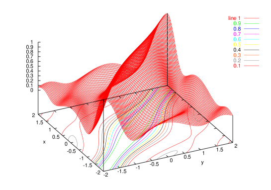
(b)

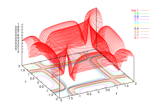
Figure 1: The square of modulus of the complex degree of coherence, $|\gamma(x,y)|^{2}$, for two “approximate complex fermion coherent states” according to Eq. (20) that differ only by the permutation $P$. The modes are forty one-dimensional monochromatic waves with equally spaced wavenumbers (“comb”) ordered according to their increasing wavenumber, and all the amplitudes $\alpha_{k}$ are chosen to be equal to $0.166$. The permutation in case (a) is identity, in case (b) a random permutation. The correlators clearly differ, which shows that the ordering of displacement operators is of large importance and different orderings result in physically different states.

One could attempt to remove the permutation dependence of Eq. (20) by averaging it over all permutations of the modes:

$$\overline{|\vec{\alpha}\rangle}=\sum_{P}|\vec{\alpha}\rangle_{P},$$ (21)

up to a normalization factor. However, the resulting state has only zero- and single-particle components because all the multi-particle parts cancel due to the fermion anticommutation relations. As the state $\overline{|\vec{\alpha}\rangle}$ contains no more than one fermion, it reduces to a single-mode “approximate complex fermion coherent state”. Thus we see that defining a multi-mode fermion coherent state using displacement operators requires an a priori mode ordering. Such an ordering, however, cannot be justified physically as none of the modes is preferred above the others.

Linear mode coupler: — Suppose that the most general single-mode fermion pure state $\beta_{0}|0\rangle+\beta_{1}|1\rangle$ is mixed with the vacuum state via linear mode coupling. The resultant output state is

$$\beta_{0}|0\rangle_{1}|0\rangle_{2}+t\beta_{1}|1\rangle_{1}|0\rangle_{2}+r\beta_{1}|0\rangle_{1}|1\rangle_{2},$$ (22)

where the indices 1, 2 label the output modes and $t$ and $r$ is the complex transmissivity and reflectivity, respectively. Evidently expression (22) cannot be written as a product of a state of the first and second output ports, respectively, unless $\beta_{1}=0$. For small $\beta_{1}$, which corresponds to the above definition of the “approximate complex fermion coherent state”, one obtains almost a product state in (22). Hence, “approximate complex fermion coherent states” approximately satisfy the linear mode coupler condition. However, the condition is satisfied exactly only by the vacuum state, that is, in the limit of no particles.

Summary: — Although the single-fermion “approximate complex coherent states” approximately satisfy the coherence requirements given above (where, by single-fermion, we mean a superposition of no fermion and one fermion with the one-fermion contribution very small), we shall see that multi-mode “approximate complex fermion coherent states” are not so accommodating. In the next section we state several important propositions that hold for normally-ordered fermion correlators and do not have direct counterparts for boson fields. Based on these results, we will show that the correlator factorization condition cannot be satisfied for “approximate complex fermion coherent states”, even approximately, except for the case of single-particle fermion states.

V Properties of normally-ordered fermion correlators

Fermion correlators are defined analogously to the boson counterparts and provide information on expected measurement outcomes by instruments at different spacetime coordinates. Definitions and examples of fermion correlators are presented in Appendix C.

In the following we prove several important propositions that hold for normally-ordered fermion correlators of an arbitrary state (pure or mixed) and that are consequences of Pauli’s exclusion principle.

Proposition 2.

For any fermion field state, the fermion correlator $\Gamma^{(n)}(x_{1},\dots,x_{n},y_{n},\dots,y_{1})$ tends to zero smoothly whenever two points $x_{i},x_{j}$ or $y_{i},y_{j}$ approach each other.

Proof.

Without lost of generality we can assume that $i=1,j=2$. Using the mode decomposition of $\hat{\psi}(x_{i})=\sum_{k}\varphi_{k}(x_{i})\hat{a}_{k}$, we obtain

$$\Gamma^{(n)} =\sum_{kl}\varphi^{*}_{k}(x_{1})\varphi^{*}_{l}(x_{2})\langle\hat{a}^{\dagger}_{k}\hat{a}^{\dagger}_{l}\hat{\psi}^{\dagger}(x_{3})\cdots\hat{\psi}^{\dagger}(x_{n})\hat{\psi}(y_{n})\cdots\hat{\psi}(y_{1})\rangle$$

$$=\frac{1}{2}\sum_{kl}[\varphi^{*}_{k}(x_{1})\varphi^{*}_{l}(x_{2})-\varphi^{*}_{l}(x_{1})\varphi^{*}_{k}(x_{2})]\langle\hat{a}^{\dagger}_{k}\hat{a}^{\dagger}_{l}\hat{\psi}^{\dagger}(x_{3})\cdots\hat{\psi}^{\dagger}(x_{n})\hat{\psi}(y_{n})\cdots\hat{\psi}(y_{1})\rangle,$$ (23)

where the anticommutation relation $\hat{a}^{\dagger}_{k}\hat{a}^{\dagger}_{l}=-\hat{a}^{\dagger}_{l}\hat{a}^{\dagger}_{k}$ was employed.

In this way, if $x_{1}\to x_{2}$, the antisymmetric function $\varphi^{*}_{k}(x_{1})\varphi^{*}_{l}(x_{2})-\varphi^{*}_{l}(x_{1})\varphi^{*}_{k}(x_{2})$ goes to zero and so does the whole correlator. The same argument can be used if some pair of points $y_{i},y_{j}$ goes together. The smoothness follows from the smoothness of the mode functions $\varphi_{k}(x)$. ∎

Proposition 2 shows that it is impossible to find two fermions at points too close to each other, which is a manifestation of Pauli’s exclusion principle.

Figure 2: The second-order correlator $|\Gamma^{(2)}(x,y,y,x)|^{2}$ for a weak “approximate complex fermion coherent state” as in Fig. 1 (a). The dip along the line $x=y$ is a common feature of this correlator regardless of the state and is a consequence of the fact that $\Gamma^{(2)}(x,y,y,x)\to 0$ when $x\to y$.

Proposition 3.

If the fermion correlator $\Gamma^{(n)}(x_{1},\dots,x_{n},y_{n},\dots,y_{1})$, for $n>1$, factorizes for some state of the fermion field, then $\Gamma^{(n)}(x_{1},\dots,x_{n},y_{n},\dots,y_{1})$ is identically equal to zero.

Proof.

The factorization of the correlator implies that

$$\Gamma^{(n)}(x_{1},\dots,x_{n},y_{n},\dots,y_{1})=f(x_{1})\cdots f(x_{n})g(y_{1})\cdots g(y_{n}).$$ (24)

However, if $x_{i}=x_{j}\,(i\not=j)$, then it follows from Proposition 2 that $\Gamma^{(n)}(x_{1},\dots,x_{n},y_{n},\dots,y_{1})=0$. Thus some of the functions $f(x),g(x)$ must be equal zero; hence $\Gamma^{(n)}(x_{1},\dots,x_{n},y_{n},\dots,y_{1})$ vanishes. ∎

Proposition 4.

Let $|\gamma(x,y)|=1$ and hence $|\Gamma(x,y)|^{2}=\Gamma(x,x)\Gamma(y,y)$ for some state $|\psi\rangle$ and a pair of points $x,y$. Then $\Gamma^{(n)}(x,y,x_{3},\dots,x_{n},y_{n},\dots,y_{1})=0$ for any $n>1$ and any $x_{3},\dots,x_{n},y_{1},\dots,y_{n}$.

Proof.

The proof is based on argument similar to the one used in Tit65 ; Tit66 for bosons in the case of the electromagnetic field. Define the operator $\hat{C}$

$$\hat{C}=\frac{1}{\sqrt{\langle\hat{\psi}^{\dagger}(x)\hat{\psi}(x)\rangle}}\,\hat{\psi}(x)-\frac{\langle\hat{\psi}^{\dagger}(y)\hat{\psi}(x)\rangle}{{\langle\hat{\psi}^{\dagger}(y)\hat{\psi}(y)\rangle}\,\sqrt{\langle\hat{\psi}^{\dagger}(x)\hat{\psi}(x)\rangle}}\,\hat{\psi}(y).$$ (25)

Thus $\langle\psi|\hat{C}^{\dagger}C|\psi\rangle=1-|\gamma(x,y)|^{2}$, which is equal to zero by assumption. It follows that $\hat{C}|\psi\rangle=0$. Hence

$$\hat{\psi}(x)|\psi\rangle=\frac{\langle\hat{\psi}^{\dagger}(y)\hat{\psi}(x)\rangle}{{\langle\hat{\psi}^{\dagger}(y)\hat{\psi}(y)\rangle}}\,\hat{\psi}(y)|\psi\rangle.$$ (26)

This equation then yields $\hat{\psi}(x)\hat{\psi}(y)|\psi\rangle=0$ because $[\hat{\psi}(y)]^{2}=0$ due to anticommutation relations. Hence, any normally-ordered correlator containing the operator product $\hat{\psi}(x)\hat{\psi}(y)$ or $\hat{\psi}^{\dagger}(x)\hat{\psi}^{\dagger}(y)$ turns into zero. In particular $\Gamma^{(n)}(x,y,\dots)=0$. ∎

One of the consequences of Proposition 4 is that whenever the field is perfectly first-order-coherent at the points $x,y$, it is impossible to find a fermion at the point $x$ and another fermion at $y$. This can be understood as another (perhaps unusual) demonstration of the Pauli exclusion principle.

Proposition 5.

Let $|\gamma(x,y)|=1$ for some state $|\psi\rangle$ for all $x,y$. Then the state has support over only the vacuum and single-particle states. That is, the probability for two fermions in the field is identically zero.

Proof.

The proof follows directly from Proposition 4. An alternative proof is based on an related result for optical field stating that if $|\gamma(x,y)|=1\,\,\forall x,y$, then only one mode of the field is occupied Tit66 . This holds also for fermions and in combination with Pauli’s principle it yields that there is at the most one fermion in the field. ∎

Impossibility of factorizing fermion correlators: — The above propositions, and Proposition 3 in particular, show that the fermion correlators of order larger than one cannot factorize except for the vacuum and single-particle states. This expresses a deep difference between boson and fermion fields: whereas the requirement of the Glauber factorization leads to coherent states for bosons, for fermions it leads to states containing zero or one particle.

Proposition 5 imposes another strong condition on the fermion field. In particular, a field with more than one fermion cannot be perfectly first-order-coherent for all $x,y$. Indeed, if for some field, $\Gamma^{(1)}(x,y)=f(x)g(y)$ holds for all $x,y$, then $|\gamma^{(1)}(x,y)|=1$. Consequently, according to Proposition 5, it follows that the field does not contain more than one fermion. Hence, even the first-order correlators cannot factorize for most fields. Importantly, even first-order correlators cannot factorize for any fermion field with support over multi-particle (even two-particle) states.

First-order correlator for “approximate complex fermion coherent states”: — To demonstrate the result from the previous section, we will now calculate the first-order correlator for the multi-mode “approximate complex fermion coherent state” (20) with $P$ the identity permutation: $P=\text{id}$. Using the decomposition $\alpha_{j}=|\alpha_{j}|\text{e}^{\text{i}\phi_{j}}$ we get:

$$\Gamma^{(1)}(x,y)= {}_{\text{id}}\langle\vec{\alpha}|\hat{\psi}^{\dagger}(x)\hat{\psi}(y)|\vec{\alpha}\rangle_{\text{id}}$$

$$= \frac{1}{4}\sum_{i,j}\varphi^{*}_{i}(x)\varphi_{j}(y)\sin(2|\alpha_{i}|)\sin(2|\alpha_{j}|)\,U_{ij}\,\text{e}^{\text{i}(\phi_{j}-\phi_{i})}+\sum_{i}\varphi^{*}_{i}(x)\varphi_{i}(y)\sin^{4}|\alpha_{i}|.$$ (27)

Here $U_{ij}$ is the product of the factors $\cos(2|\alpha_{k}|)$ with $k$ taking all values between $i$ and $j$ (with $i,j$ themselves excluded). Hence, for $i+1<j$

$$U_{ij}=\cos(2|\alpha_{{i+1}}|)\cos(2|\alpha_{{i+2}}|)\cdots\cos(2|\alpha_{{j-1}}|),$$ (28)

and for $j+1<i$ we use Eq. (28) with $i,j$ interchanged. The factor $U_{ij}$ comes from the anticommutation relations between the field operators.

If it were not for the factor $U_{ij}$ in Eq. (27), then the correlator would approximately factorize if all $|\alpha_{i}|$ were small. However, the factor $U_{ij}$ causes the correlator to be far from factorization even for small $|\alpha_{i}|$. This can be seen in Fig. 1: if $\Gamma^{(1)}(x,y)$ factorized, then the complex degree of coherence $|\gamma^{(1)}(x,y)|^{2}$ would be equal to unity. Clearly, this does not happen in Fig. 1 although the mean occupation number of each mode is very low: specifically, $(\sin|\alpha|)^{2}=0.027$. Comparing this situation with bosons where the correlation function $G^{(1)}(x,y)$ factorizes for a multi-mode coherent state, we see that there is a fundamental difference between fermions and bosons even in the limit of very low occupation numbers per mode.

The above results show that higher-order correlators cannot be factorized nontrivially for any state of the fermion field and that first-order correlators can be factorized approximately only for states containing no more than one fermion. In the case that there is truly zero or one particle, we expect the features of fermions to be the same as those of bosons because at least two particles are required to see manifestations of their quantum statistics. However, higher-order correlators that describe two- or multi-particle characteristics of the field do reveal the fundamental difference between fermions and bosons regardless of how weak the field is because the correlator tells us about the correlation statistics regardless of how rare the multi-particle events are. This is further demonstrated in Appendix D on an example of boson and fermion chaotic states.

Hence we see that there are no fermion states with complex parametrization that would, at least approximately, factorize fermion correlators, with the exception of single-particle states. Thus the definition of coherent states in terms of correlator factorization does not yield reasonable approximate multi-particle fermion coherent states, similarly as the previous definitions.

VI Conclusion

Constructions of complex fermion coherent states, or approximations to such states, is problematic, as we have shown in this paper. We have seen that multi-mode “approximate coherent states”, whether obtained as displaced vacua or as near-eigenstates of the annihilation operator, exhibit inconsistencies due to inequivalences under permutation of modes, and also do not factorize fermion correlation functions. The only fermion states that approximately satisfy the coherent state definitions are the single-mode “approximate coherent states” that contain, however, no more than one particle.

These problems arise ultimately from Pauli’s exclusion principle and the corresponding mathematical framework of anticommuting operators. The ambiguity of mode ordering, the complications of linear mode coupling, and the unfactorizability of the correlation functions are due to the exclusion principle. On the other hand, for states that contain no more than one particle, the Pauli principle has no effect and “approximate coherent states” can be defined in the subspace of the Hilbert space spanned by zero- and single-particle states. In this domain of the Hilbert space, there is no essential difference between fermions and bosons as single particles cannot manifest their distinct quantum statistics. Hence single-mode “approximate complex fermion coherent states” approximately satisfy the coherence properties in the same way as “approximate boson coherent states”, which are obtained from weak boson coherent states by truncating the particle number beyond one.

It therefore appears that the use of Grassmann numbers, which obviate the problem of anticommuting operators but introduce an unphysical parametrization, are needed to create self-consistent fermion coherent states that satisfy the expected coherence properties Cah99 ; complex parametrized fermion coherent states do not appear to be useful, even approximately.

Appendix A Mode ordering for mixtures of number states

A mixture of fermion number states does not suffer from the permutation ambiguity described in Sec. II, Eqs. (9) and (10). Indeed, the projector to a number state is invariant with respect to changes of the mode ordering due to the doubled number of the minus signs arising from the field operator anticommutation relations. For example,

$$\hat{P}_{(1_{1}1_{2})} =|1_{1}1_{2}\rangle\langle 1_{2}1_{1}|=\hat{a}_{1}^{\dagger}\hat{a}_{2}^{\dagger}|0_{1}0_{2}\rangle\langle 0_{2}0_{1}|\hat{a}_{2}\hat{a}_{1}$$ (29)

$$\hat{P}_{(1_{2}1_{1})} =|1_{2}1_{1}\rangle\langle 1_{1}1_{2}|=\hat{a}_{2}^{\dagger}\hat{a}_{1}^{\dagger}|0_{1}0_{2}\rangle\langle 0_{2}0_{1}|\hat{a}_{1}\hat{a}_{2}$$ (30)

$$\hat{P}_{(1_{1}1_{2})} =\hat{P}_{(1_{2}1_{1})}$$ (31)

It follows that also an arbitrary mixture of number state projectors, e.g. a chaotic state, is immune with respect to the change in ordering the modes. This is a contrast to superpositions of number states, for which the ambiguity is present and changing the mode ordering can lead to a physically different state, as is discussed in Sec. IV.

Appendix B Proof of equivalence of definitions of boson coherent state

Here we prove that all the four definitions of boson coherent state mentioned in Sec. III are equivalent. We denote the properties as follows,
(a) boson coherent state is an eigenstate of the annihilation operator,
(b) boson coherent state is a displaced vacuum state $|\alpha\rangle=\text{e}^{\alpha\hat{a}^{\dagger}-\alpha^{*}\hat{a}}\,|0\rangle\equiv\hat{D}(\alpha)\,|0\rangle$
(c) boson coherent state is a pure state that yields a product state when mixed with the vacuum state on a linear mode coupler (linear mode coupler).
(d) boson coherent state is a state for which all normally-ordered correlators factorize.

We will show now the implications (a) $\Rightarrow$ (c), (c) $\Rightarrow$ (b), (b) $\Rightarrow$ (a), and (a) $\Rightarrow$ (d). To show the implication (d) $\Rightarrow$ (a) is not so easy and for the proof we refer to the paper Tit66 .

First we will show (a) $\Rightarrow$ (c). Let us denote the annihilation operators of the input and output ports of the linear mode coupler by $\hat{a}_{1},\hat{a}_{2}$ and $\hat{a}_{1}^{\prime},\hat{a}_{2}^{\prime}$, respectively. The relation between $\hat{a}_{1},\hat{a}_{2}$ and $\hat{a}_{1}^{\prime},\hat{a}_{2}^{\prime}$ is

$$\hat{a}_{i}^{\prime}=\sum_{j=1}^{2}A_{ij}\hat{a}_{j}$$ (32)

with $A_{ij}$ a unitary matrix. Let an eigenstate $|\alpha\rangle$ of $\hat{a}_{1}$ incide on the first linear mode coupler input port, and vacuum incide on the second input port, which is an eigenstate of $\hat{a}_{2}$ with eigenvalue zero. It then follows from Eq. (32) that the linear mode coupler output state is an eigenstate of $\hat{a}_{1}^{\prime}$ and $\hat{a}_{2}^{\prime}$, which is a product state of the linear mode coupler outputs.

Next we show (c) $\Rightarrow$ (b): Let the boson coherent state incident on linear mode coupler be expressed in the Fock basis as follows:

$$|\alpha\rangle=\sum_{n=0}^{\infty}c_{n}(\hat{a}^{\dagger})^{n}|0\rangle$$ (33)

The series $\sum_{n=0}^{\infty}c_{n}(\hat{a}^{\dagger})^{n}$ formally defines a function of the creation operator $\hat{a}^{\dagger}$ that we will denote by $f(\hat{a}^{\dagger})$. The linear mode coupler input state is then $f(\hat{a}_{1}^{\dagger})|0\rangle$ as there is vacuum at the second input port. The relation between $\hat{a}_{1}^{\dagger},\hat{a}_{2}^{\dagger}$ and $\hat{a}_{1}^{\dagger}{}^{\prime},\hat{a}_{2}^{\dagger}{}^{\prime}$ following from Eq. (32) is $\hat{a}_{i}^{\dagger}=\sum_{j=1}^{2}A_{ji}\hat{a}_{j}^{\dagger}{}^{\prime}$. Therefore the output linear mode coupler state is $f(A_{11}\hat{a}_{1}^{\dagger}{}^{\prime}+A_{12}\hat{a}_{2}^{\dagger}{}^{\prime})|0\rangle$. According to our assumption, this is a product state of output modes $1^{\prime},2^{\prime}$, so it must hold

$$f(A_{11}\hat{a}_{1}^{\dagger}{}^{\prime}+A_{12}\hat{a}_{2}^{\dagger}{}^{\prime})=g(\hat{a}_{1}^{\dagger}{}^{\prime})h(\hat{a}_{2}^{\dagger}{}^{\prime})$$ (34)

with $g,h$ some functions. As $\hat{a}_{1}^{\dagger}{}^{\prime}$ and $\hat{a}_{2}^{\dagger}{}^{\prime}$ commute, we can treat $f,g,h$ as ordinary functions of, say, arguments $x$ and $y$ instead of $\hat{a}_{1}^{\dagger}$ and $\hat{a}_{2}^{\dagger}$. Then, denoting $F(z)=\ln f(z)$, making logarithm of Eq. (34) and performing the derivative $\partial^{2}/\partial x\,\partial y$, we arrive at the condition

$$A_{11}A_{12}F^{\prime\prime}(A_{11}x+A_{12}y)=0.$$ (35)

For both $A_{11}$ and $A_{12}$ different from zero (the opposite would correspond to a trivial linear mode coupler—either doing nothing or interchanging the modes 1 and 2), this is possible only if $F$ is a linear function, i.e., if $F(z)=\lambda z+\gamma$. It then follows that $f(\hat{a}^{\dagger})=\text{e}^{\lambda\hat{a}^{\dagger}+\gamma}$. However, then $f(\hat{a}_{1}^{\dagger})|0\rangle$ is a displaced vacuum state (up to a normalization constant) because the Campbell-Hausdorff-Baker formula yields

$$\text{e}^{\lambda\hat{a}^{\dagger}+\gamma}|0\rangle=\text{e}^{|\lambda|^{2}/2+\gamma}\text{e}^{\lambda\hat{a}^{\dagger}-\lambda^{*}\hat{a}}|0\rangle=\text{e}^{|\lambda|^{2}/2+\gamma}\hat{D}(\lambda)|0\rangle.$$ (36)

To show (b) $\Rightarrow$ (a) means to show that $\hat{D}(\alpha)|0\rangle$ is an eigenstate of the annihilation operator. Displacing the annihilation operator, we have

$$\hat{a}\hat{D}(\alpha)|0\rangle=\hat{D}(\alpha)\hat{D}^{\dagger}(\alpha)\hat{a}\hat{D}(\alpha)|0\rangle=\hat{D}(\alpha)(\hat{a}+\alpha\openone)|0\rangle=\alpha\hat{D}(\alpha)|0\rangle,$$ (37)

which we wanted to prove.

Next we show (a) $\Rightarrow$ (d): The field operators $\hat{\psi}(x)$ and $\hat{\psi}^{\dagger}(x)$ are linear combinations of single-mode annihilation operators $\hat{a}_{i}$ and creation operators $\hat{a}^{\dagger}_{i}$, respectively. Any (possibly multi-mode) coherent state is therefore a right eigenstate of $\hat{\psi}(x)$ and left eigenstate of $\hat{\psi}^{\dagger}(x)$. From this the factorization (16) follows immediately.

Appendix C Normally-ordered correlators

Correlators are important tools for describing coherence of both boson and fermion fields. They are defined as expectation values of products of creation and annihilation operators at different space-time points.

The fermion correlators of the $n^{\rm th}$ order are defined by analogy to their boson counterparts

$$\Gamma^{(n)}(x_{1},\dots,x_{n},y_{n},\dots,y_{1})\equiv\langle\hat{\psi}^{\dagger}(x_{1})\cdots\hat{\psi}^{\dagger}(x_{n})\hat{\psi}(y_{n})\cdots\hat{\psi}(y_{1})\rangle$$ (38)

(we use the Greek letter $\Gamma$ to distinguish from the boson correlator $G$). Of particular importance is the correlator with repeated arguments, for which we introduce the shorter expression $\Gamma^{(n)}(x_{1},\dots,x_{n})\equiv\Gamma^{(n)}(x_{1},\dots,x_{n},x_{n},\dots,x_{1})$, which corresponds to the $n$-fermion detection probability, and also the one-fermion cross-correlator $\Gamma(x,y)\equiv\Gamma^{(1)}(x,y)$.

The normalized first-order cross-correlator $\gamma(x,y)=\Gamma(x,y)/\sqrt{\Gamma(x,x)\Gamma(y,y)}$ is called complex degree of coherence and its magnitude expresses the visibility of interference fringes in a double-slit experiment in which the two slits are placed at the points $x$ and $y$, respectively Man95 . If $|\gamma(x,y)|=1$ for all $x,y$, we say that the field has perfect first-order coherence.

Appendix D Correlators for boson and fermion chaotic states

We will show now that for chaotic states, the fermion or boson nature of the particles does not have an effect on the first-order correlator while it has a strong effect on the higher-order correlators.

For a chaotic state Gla70 , each mode of the chaotic field has maximum entropy for a given mean number of particles in this mode, and the density operator of the field is a direct product of single-mode density operators. This second property simply implies that, in the chaotic state, the individual modes of the field are totally uncorrelated.

The chaotic state density operator of a single mode of bosons or fermions with mean number of particles $M$ can be expressed as

$$\hat{\rho}=\frac{\text{e}^{-\xi\hat{a}^{\dagger}\hat{a}}}{\text{Tr}\,(\text{e}^{-\xi\hat{a}^{\dagger}\hat{a}})},$$ (39)

with

$$\text{e}^{-\xi}=\frac{M}{1+M},\;\text{Tr}\,(\text{e}^{-\xi\hat{a}^{\dagger}\hat{a}})=1+M$$ (40)

for bosons and

$$\text{e}^{-\xi}=\frac{M}{1-M},\;\text{Tr}\,(\text{e}^{-\xi\hat{a}^{\dagger}\hat{a}})=\frac{1}{1-M}$$ (41)

for fermions (unlike previous sections, here we denote the fermion field operators by $\hat{a},\hat{a}^{\dagger}$ rather than $\hat{c},\hat{c}^{\dagger}$ for compact notation). Thus we have the density operators for bosons and fermions in the following forms:

$$\hat{\rho}_{\rm B}=\frac{1}{1+M}\sum_{n=0}^{\infty}\left(\frac{M}{1+M}\right)^{n}\,|n\rangle\langle n|,\qquad\hat{\rho}_{\rm F}=(1-M)\sum_{n=0}^{1}\left(\frac{M}{1-M}\right)^{n}\,|n\rangle\langle n|$$ (42)

Consider now a multi-mode chaotic field of bosons or fermions. Let there be $N$ occupied modes labeled by $1,\dots,N$ and let the mean number of particles in the $i^{\text{th}}$ mode be $M_{i}$. For brevity, we denote the boson and fermion correlators by $G_{\rm B}$ and $G_{\rm F}$, respectively, in this section. The first order cross-correlator $G_{\text{B,F}}^{(1)}(x,y)$ can readily be calculated and has the same form for bosons and fermions:

$$G_{\rm B,F}^{(1)}(x,y)=\sum_{i=1}^{N}M_{i}\varphi_{i}^{*}(x)\varphi_{i}(y)$$ (43)

Eq. (43) shows that the first order coherence (which is related to the visibility of interference fringes) for chaotic states is not at all influenced by the fermion or boson nature of the particles, provided the mean occupation numbers are the same. This can be expected as the first order correlator is not related to multi-particle correlations so it should not be affected by the exchange interaction.

The $n^{\text{th}}$-order correlator can also be calculated for the chaotic state. The following formula holds exactly for fermions and for bosons it holds with good accuracy if $M_{i}\ll 1,i=1,\dots,N$:

$$G_{\rm B,F}^{(n)}(x_{1},\dots,x_{n},y_{n},\dots,y_{1})=\sum_{P}\chi_{\rm B,F}^{{\rm par}(P)}G_{\rm B,F}^{(1)}(x_{1},y_{P^{(1)}})G_{\rm B,F}^{(1)}(x_{2},y_{{P}^{(2)}})\cdots G_{\rm B,F}^{(1)}(x_{n},y_{P^{(n)}})$$ (44)

Here the sum runs over all permutations $P$ of the indices $1,2,\dots,n$, the parity of the permutation $P$ is denoted by ${\rm par}(P)$, and $\chi_{\rm B}=1$, $\chi_{\rm F}=-1$ is the boson and fermion sign factor, respectively. Hence the higher-order correlators are no longer identical for boson and fermion chaotic states, which is manifested as bunching (antibunching) for boson (fermion) chaotic fields. If $x_{i}\to x_{j},i\not=j$, $G_{\rm F}$ goes to zero according to Eq. (44) due to the factor $(-1)^{{\rm par}(P)}$, which is in agreement with the general property of fermion correlators (Proposition 2).

References

- (1) A. I. Signal and U. Zülicke, Appl. Phys. Lett. 87, 102102 (2005)
- (2) E. C. G. Sudarshan, Phys. Rev. Lett. 10, 277 (1963).
- (3) R. J. Glauber, Phys. Rev. 130, 2529 (1963).
- (4) R. J. Glauber, Phys. Rev. 131, 2766 (1963).
- (5) J. R. Klauder, Phys. Rev. Lett. 16, 534 (1966).
- (6) J. L. Martin, Proc. Roy. Soc. Lond. A 251, 543 (1959); Y. Ohnuki and T. Kashiwa, Prog. Theor. Phys. 60, 548 (1978); J. R. Klauder and B.-S. Skagerstam, Coherent States (World Scientific, Singapore, 1985).
- (7) F. A. Berezin, The Method of Second Quantization (Academic Press, New York, 1966).
- (8) J. Schwinger, Phys. Rev. 92, 1283 (1953).
- (9) K. E. Cahill and R. J. Glauber, Phys. Rev. A 59, 1538 (1999).
- (10) U. M. Titulaer and R. J. Glauber, Phys. Rev. 140, B676 (1965).
- (11) U. M. Titulaer and R. J. Glauber, Phys. Rev. 145, 1041 (1966).
- (12) H. P. Yuen and J.H. Shapiro, in Coherence and Quantum Optics IV, edited by L. Mandel and E. Wolf (Plenum, New York, 1978), p. 719.
- (13) T. Tyc and B. C. Sanders, J. Phys. A: Math. Gen. 37, 7341 (2004).
- (14) L. Mandel and E. Wolf, Optical Coherence and Quantum Optics (Cambridge University Press, Cambridge, 1995).
- (15) R. Glauber, in Quantum Optics, edited by S. Kay and A. Maitland. (Academic Press, New York, 1970), p. 53.
- (16) Y. Aharonov, D. Falkoff, E. Lerner, and H. Pendleton, Ann. Phys. (N.Y.) 39, 498 (1966).