Quantum Searching amidst Uncertainty

Abstract

Consider a database most of whose entries are marked but the precise fraction of marked entries is not known. What is known is that the fraction of marked entries is $1-\epsilon$, where $\epsilon$ is a random variable that is uniformly distributed in the range $\left(0,\epsilon_{0}\right).$The problem is to try to select a marked item from the database in a single query. If the algorithm selects a marked item, it succeeds, else if it selects an unmarked item, it makes an error.

How low can we make the probability of error? The best possible classical algorithm can lower the probability of error to $O\left(\epsilon_{0}^{2}\right).$ The best known quantum algorithms for this problem could also only lower the probability of error to $O\left(\epsilon_{0}^{2}\right).$ Using a recently invented quantum search technique, this paper gives an algorithm that reduces the probability of error to $O\left(\epsilon_{0}^{3}\right).$ The algorithm is asymptotically optimal.

1 Introduction

Classical search algorithms are robust. If we reduce the problem size, the algorithm has fewer items to search and the performance of the algorithm will almost always improve. Quantum search algorithms depend on delicate interference effects, any change in parameters leads to significantly different results. For example, if we reduce the number of states in the database by a factor of four, a quantum search algorithm that would have previously succeeded, will now fail with certainty. Quantum algorithms usually exhibit oscillatory behavior in their performance characteristics. As a result of this, if there is some quantity that we want to maximize, e.g. the probability of the system being in marked states, we will need very precise knowledge of the problem parameters. Given such knowledge, it is easy to fine-tune the algorithm so that it achieves a probability of success of unity. What happens if we do not have this knowledge? This can be a serious handicap for a quantum search algorithm. This paper describes a way around this problem.

The original quantum search algorithm [1] considered the problem of finding a marked item in a large unsorted database with minimum queries to the database. For this type of problem it is usually enough to be able to obtain the correct answer with a constant probability since the procedure can be repeated a logarithmic number of times to drive the probability exponentially close to unity. In that problem a logarithmic factor was not significant since the quantum search algorithm gave a square-root asymptotic improvement. However there are other important problems where the additional queries create a significant overhead and need to be minimized, e.g. when we are limited to a single query and have to find the answer with a probability approaching unity. One field in which this type of problem occurs is in pattern recognition and image analysis where each query requires a lot of signal processing and the consequences of making an error are catastrophic.

2 The problem

Consider the situation where a large fraction of the items in a database are marked, but the precise fraction of marked items is not known. The goal is to find a single marked item with as high a probability as possible in a single query to the database. For concreteness, say some unknown fraction $(1-\epsilon)$ of the items are marked, with $\epsilon$ uniformly distributed  in the range $\left(0,\epsilon_{0}\right)$ with equal probability. The search algorithm returns an item, if it is a marked item the algorithm is said to succeed, else if it is unmarked, the algorithm is said to fail.

Classically the smallest error that can be obtained is $O\left(\epsilon_{0}^{2}\right)$. To achieve this, uniformly guess an input and evaluate the function. If the function outputs 1, you’re done, otherwise guess again and cross your fingers (because you have no more evaluations left). One cannot do better than $O\left(\epsilon_{0}^{2}\right)$ classically. In this paper we show that the probability of failure for the new scheme is $O\left(\epsilon_{0}^{3}\right),$ whereas that of the best (possible) classical scheme and that of the best known quantum schemes are both $O\left(\epsilon_{0}^{2}\right)$.

Before considering the specific problem mentioned above, let us describe a general framework. Consider the following transformation

$$UR_{s}U^{\dagger}R_{t}U\left|s\right\rangle$$ (1)

$$R_{s} =I-(1-\exp\left(i\frac{\pi}{3}\right))\left|s\right\rangle\left\langle s\right|,\ \ \ R_{t}=I-(1-\exp\left(i\frac{\pi}{3}\right))\left|t\right\rangle\left\langle t\right|$$

$U$ is an arbitrary unitary transformation, $R_{t}$ & $R_{s}$ denote selective phase shifts of the respective state(s) by $\frac{\pi}{3}.$ Note that if we were to change these phase shifts from $\frac{\pi}{3}$ to $\pi,$ we would get one iteration of the amplitude amplification algorithm [2], [3].

The next section shows that if $U$ drives the state vector from a source $\left(s\right)$ to a target $\left(t\right)$ state with a probability of $\left(1-\epsilon\right)$, i.e. $\left\|U_{ts}\right\|^{2}=\left(1-\epsilon\right)$, then the transformation (1) drives the state vector from the source to the same target state with a probability of $\left(1-\epsilon^{3}\right).$ The deviation from the $t$ state has hence fallen from $\epsilon$ to $\epsilon^{3}$. Note that this is different from the amplitude amplification framework where the amplitudes were getting amplified; over here it is more convenient to present the results in terms of the probabilities.

The striking aspect of this result is that it holds for any kind of deviation from the $t$ state. Unlike the standard search (or amplitude amplification) algorithm which would greatly overshoot the target state when $\epsilon$ is small (Figure 1); the new algorithm will always move towards the target. As shown in Section 5, this feature of the framework can be used to develop algorithms that are more robust to variations in the problem parameters.

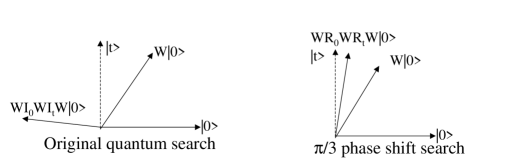
Figure 1: The original quantum search algorithm is very sensitive to the fraction of marked states. For example, when the fraction is about 3/4, the algorithm fails, the algorithm of this paper will always produce an improvement.

3 Analysis

We analyze the effect of the transformation $UR_{s}U^{\dagger}R_{t}U$ when it is applied to the $\left|s\right\rangle$ state. As mentioned in the previous section, $R_{t}$ & $R_{s}$ denote selective phase shifts of the respective state(s) by $\frac{\pi}{3}$ ($t$ for target, $s$ for source). We show that if $\left\|U_{ts}\right\|^{2}=\left(1-\epsilon\right),$ then

$$\left\|\left\langle t\right|UR_{s}U^{\dagger}R_{t}U\left|s\right\rangle\right\|^{2}=\left(1-\epsilon^{3}\right).$$ (2)

In the rest of this section, the greek alphabet $\theta$ will be used to denote $\frac{\pi}{3}.$ Start with $\left|s\right\rangle$ and apply the operations $U,R_{s},U^{\dagger},R_{t}$ &$\ U.$ If we analyze the effect of the operations, one by one, just as in the original quantum search algorithm [1], we find that it leads to the following superposition (this calculation is carried out in the appendix):

$$U\left|s\right\rangle\left(e^{i\theta}+\left\|U_{ts}\right\|^{2}\left(e^{i\theta}-1\right)^{2}\right)+\left|t\right\rangle U_{ts}\left(e^{i\theta}-1\right).$$

To calculate the deviation of this superposition from $\left|t\right\rangle$, consider the amplitude of the above superposition in non-target states. The probability is given by the absolute square of the corresponding amplitude:

$$\left(1-\left\|U_{ts}\right\|^{2}\right)\left\|\left(e^{i\theta}+\left\|U_{ts}\right\|^{2}\left(e^{i\theta}-1\right)^{2}\right)\right\|^{2}.$$

Substituting $\left\|U_{ts}\right\|^{2}=\left(1-\epsilon\right),$ the above quantity becomes$:$

$$\epsilon\left\|\left(e^{i\theta}+\left(1-\epsilon\right)\left(e^{i\theta}-1\right)^{2}\right)\right\|^{2}$$

$$=\epsilon\left\|\left(-e^{i\theta}+e^{2i\theta}+1\right)-\epsilon\left(e^{i\theta}-1\right)^{2}\right\|^{2}$$

$$=\epsilon^{3}.$$

4 Existing Algorithms

4.1 Classical Algorithm

The best classical algorithm is to select a random state and see if it is a $t$ state (one query). If yes, return this state; if not, pick another random state and return that without any querying. Note that this algorithm requires a single query, not two. The probability of failure is equal to that of not getting a single $t$ state in two random picks since if either of the two states is a marked state, the algorithm will succeed. This probability is equal to $\epsilon^{2}.$ Since $\epsilon$ is uniformly distributed in the range $\left(0,\epsilon_{0}\right)$. The overall failure probability becomes$\frac{\int_{0}^{\epsilon_{0}}\epsilon^{2}d\epsilon}{\int_{0}^{\epsilon_{0}}d\epsilon}=\frac{1}{3}\epsilon_{0}^{2}$

Figure 2: By setting the six-state ancilla, b, to the superposition $\frac{1}{\sqrt{6}}\left(\left|0\right\rangle+\left|1\right\rangle\omega+\left|2\right\rangle\omega^{2}+\left|3\right\rangle\omega^{3}+\left|4\right\rangle\omega^{4}+\left|5\right\rangle\omega^{5}\right)$ where $\omega=\exp\left(-\frac{i\pi}{3}\right),$ we get a $\frac{\pi}{3}$ phase-shift of the states for which $F(x)=1$ relative to those for which $F\left(x\right)=0.$ [10] gives a technique for implementing this with qubits.

4.2 Quantum Searching

Boyer, Brassard, Høyer and Tapp [4] first described in detail an algorithm that succeeds with probability approaching 1, regardless of the number of solutions (it’s a classical algorithm that uses quantum searching as a subroutine; of course, it can be made fully quantum.) The first quantum algorithm to be able to search in a single query with a success probability approaching 1 was given by Mosca [5].

Mosca observed that the quantum counting algorithm of [4] (based on the original searching algorithm) produces a solution with probability converging to $1/2$. One easily converts this to an algorithm with probability of success converging to $1/4$. Thus by using this algorithm as a sub-routine in another quantum search, we get success probability converging to $1$. (This appears to be based on the observation in [4] that an algorithm that succeeds with probability exactly $1/4$ can be amplified to one with success probability exactly $1$ using only one quantum search iterate). In other words, the technique Mosca uses is to take a search algorithm that succeeds with probability $1/4-X$ and then use one quantum search iteration to map it to an algorithm that succeeds with probability $\left(1-12X^{2}-16X^{3}\right)$. Using this scheme, if the fraction of marked states of the database is $1-\epsilon$, one can easily obtain a marked state with a probability of error of $1-\frac{3}{4}\epsilon^{2}-\frac{1}{4}\epsilon^{3}$ by means of a single quantum query. The overall failure probability in this case becomes $\frac{\int_{0}^{\epsilon_{0}}\left(\frac{3}{4}\epsilon^{2}+\frac{1}{4}\epsilon^{3}\right)d\epsilon}{\int_{0}^{\epsilon_{0}}d\epsilon}=\frac{1}{4}\epsilon_{0}^{2}+\frac{1}{16}\epsilon_{0}^{3}$

A recent quantum search based algorithm for this problem is by Younes et al [6] (actually it is somewhat unfair to compare it to the other algorithms since this was specifically designed to perform well when the success probability was close to $\frac{1}{2},$ not close to $1)$. This finds a solution with a probability of $\left(1-\cos\theta\right)\left(\frac{\sin^{2}\left(q+1\right)\theta}{\sin^{2}\theta}+\frac{\sin^{2}q\theta}{\sin^{2}\theta}\right),$ where $q$ = number of queries and $\theta=\arccos\epsilon$ ((59) from [6]). When $q=1,$ the success probability becomes: $\left(1-\epsilon\right)\left(1+4\epsilon^{2}\right),$ hence the probability of error becomes $\epsilon-4\epsilon^{2}+4\epsilon^{3}$. The overall failure probability becomes $\frac{\int_{0}^{\epsilon_{0}}\left(\epsilon-4\epsilon^{2}+4\epsilon^{3}\right)d\epsilon}{\int_{0}^{\epsilon_{0}}d\epsilon}=\left(\frac{1}{2}\epsilon_{0}-\frac{4}{3}\epsilon_{0}^{2}+\epsilon_{0}^{3}\right)$

5 New algorithm

As in the quantum search algorithm, encode the $N$ items in the database in terms of $\log_{2}N$ qubits. The algorithm consists of applying the transformation $WR_{\overline{0}}WR_{t}W$ to $\left|\overline{0}\right\rangle$. W is the Walsh-Hadamard Transformation and $\overline{0}$ is the state with all qubits in the $0$ state. After this an observation is made which makes the system collapse into a basis state.

In order to analyze the performance of this algorithm, note that the algorithm is merely the phase shift transformation $UR_{s}U^{\dagger}R_{t}U$ applied to  $\left|s\right\rangle$ which has already been analyzed in section 3. $U$ is the W-H transform ($W$) and the state $s$ is the $\overline{0}$ state (state with all qubits in the 0 state), then $\left\|U_{ts}\right\|^{2}=1-\epsilon,$ where $\epsilon$ lies in the range $\left(0,\epsilon_{0}\right).$ Therefore after applying the transformation $WR_{\overline{0}}WR_{t}W$ to $\left|\overline{0}\right\rangle$ , the probability of being in a non-$t$ state becomes $\epsilon^{3}$, i.e. the overall failure probability becomes $\frac{\int_{0}^{\epsilon_{0}}\epsilon^{3}d\epsilon}{\int_{0}^{\epsilon_{0}}d\epsilon}=\frac{1}{4}\epsilon_{0}^{3}$

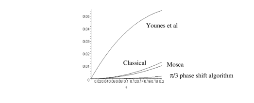
Figure 3: Comparison of the failure probability of the $\pi/3$ phase shift algorithm with a classical algorithm, [6], and [5], when the fraction of unmarked states $\epsilon$, varies between 0 & 0.2.

The performance of the algorithm is graphically illustrated in Figure 3.

6 Extensions

6.1 Multi-query searching

In practice, a database search would use multiple queries. The technique discussed above extends neatly to the multi-query situation. As described in [7], the multi-query algorithm based on the $\frac{\pi}{3}$ phase-shift transformation is able to reduce the probability of error to $\frac{\epsilon_{0}^{2q+1}}{2q+2}$ after $q$ queries to the database. A classical algorithm reduces the probability of error to $\frac{\epsilon_{0}^{q+1}}{q+2}.$ Note that $q=1$ gives the same results as in section 5.

6.2 Optimality

Both the single query, as well as the multi-query algorithms are asymptotically optimal in the limit of small $\epsilon_{0}$. This is separately proved in [9].

6.3 Quantum Control & Error Correction

Connections to control and error correction might be evident. Let us say that we are trying to drive a system from an $s$ to a $t$ state/subspace. The transformation that we have available for this is $U$ which drives it from $s$ to $t$ with a probability $\left\|U_{ts}\right\|^{2}$ of $\left(1-\epsilon\right),$ i.e. the probability of error in this transformation is $\epsilon$. Then the composite transformation $UR_{s}U^{\dagger}R_{t}U$ will reduce the error to $\epsilon^{3}.$

This technique is applicable whenever the transformations $U,\ U^{\dagger},R_{s}\ \&\ R_{t}$ can be implemented. This will be the case when errors are systematic errors or slowly varying errors, e.g. due to environmental degradation of some component. This would not apply to errors that come about as a result of sudden disturbances from the environment. It is further assumed that the transformation $U$ can be inverted with exactly the same error. Traditionally quantum error correction is carried out at the single qubit level where individual errors are corrected, each error being corrected in a separate way. With the machinery of this paper, errors can be corrected without ever needing to identify the error syndrome. This is discussed in [7] and [8].

7 Appendix

We analyze the effect of the transformation (3) of section 3 when it is applied to the $\left|s\right\rangle$ state. As in section 3, $\theta$ will denote $\frac{\pi}{3}.$ We show that if $\left\|U_{ts}\right\|^{2}=\left(1-\epsilon\right),$ then

$$\left\|\left\langle t\right|UR_{s}U^{{}^{{}^{{\dagger}}}}R_{t}U\left|s\right\rangle\right\|^{2}=\left(1-\epsilon^{3}\right)$$ (3)

starting state

$\left|s\right\rangle\qquad\qquad\qquad\qquad\qquad\qquad\qquad\qquad\qquad\qquad\qquad\qquad\qquad\qquad\qquad\qquad\qquad\qquad\qquad\qquad\qquad\qquad\qquad\qquad\qquad\qquad\qquad\qquad\qquad\qquad\qquad\qquad\qquad\qquad\qquad\qquad\qquad\qquad\qquad\qquad\qquad\qquad\qquad\qquad$

after $R_{t}U$

$$R_{t}U\left|s\right\rangle=U_{ts}\left(e^{i\theta}-1\right)\left|t\right\rangle+U\left|s\right\rangle$$

after $U^{{}^{{}^{{\dagger}}}}:$

$$U^{{}^{{}^{{\dagger}}}}R_{t}U\left|s\right\rangle=\left|s\right\rangle+U_{ts}\left(e^{i\theta}-1\right)U^{{}^{{}^{{\dagger}}}}\left|t\right\rangle$$

after $R_{s}$

$:$

$$R_{s}U^{{}^{{}^{{\dagger}}}}R_{t}U\left|s\right\rangle =\left(\left|s\right\rangle+U_{ts}\left(e^{i\theta}-1\right)U^{{}^{{}^{{\dagger}}}}\left|t\right\rangle\right)$$

$$+\left(e^{i\theta}-1\right)\left(\left|s\right\rangle+U_{ts}\left(e^{i\theta}-1\right)\left|s\right\rangle\left\langle s\right|U^{{}^{{}^{{\dagger}}}}\left|t\right\rangle\right)$$

$$=\left|s\right\rangle\left(e^{i\theta}+\left\|U_{ts}\right\|^{2}\left(e^{i\theta}-1\right)^{2}\right)+U_{ts}\left(e^{i\theta}-1\right)U^{{}^{{}^{{\dagger}}}}\left|t\right\rangle$$

after the final $U$:

$$UR_{s}U^{{}^{{}^{{\dagger}}}}R_{t}U\left|s\right\rangle=U\left|s\right\rangle\left(e^{i\theta}+\left\|U_{ts}\right\|^{2}\left(e^{i\theta}-1\right)^{2}\right)+U_{ts}\left(e^{i\theta}-1\right)\left|t\right\rangle$$

Calculating the error

To estimate the error, consider the amplitude of the above superposition in non-target states (this is due to the portion $U\left|s\right\rangle\left(e^{i\theta}+\left\|U_{ts}\right\|^{2}\left(e^{i\theta}-1\right)^{2}\right),$ the other portion $U_{ts}\left(e^{i\theta}-1\right)\left|t\right\rangle$ is clearly in the target state). The magnitude of the error probability is given by the absolute square of this error amplitude:

$$\left(1-\left\|U_{ts}\right\|^{2}\right)\left\|\left(e^{i\theta}+\left\|U_{ts}\right\|^{2}\left(e^{i\theta}-1\right)^{2}\right)\right\|^{2}$$

Assume $\left\|U_{ts}\right\|^{2}$ to be $\left(1-\epsilon\right),$ the above quantity becomes$:$

$$\epsilon\left\|\left(e^{i\theta}+\left(1-\epsilon\right)\left(e^{i\theta}-1\right)^{2}\right)\right\|^{2}$$

$$=\epsilon\left\|\left(-e^{i\theta}+e^{2i\theta}+1\right)-\epsilon\left(e^{i\theta}-1\right)^{2}\right\|^{2}$$

$$=\epsilon^{3}$$

References

- [1] L. K. Grover, “Quantum Mechanics helps in searching for a needle in a haystack”, Phys. Rev. Letters, 78(2), 325, 1997.
- [2] G. Brassard and P. Hoyer, ”An exact quantum polynomial-time algorithm for Simon’s problem”, Proceedings of Fifth Israeli Symposium on Theory of Computing and Systems (ISTCS’97), Ramat-Gan, Israel, June 1997, 12–23, quant-ph/9704027.
- [3] L. K. Grover, “Quantum computers can search rapidly by using almost any transformation”, Phys. Rev. Letters, 80(19), 1998, 4329-4332.
- [4] Boyer et al, quant-ph/9605034, PhysComp 96, and Fortsch.Phys. 46 (1998) 493-506.
- [5] M. Mosca, Theoretical Computer Science, 264 (2001) pages 139-153.
- [6] Ahmed Younes, Jon Rowe, Julian Miller, ”Quantum Search Algorithm with more Reliable Behavior using Partial Diffusion,” quant-ph/0312022.
- [7] Lov K. Grover, ”A different kind of quantum search”, quant-ph/0503205.
- [8] B. Reichardt & L.K. Grover, ”Quantum error correction of systematic errors using a quantum search framework,” quant-ph/0506242 .
- [9] Sourav Chakraborty, Jaikumar Radhakrishnan, Nanda Raghunathan, ”The optimality of Grover’s recent quantum search algorithm,” manuscript in preparation.
- [10] Tathagat TulsiTathagat Tulsi, Lov Grover, Apoorva Patel, ”A new algorithm for directed quantum search,” quant-ph/0505007.