Quantum Electrodynamics near a Dielectric Half-space

Abstract

We determine the photon propagator in the presence of a non-dispersive dielectric half-space and use it to calculate the self-energy of an electron near a dielectric surface.

I Introduction

Quantum electrodynamics (QED) is liable to corrections if the electromagnetic environment of the system under consideration is different from free space. For example, the Lamb shift in an atom changes if the atom is located not in free space but near a reflecting surface CP ; hinds . This and similar boundary-dependent effects are the subject of cavity QED haroche . Under most circumstances cavity QED effects are non-relativistic in nature and hence the techniques employed in the theory of cavity QED are chiefly non-relativistic. They rely mostly on a comparatively simple mode expansion of the electromagnetic field and on first-quantized theory for the remaining part of the system under investigation (cf. e.g. BartonFawcett ). However, there are a few examples of systems that are not inherently non-relativistic, the simplest being a free electron. By virtue of being free it lacks an in-built energy scale that could limit its virtual excitations and thus its interactions with the electromagnetic field to non-relativistic energies. Other effects that require a fully second-quantized theory are, e.g., radiative corrections to the Casimir force between reflecting planes wiecz and the Scharnhorst effect of faster-than-$c$ light propagation inbetween and perpendicular to parallel plates scharn . To date all such field-theoretical calculations have been done for cavity walls that are perfectly reflecting. While it is obvious that no real material can ever really be perfectly reflecting, the model of perfect reflectivity seems to capture all the essential physics of the boundary without going wrong by anything other than a minor numerical prefactor. Its great attraction is that it is comparatively simple; for example, the photon propagator between two parallel perfectly reflecting plates can be written as a sum of the photon propagator in free space and a small boundary-dependent correction, and loop calculations using it are manageable, though not trivial because of the loss of translation invariance perpendicular to the plates wiecz .

However, we recently discovered that the assumption of perfect reflectivity for the cavity walls is in fact not justified for systems, such as a free electron, that admit low-frequency excitations, i.e. whose excitation spectrum has, unlike an atom’s, no natural IR cutoff PRL . This is because, crudely speaking, the electron’s virtual excitations of arbitrarily long wavelengths interact with evanescent electromagnetic field modes originating inside a cavity wall, and the chief defect of the perfect-reflector model is that it ignores all such evanescent modes. To show this we have modelled an imperfect reflector by a non-dispersive dielectric and have calculated the self-energy of an electron in front of a dielectric half-space. We have found that taking the limit of perfect reflectivity in the result disagrees with the corresponding calculation that assumes a perfectly reflecting wall from the outset. The two results differ by a factor of 2 in one direction and even by sign in the other. While the effect as such can already be seen in a non-relativistic calculation, we felt that there was a need for a proper second-quantized calculation, mainly for three reasons: (i) the non-relativistic calculation yields different results for the two models but gives no clue as to the origin of this discrepancy; (ii) there is nothing that a priori restricts the electron’s motion to non-relativistic energy scales and, in fact, the interaction energy is being integrated up to infinity, which could potentially lead to errors that pass by unnoticed in a purely non-relativistic calculation; and (iii) there are other effects, as e.g. the boundary-dependent $g-2$ correction to the electron’s anomalous magnetic moment, which might be affected and whose calculation requires field-theoretical methods. Furthermore, in the face of a major discrepancy it seems wise to check all possibilities.

In this paper we establish the major building blocks of a full QED theory near imperfect reflectors. We concentrate on a non-dispersive and non-absorbing dielectric as a good model for an imperfectly reflecting material. Thus the medium is characterized by a single parameter, its refractive index $n$, which is real and the same for all frequencies. For technical simplicity we restrict ourselves to a single reflecting surface, i.e. we consider a dielectric half-space, which we take to occupy the region $z>0$, while the region $z<0$ is vacuum (cf. Fig. 1). For this set-up the dielectric function is a single step function

$$\epsilon({\bf r})=1+\left(n^{2}-1\right)\theta(z)\;,$$

which makes the solution of Maxwell’s equations comparatively simple. For piecewise constant dielectric functions like this, it is advantageous gauge to work in the generalized Coloumb gauge

$$\boldsymbol{\nabla}\cdot(\epsilon{\bf A})=0\;,$$ (1)

which we shall do in this paper. For a general coordinate dependent dielectric function $\epsilon({\bf r})$ the generalized Coulomb gauge may be a very awkward choice, but for a piecewise constant $\epsilon({\bf r})$ this gauge is so convenient because anywhere except right on the boundary (or boundaries) of the dielectric ($z=0$ in our case), it is equivalent to the Coulomb gauge $\boldsymbol{\nabla}\cdot{\bf A}=0$. Thus one can work almost as if in the Coulomb gauge and just needs to make sure that the physical fields satisfy the appropriate matching conditions at the boundary, i.e. that

$${\bf E}_{\parallel}\ \mbox{continuous}\ ,\ \ {\bf D}_{\perp}\ \mbox{continuous}\;.$$ (2)

Since our model material is just a dielectric and has a magnetic permeability $\mu=1$, the magnetic fields strengths ${\bf B}$ and ${\bf H}$ are also continuous everywhere. We note that quantum mechanics in the generalized Coulomb gauge is related to that in the true Coulomb gauge by canonical transformation barton1 ; the two differ by surfaces charges leading to an electrostatic image potential in the Hamiltonian.

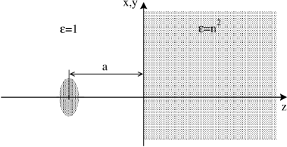
Figure 1: A sketch of the simplest system in cavity QED, consisting of a quantum object, e.g. an atom or an electron, that is located a distance $a$ away from a single reflecting wall. If the wall is perfectly reflecting then the electromagnetic field is excluded from the region $z>0$. A more realistic but still simple model is to describe the wall by a constant, frequency-independent refractive index $n$.

If one wanted to work in a gauge that resembles the radiation gauge, one ought to choose the gauge

$$\epsilon^{2}\frac{\partial\Phi}{\partial t}+\boldsymbol{\nabla}\cdot(\epsilon{\bf A})=0\;.$$

In this gauge Maxwell’s equations for the scalar potential $\Phi$ and the vector potential ${\bf A}$ read

$$\epsilon\frac{\partial^{2}\Phi}{\partial t^{2}}-\nabla^{2}\Phi=\frac{\rho}{\epsilon}+\frac{1}{\epsilon}(\boldsymbol{\nabla}\Phi)\cdot\boldsymbol{\nabla}\epsilon\ ,$$

$$\boldsymbol{\nabla}(\boldsymbol{\nabla}\cdot{\bf A})-\nabla^{2}{\bf A}+\epsilon\frac{\partial^{2}{\bf A}}{\partial t^{2}}-\epsilon\boldsymbol{\nabla}\left[\frac{1}{\epsilon^{2}}\boldsymbol{\nabla}\cdot(\epsilon{\bf A})\right]={\bf j}\ .$$

It is important that they separate and that for piecewise constant $\epsilon({\bf r})$ they differ from the standard wave equations for $\Phi$ and ${\bf A}$ only by surface terms. However, in the present paper we shall not pursue any calculations in this gauge but work in the generalized Coulomb gauge (1).

In Section II we calculate the full photon propagator in the presence of a non-dispersive dielectric half-space starting from the normal modes of the radiation field which we briefly discuss in Appendix A. In Section III we use this photon propagator to determine the self-energy of a free electron located outside and a distance $a$ away from the dielectric. In Section IV we do a careful asymptotic analysis of the expression for the self-energy for non-relativistic mean energies. In Section IV.4 we compare the results for the electron’s radiative self-energy in front of an imperfectly or of a perfectly reflecting surface and discuss the reasons for the disagreement between the calculation for a non-dispersive dielectric and for a “perfect reflector”. Section V summarizes our final results.

Throughout this paper we set $c=1=\hbar$ and use Heaviside-Lorentz units for electromagnetic quantities, $\epsilon_{0}=1=\mu_{0}$. Thus the fine structure constant is $e^{2}/4\pi\approx 1/137$.

II Calculation of the photon propagator

II.1 Wightman function

The Green’s functions in free quantum electrodynamics are vacuum expectation values of products of field operators. Let us first consider the Wightman functions bog

$$D^{\mu\,\nu\,-}(x,x^{\prime})=-i<0|A^{\mu}(x)A^{\nu}(x^{\prime})|0>\;.$$ (3)

Inserting the normal modes (61) and (64) into (3) and taking the vacuum expectations values of the bilinear products of photon annihilation and creation operators, we obtain

$$D^{\mu\,\nu\,-}(x,x^{\prime})=\sum_{\sigma}e^{\mu}_{\sigma}(\partial_{x})\,e^{\nu*}_{\sigma}(\partial_{x^{\prime}})\;g^{\sigma\sigma}\hskip 42.67912pt$$

$$\times\big{[}{{}^{L}D}_{\sigma}^{-}(x,x^{\prime})+{{}^{R}D}_{\sigma}^{-}(x,x^{\prime})\big{]}.$$ (4)

with

$${{}^{R}D}_{\sigma}^{-}(x,x^{\prime}) = i\int\frac{d^{2}k_{\parallel}}{(2\pi)^{3}}\int_{-\infty}^{0}dk^{d}_{z}\;\frac{1}{2\omega}\ e^{-i(\tilde{x}-\tilde{x}^{\prime})\tilde{k}}\Big{\{}\theta(-z)\theta(-z^{\prime})\big{[}e^{(ik_{z}z-ik_{z}^{*}z^{\prime})}T^{R}_{\sigma}{T^{R}_{\sigma}}^{*}\big{]}$$ (5)

$$+\theta(z)\theta(z^{\prime})\frac{1}{n^{2}}\big{[}e^{ik_{z}^{d}(z-z^{\prime})}+e^{ik^{d}_{z}(z+z^{\prime})}{R^{R}_{\sigma}(k)}^{*}+e^{-ik_{z}^{d}(z+z^{\prime})}R^{R}_{\sigma}(k)+e^{i(k_{z}^{d}(z-z^{\prime})}R^{R}_{\sigma}{R^{R}_{\sigma}}^{*}\big{]}$$

$$+\theta(-z)\theta(z^{\prime})\frac{1}{n}\big{[}e^{(ik_{z}z-ik_{z}^{d}z^{\prime})}T^{R}_{\sigma}+e^{ik_{z}z+ik_{z}^{d}z^{\prime})}T^{R}_{\sigma}{R^{R}_{\sigma}}^{*}\big{]}$$

$$+\theta(z)\theta(-z^{\prime})\frac{1}{n}\big{[}e^{(ik_{z}^{d}z-ik_{z}^{*}z^{\prime})}{T^{R}_{\sigma}}^{*}+e^{-ik_{z}^{d}z-ik_{z}^{*}z^{\prime})}R^{R}_{\sigma}{T^{R}_{\sigma}}^{*}\big{]}\Big{\}}\;,$$

and

$${{}^{L}D}_{\sigma}^{-}(x,x^{\prime}) = i\int\frac{d^{2}k_{\parallel}}{(2\pi)^{3}}\int_{0}^{\infty}dk_{z}\;\frac{1}{2\omega}\ e^{-i(\tilde{x}-\tilde{x}^{\prime})\tilde{k}}\Big{\{}\theta(z)\theta(z^{\prime})\frac{1}{n^{2}}e^{ik_{z}^{d}(z-z^{\prime})}T^{L}_{\sigma}{T^{L}_{\sigma}}^{*}$$ (6)

$$+\theta(-z)\theta(-z^{\prime})\big{[}e^{ik_{z}(z-z^{\prime})}+e^{ik_{z}(z+z^{\prime})}{R^{L}_{\sigma}(k)}^{*}+e^{-ik_{z}(z+z^{\prime})}R^{L}_{\sigma}(k)+e^{-ik_{z}(z-z^{\prime})}R^{L}_{\sigma}(k){R^{L}_{\sigma}(k)}^{*}\big{]}$$

$$+\theta(-z)\theta(z^{\prime})\frac{1}{n}\big{[}e^{(ik_{z}z-ik_{z}^{d}z^{\prime})}{T^{L}_{\sigma}}^{*}+e^{(-ik_{z}z-ik_{z}^{d}z^{\prime})}{T^{L}_{\sigma}}^{*}R^{L}_{\sigma}\big{]}$$

$$+\theta(z)\theta(-z^{\prime})\frac{1}{n}\big{[}e^{(ik_{z}^{d}z-ik_{z}z^{\prime})}T^{L}_{\sigma}+e^{(ik_{z}^{d}z+ik_{z}z^{\prime})}T^{L}_{\sigma}{R^{L}_{\sigma}}^{*}\big{]}\Big{\}}\;.$$

The notations for the wave vectors is as defined in Eq. (A), and in addition we have introduced the new variables $\tilde{k}=(k^{0},{\bf k}_{\parallel})$ and $\tilde{x}=(x^{0},{\bf x}_{\parallel})$ in 2+1 dimensional Minkowski space. The sum of ${{}^{L}D}_{\sigma}^{-}(x,x^{\prime})$ and ${{}^{R}D}_{\sigma}^{-}(x,x^{\prime})$ can be simplified by taking into account that the Fresnel coefficients are real functions of the wave vectors and by using various relations (66) and (67) between them and their products. We obtain two equivalent expressions:

$${{}^{L}D}_{\sigma}^{-}(x,x^{\prime})+{{}^{R}D}_{\sigma}^{-}(x,x^{\prime}) = i\int\frac{d^{2}k_{\parallel}}{(2\pi)^{3}}\frac{1}{2\omega}\ e^{-i(\tilde{x}-\tilde{x}^{\prime})\tilde{k}}\Bigg{\{}\theta(z)\theta(z^{\prime})\frac{1}{n^{2}}\int_{-\infty}^{\infty}dk_{z}^{d}\left[e^{ik_{z}^{d}(z-z^{\prime})}+e^{-ik_{z}^{d}(z+z^{\prime})}R^{R}_{\sigma}\right]$$ (7)

$$+\theta(-z)\theta(-z^{\prime})\left[\int_{-\infty}^{\infty}dk_{z}e^{ik_{z}(z-z^{\prime})}+\int_{-\infty}^{\infty}dk_{z}e^{-ik_{z}(z+z^{\prime})}R^{L}_{\sigma}+\int_{-\Gamma}^{0}dk_{z}^{d}e^{ik_{z}z-ik_{z}^{*}z^{\prime}}{T^{R}_{\sigma}}^{*}T^{R}_{\sigma}\right]$$

$$+\theta(-z)\theta(z^{\prime})\frac{1}{n}\int_{-\infty}^{\infty}dk_{z}^{d}e^{ik_{z}z-ik_{z}^{d}z^{\prime}}T^{R}_{\sigma}+\theta(z)\theta(-z^{\prime})\frac{1}{n}\int_{-\infty}^{\infty}dk_{z}e^{-ik_{z}z^{\prime}+ik_{z}^{d}z}{T^{R}_{\sigma}}^{*}\Bigg{\}}$$

and

$${{}^{L}D}_{\sigma}^{-}(x,x^{\prime})+{{}^{R}D}_{\sigma}^{-}(x,x^{\prime}) = i\int\frac{d^{2}k_{\parallel}}{(2\pi)^{3}}\frac{1}{2\omega}\ e^{-i(\tilde{x}-\tilde{x}^{\prime})\tilde{k}}\Bigg{\{}\theta(z)\theta(z^{\prime})\frac{1}{n^{2}}\int_{\infty}^{\infty}dk_{z}^{d}\left[e^{ik_{z}^{d}(z-z^{\prime})}+e^{-ik_{z}^{d}(z+z^{\prime})}R^{R}_{\sigma}\right]$$ (8)

$$+\theta(-z)\theta(-z^{\prime})\left[\int_{-\infty}^{\infty}dk_{z}e^{ik_{z}(z-z^{\prime})}+\int_{\mathcal{C}}dk_{z}e^{ik_{z}(z+z^{\prime})}R^{L}_{\sigma}\right]$$

$$+\theta(-z)\theta(z^{\prime})\frac{1}{n}\int_{-\infty}^{\infty}dk_{z}^{d}e^{ik_{z}z-k_{z}^{d}z^{\prime}}T^{R}_{\sigma}+\theta(z)\theta(-z^{\prime})\frac{1}{n}\int_{-\infty}^{\infty}dk_{z}e^{-ik_{z}z^{\prime}+ik_{z}^{d}z}{T^{R}_{\sigma}}^{*}\Bigg{\}},$$

with $\Gamma=((n^{2}-1)k_{\parallel}^{2})^{1/2}$. The difference between these two expressions is how the contributions from evanescent waves are included. In the first expression (7) they appear in the second line as a separate integral over $k_{z}^{d}$ from $-\Gamma$ to 0. In the second expression (8) they are included in the integration along the path $\mathcal{C}$ in the complex $k_{z}$ plane shown in Fig. 2: it runs along the real axis from $-\infty$ to $0$, then down the negative imaginary axis from $0$ to $-i\Gamma/n$ to the left of the square root cut, back up to the origin to the right of the cut, and then along the real axis from $0$ to $+\infty$. The cut is due to $k_{z}^{d}=(n^{2}k_{z}^{2}+(n^{2}-1)k_{\parallel}^{2})^{1/2}/n$ and extends from $k_{z}=+i\Gamma/n$ to $k_{z}=-i\Gamma/n$. The part of $\mathcal{C}$ that runs left and right of the cut is identical to the integral over $k_{z}^{d}$ in the second line of (7), i.e. it gives the contribution of the of the evanescent waves.

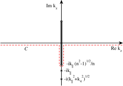
Figure 2: The integration path $\mathcal{C}$ in the complex $k_{z}$ plane.

This works because:

$$\left.R^{L}\right|_{k_{z}=-i\kappa,\,k_{z}^{d}=-K}-\left.R^{L}\right|_{k_{z}=-i\kappa,\,k_{z}^{d}=K}\hskip 42.67912pt$$

$$=\left.\frac{k_{z}}{k_{z}^{d}}n^{2}T^{R}{T^{R}}^{*}\right|_{k_{z}=-i\kappa,\,k_{z}^{d}=-K}\;.$$ (9)

Note that the $\omega=0$ singularity at $k_{z}=\pm ik_{\parallel}$ does not come into play if one chooses the cut of $\omega=(k_{z}^{2}+k_{\parallel}^{2})^{1/2}$ along $-i\infty\ldots-ik_{\parallel}$ and $ik_{\parallel}\ldots i\infty$.

II.2 Feynman propagator

For the calculation of radiative corrections we need the Feynman propagator, which can be reconstructed from the Wightman functions (II.1), (7) and (8) according to

$$D^{\mu\,\nu\,c}(x,x^{\prime}) = -i\langle 0|TA^{\mu}(x)A^{\nu}(x^{\prime})|0\rangle$$

$$= \theta(x^{0}-{x^{\prime}}^{0})\;D^{\mu\,\nu\,-}(x,x^{\prime})$$

$$+\theta({x^{\prime}}^{0}-x^{0})\;D^{\nu\,\mu\,-}(x^{\prime},x)$$

Thus $D^{\mu\,\nu\,c}(x,x^{\prime})$ can be written in the same way as the Wightman function in (II.1),

$$D^{\mu\,\nu\,c}(x,x^{\prime})=\sum_{\sigma}e^{\mu}_{\sigma}(\partial_{x})\,e^{\nu*}_{\sigma}(\partial_{x^{\prime}})\;g^{\sigma\sigma}\;D^{c}_{\sigma}(x,x^{\prime})\;.$$

The sum over the polarizations is gauge dependent. In Coulomb gauge the sum runs over $\sigma=TE,\ TM$ only. In covariant, i.e. Feynman gauge the two unphysical polarizations $G,\ C$ have to be included. Proceeding from the simplified expressions (7) and (8) for the Wightman functions, we obtain for the polarization component $\sigma$ of the Feynman propagator

$$D_{\sigma}^{c}(x,x^{\prime}) \!\!\!= \!\!\!-\!\int\!\frac{d^{3}\tilde{k}}{(2\pi)^{4}}\;e^{-i(\tilde{x}-\tilde{x}^{\prime})\tilde{k}}\left\{\;\theta(z)\theta(z^{\prime})\int_{-\infty}^{\infty}dk_{z}^{d}\left[e^{ik_{z}^{d}(z-z^{\prime})}+e^{-ik_{z}^{d}(z+z^{\prime})}R^{R}_{\sigma}\right]\frac{1}{n^{2}k_{0}^{2}-k_{p}^{2}-k_{z}^{d\,2}+i\epsilon}\right.$$

$$+\theta(-z)\theta(-z^{\prime})\left[\int_{-\infty}^{\infty}dk_{z}\;e^{ik_{z}(z-z^{\prime})}+\int_{\cal C}dk_{z}e^{ik_{z}(z+z^{\prime})}R^{L}_{\sigma}\right]\frac{1}{k^{2}+i\epsilon}$$

$$+\theta(-z)\theta(z^{\prime})\frac{1}{n}\int_{-\infty}^{\infty}dk_{z}^{d}\;e^{ik_{z}z-ik_{z}^{d}z^{\prime}}\;T^{R}_{\sigma}\;\frac{1}{k_{0}^{2}-(k_{p}^{2}+k_{z}^{d\,2})/n^{2}+i\epsilon}$$

$$\left.+\theta(z)\theta(-z^{\prime})\frac{1}{n}\int_{-\infty}^{\infty}dk_{z}^{d}\;e^{-ik_{z}z^{\prime}+ik_{z}^{d}z}\;T^{R*}_{\sigma}\;\frac{1}{k_{0}^{2}-(k_{p}^{2}+k_{z}^{d\,2})/n^{2}+i\epsilon}\right\}\;.$$

In an alternative formulation one can replace the second line of (II.2) by

$$\theta(-z)\theta(-z^{\prime})\left[\int_{-\infty}^{\infty}dk_{z}\;e^{ik_{z}(z-z^{\prime})}+\int_{-\infty}^{\infty}dk_{z}\;e^{ik_{z}(z+z^{\prime})}R^{L}_{\sigma}+\int_{-\Gamma}^{0}dk_{z}^{d}\;e^{ik_{z}z-ik^{*}_{z}z^{\prime}}T^{R*}_{\sigma}\;T^{R}_{\sigma}\right]\frac{1}{k^{2}+i\epsilon}$$ (11)

Note that the property $e^{\mu}_{\lambda}(\partial_{x})e^{\nu*}_{\lambda}(\partial_{x^{\prime}})=e^{\mu*}_{\lambda}(\partial_{x})e^{\nu}_{\lambda}(\partial_{x^{\prime}})$ follows directly from the definition (60) of the polarization vectors. Note also that $k_{0}$ in Eq. (II.2) is a free integration variable and is not fixed to $\omega$ as it was in the case of the Wightman functions (7) and (8).

The propagator differs from its equivalent in free space by not being translation invariant along $z$. However, it is still symmetric in its arguments, $D^{c}_{\sigma}(x,x^{\prime})=D^{c}_{\sigma}(x^{\prime},x)$. This is easily shown by a change of variables $k\rightarrow-k$. For real $k_{z}$ this is straightforward; for imaginary $k_{z}=-i\kappa$ (with $\kappa>0$) one needs the relation

$$T^{R}(k_{z}=-i\kappa,-k_{z}^{d})={T^{R*}(k_{z}=-i\kappa,k_{z}^{d})}\;,$$

for which one has to take care to stay on the same sheet in the complex plane.

The wave equations that the Feynman propagator satisfies are

$$(\partial_{x_{0}}^{2}-\Delta_{x})D^{c}_{\sigma}(x,x^{\prime}) = \delta^{(4)}(x-x^{\prime})\;,\qquad\mbox{for }z<0\;,$$

$$(n^{2}\partial_{x_{0}}^{2}-\Delta_{x})D^{c}_{\sigma}(x,x^{\prime}) = \delta^{(4)}(x-x^{\prime})\;,\qquad\mbox{for }z>0\;.$$

Checking the wave equation for example for $z<0$ leads to

$$(\partial_{x_{0}}^{2}-\Delta_{x})D_{\sigma}^{c}(x,x^{\prime}) \!\!\!= \!\!\!\theta(-z)\theta(-z^{\prime})\delta^{(4)}(x-x^{\prime})$$

$$+\int\frac{d^{3}\tilde{k}}{(2\pi)^{4}}e^{-i(\tilde{x}-\tilde{x}^{\prime})\tilde{k}}\left\{\theta(-z)\theta(-z^{\prime})\int_{-\infty}^{\infty}dk_{z}\;e^{ik_{z}(z-z^{\prime})}R^{L}_{\sigma}+\Theta(-z)\Theta(z^{\prime})\frac{1}{n}\int_{-\infty}^{\infty}dk_{z}^{d}\;e^{ik_{z}z-ik_{z}^{d}z^{\prime}}T^{R}_{\sigma}\right\}.$$

The second line should vanish, which it does — because the integration path can be closed in the lower $k_{z}$ plane as the Fresnel coefficients do not have poles there.

A direct check of the Feynman propagator is the reconstruction of the Wightman functions (7) and (8) by performing the $k_{0}$ integration. For $x_{0}>0$ the integration path can be closed in the lower half plane

$$\int_{-\infty}^{\infty}\frac{\exp(-ik_{0}x^{0})}{k_{0}^{2}+{\bf k}^{2}+i\epsilon}=-\frac{i}{2|{\bf k}|}\;\exp(-i|{\bf k}|x^{0})\;\theta(x_{0})\;,$$ (12)

and we thus reproduce (7) and (8) for $x_{0}-{x^{\prime}}_{0}>0$.

Next we consider two special cases. The simplest situation is the limit $n\rightarrow 1$, when there is no medium. Correspondingly all reflection coefficients $R$ tend to zero, the transmission coefficients $T$ approach one, and $\Gamma\rightarrow 0$, so that complex values do not appear in the integration over $k_{z}$. For all polarizations $\sigma$ the propagator components equal the massless scalar propagator

$$D_{\sigma}^{c}(x,x^{\prime})=-\int\frac{d^{4}k}{(2\pi)^{4}}e^{-i(x-x^{\prime})k}\frac{1}{k^{2}+i\epsilon}\;.$$ (13)

Thus, according to (A) our Feynman propagator (II.2) coincides in the limit $n\rightarrow 1$ with the standard free space propagators: either with the covariant propagator in Feynman gauge or with the propagator in Coulomb gauge, depending on which modes have been included in the sum over polarizations.

In the limit $n\rightarrow\infty$ only the left incident modes survive, so that, according to (A), the Wightman functions (II.1)and its components (7) simplify greatly.

$${D}_{\sigma}^{-}(x,x^{\prime})=i\int\frac{d^{2}k_{\parallel}}{(2\pi)^{3}}\int_{-\infty}^{\infty}\frac{dk_{z}}{2\omega}e^{-i(\tilde{x}-\tilde{x}^{\prime})\tilde{k}}\theta(-z)\theta(-z^{\prime})$$

$$\times\left[e^{ik_{z}(z-z^{\prime})}+e^{ik_{z}(z+z^{\prime})}{R^{L}_{\sigma}(k)}\right]\hskip 28.45274pt$$ (14)

with

$$R^{L}_{TE}=R^{L}_{C}=R^{L}_{G}=-1,R^{L}_{TM}=1.$$

A corresponding representation follows for the Feynman propagator.

Finally we need to establish the electrostatic Green function, which corresponds to the Coulomb interaction. One way to start is from the retarded Green function for the Coulomb mode $C$. The retarded propagator differs from the Feynman propagator (II.2) by the $i\epsilon$ prescription in the denominator, such that $i\epsilon\rightarrow i\epsilon k_{0}$. Since we are looking for a static Green’s function we need to calculate

$$G_{C}(\vec{x},\vec{x}^{\prime}) = \int dx^{0}\;D_{C}^{ret}(x,x^{\prime})$$

$$= \int\frac{d^{2}k_{\parallel}}{(2\pi)^{3}}e^{i({\bf x}_{\parallel}-{\bf x}^{\prime}_{\parallel})\cdot{\bf k}_{\parallel}}\frac{1}{{\bf k}^{2}}\left\{\theta(-z)\;\theta(-z^{\prime})\int_{-\infty}^{\infty}dk_{z}\left(e^{ik_{z}(z-z^{\prime})}+e^{ik_{z}(z+z^{\prime})}\frac{1-n^{2}}{1+n^{2}}\right)\right.$$

$$+\;\theta(z)\;\theta(z^{\prime})\int_{-\infty}^{\infty}dk_{z}\left(e^{ik_{z}(z-z^{\prime})}+e^{-ik_{z}(z+z^{\prime})}\frac{n^{2}-1}{n^{2}+1}\right)$$

$$\left.+\;\theta(-z)\;\theta(z^{\prime})\int_{-\infty}^{\infty}dk_{z}\;e^{ik_{z}(z-z^{\prime})}\frac{2n}{1+n^{2}}+\;\theta(z)\;\theta(-z^{\prime})\int_{-\infty}^{\infty}dk_{z}\;e^{ik_{z}(z-z^{\prime})}{\frac{2n}{1+n^{2}}}\right\}\;.$$

In our conventions $A^{0}(x)=\Phi^{0}(x)$ for $z<0$ and $A^{0}(x)=n\Phi^{0}(x)$ for $z>0$, so that we obtain for the electrostatic Green’s function

$$G_{\Phi}(x,x^{\prime}) = -i\langle 0|\Phi^{0}(x)\Phi^{0}(x^{\prime})|0\rangle$$

$$= \int\frac{d^{2}k_{\parallel}}{(2\pi)^{3}}\int_{-\infty}^{\infty}dk_{z}\;e^{i({\bf x}_{\parallel}-{\bf x}^{\prime}_{\parallel})\cdot{\bf k}_{\parallel}}\frac{1}{{\bf k}^{2}}\left\{\theta(-z)\;\theta(-z^{\prime})\left(e^{ik_{z}(z-z^{\prime})}+e^{ik_{z}(z+z^{\prime})}\frac{1-n^{2}}{1+n^{2}}\right)\right.$$

$$+\;\theta(z)\;\theta(z^{\prime})\;\frac{1}{n^{2}}\left(e^{ik_{z}(z-z^{\prime})}+e^{-ik_{z}(z+z^{\prime})}\frac{n^{2}-1}{n^{2}+1}\right)$$

$$\left.+\;\theta(-z)\;\theta(z^{\prime})\;e^{ik_{z}(z-z^{\prime})}\frac{2}{1+n^{2}}+\;\theta(z)\;\theta(-z^{\prime})\;e^{ik_{z}(z-z^{\prime})}{\frac{2}{1+n^{2}}}\right\}\;.$$

This result agrees with the classical electrostatic Green’s function, which can be derived easily, so that we have an additional check.

III The self-energy of the electron

The energy shift of the electron can be determined by considering the electron propagator and its radiative corrections due to the coupling to the photon field Weinberg . We start be considering the free electron propagator

$$S_{\alpha\beta}^{(0)}(x,y)=\langle 0|\,{\sf T}\,\psi_{\alpha}(x)\,\overline{\psi}_{\beta}(y)|0\rangle\;.$$ (17)

Using canonical quantization one can write the spinor

$$\psi_{\alpha}({\bf r},t)=\int\!\frac{d^{3}{\bf p}}{(2\pi)^{3/2}}\sqrt{\frac{m}{E}}\sum_{i=1,2}\left[b_{i,{\bf p}}u_{\alpha}^{(i)}({\bf p})e^{-iEt+i{\bf p}\cdot{\bf r}}\right.$$

$$\left.+d_{i,{\bf p}}^{\dagger}v_{\alpha}^{(i)}({\bf p})e^{iEt-i{\bf p}\cdot{\bf r}}\right]\;,\hskip 14.22636pt$$ (18)

where $b_{i,{\bf p}}$ annihilates an electron of helicity $i$ and momentum ${\bf p}$ and $d_{i,{\bf p}}^{\dagger}$ creates a positron of helicity $i$ and momentum ${\bf p}$. The particle eigenspinors $u_{\alpha}^{(i)}({\bf p})$ are solutions of the Dirac equation,

$$u^{(i)}({\bf p})=\sqrt{\frac{p^{0}+m}{2m}}\left(\begin{array}[]{c}\phi^{(i)}\\ \\ \displaystyle\frac{\boldsymbol{\sigma}\cdot{\bf p}}{p_{0}+m}\;\phi^{(i)}\end{array}\right),$$ (22)

with $\phi^{(i)}$ two orthogonal and normalized two-spinors. Thus the normalization of $u^{(i)}({\bf p})$ is

$$\overline{u}^{(i)}({\bf p})\,u^{(j)}({\bf p})=\delta_{ij}\,.$$

The antiparticle eigenspinors $v^{(i)}({\bf p})$ are similar to (22), except with upper and lower components interchanged and normalized to -1. Inserting the canonical expansion (18) and its conjugate into the expression for the propagator (17) and Fourier transforming to go from the time variable $(x_{0}-y_{0})$ to the energy $E$ one finds

$$S_{\alpha\beta}^{(0)}({\bf x},{\bf y},E)=-\int\!\frac{d^{3}{\bf p}}{(2\pi)^{3}}\frac{m}{E({\bf p})}\sum_{i=1,2}\frac{u^{(i)}({\bf p})\overline{u}^{(i)}({\bf p})}{E({\bf p})-E-i\epsilon}e^{i{\bf p}\cdot({\bf x}-{\bf y})}+\int\!\frac{d^{3}{\bf p}}{(2\pi)^{3}}\frac{m}{E({\bf p})}\sum_{i=1,2}\frac{\overline{v}^{(i)}({\bf p})v^{(i)}({\bf p})}{E({\bf p})+E-i\epsilon}e^{-i{\bf p}\cdot({\bf x}-{\bf y})}\;.\hskip 14.22636pt$$ (23)

This shows that the propagator has positive energy poles at the particle energies $E({\bf p})$ and negative energy poles at the antiparticle energies $-E({\bf p})$. Radiative corrections represent a perturbation and cause shifts in the particle and antiparticles eigenfunctions and in their energies. For small perturbations these shifts are small and expressions can be linearized in them. Linearizing the change of the propagator $\delta S=S-S^{(0)}$, one obtains a term that is linear in the energy shift and has a double pole at the particle or antiparticle energy,

$$\delta S_{\alpha\beta}^{(0)}({\bf x},{\bf y},E) \!\simeq \!\int\!\frac{d^{3}{\bf p}}{(2\pi)^{3}}\frac{m}{E({\bf p})}\sum_{i=1,2}\left\{\frac{u^{(i)}({\bf p})\overline{u}^{(i)}({\bf p})}{\left[E({\bf p})-E-i\epsilon\right]^{2}}e^{i{\bf p}\cdot({\bf x}-{\bf y})}-\frac{\overline{v}^{(i)}({\bf p})v^{(i)}({\bf p})}{\left[E({\bf p})+E-i\epsilon\right]^{2}}e^{-i{\bf p}\cdot({\bf x}-{\bf y})}\right\}\,\delta E({\bf p})$$ (24)

$$+\ \mbox{(other terms without double poles)}\;.$$

Further terms that are linear in the shifts of the particle and antiparticle eigenfunctions do not give rise to terms with double poles since the eigenfunctions appear only in the numerator of Eq. (23).

The energy shift $\delta E({\bf p})$ can now be determined by comparing the expression (24) to the change of the electron propagator as determined from standard Feynman perturbation theory. At one-loop level, i.e. to order $e^{2}$, the radiative correction to the propagator is

$$\delta S_{\alpha\beta}^{(0)}({\bf x},{\bf y},E)=\int d^{3}{\bf z}\int d^{3}{\bf z}^{\prime}\;S^{(0)}_{\alpha\gamma}({\bf x},{\bf z},E)\Sigma_{\gamma\kappa}({\bf z},{\bf z}^{\prime},E)$$

$$\times\ S^{(0)}_{\kappa\beta}({\bf z}^{\prime},{\bf y},E)\;,\hskip 14.22636pt$$ (25)

where $\Sigma_{\alpha\beta}({\bf x},{\bf x}^{\prime},E)$ is obtained from the standard electron self-energy

$$\Sigma_{\alpha\beta}(x,x^{\prime})=-ie^{2}\gamma^{\mu}_{\alpha\kappa}S^{(0)}_{\kappa\lambda}(x-x^{\prime})\gamma^{\nu}_{\lambda\beta}D^{c}_{\mu\nu}(x,x^{\prime})\;$$ (26)

by Fourier transformation from the time into the energy domain. The electron propagator $S^{(0)}(x-x^{\prime})$ is the same as in free space and thus translation invariant in all 4 directions, but the photon propagator $D^{c}_{\mu\nu}(x,x^{\prime})$ is affected by the presence of the dielectric medium and therefore not translation invariant in the $x_{3}$ direction. Substituting the representation (23) in terms of eigenfunctions into Eq. (25) one obtains

$$\delta S_{\alpha\beta}^{(0)}({\bf x},{\bf y},E)=\int d^{3}{\bf z}\int d^{3}{\bf z}^{\prime}\int\!\frac{d^{3}{\bf p}}{(2\pi)^{3}}\int\!\frac{d^{3}{\bf p}^{\prime}}{(2\pi)^{3}}\frac{m}{E({\bf p})}\frac{m}{E({\bf p}^{\prime})}\sum_{i=1,2}\sum_{j=1,2}\left[e^{i{\bf p}\cdot({\bf x}-{\bf z})+i{\bf p}^{\prime}\cdot({\bf z}^{\prime}-{\bf y})}\frac{u^{(i)}_{\alpha}({\bf p})\overline{u}^{(i)}_{\gamma}({\bf p})}{E({\bf p})-E-i\epsilon}\right.$$

$$\left.\times\ \Sigma_{\gamma\kappa}({\bf z},{\bf z}^{\prime},E)\frac{u^{(j)}_{\kappa}({\bf p}^{\prime})\overline{u}^{(j)}_{\beta}({\bf p}^{\prime})}{E({\bf p}^{\prime})-E-i\epsilon}+\ldots\right]$$ (27)

Further terms all contain antiparticle operators and at least one negative energy pole. Since we are interested in the energy shift of a particle rather than an antiparticle, we need to focus only on terms with two particle poles. For ${\bf p}={\bf p}^{\prime}$ Eq. (27) has the same double pole as Eq. (24), and thus a simple comparison of the coefficients of those double-pole terms should yield an expression for the energy shift $\delta E({\bf p})$ in (24). However, a mathematically clean comparison is possible only if one introduces a quantization volume $L^{3}$ with periodic boundary conditions so as to discretize the momentum ${\bf p}$. Then all integrals over momenta turn into sums according to the prescription

$$\int\!\frac{d^{3}{\bf p}}{(2\pi)^{3}}\longrightarrow\frac{1}{L^{3}}\sum_{\bf p}\;.$$

Only the term with ${\bf p}={\bf p}^{\prime}$ in the double sum over momenta in Eq. (27) gives rise to a double pole in the energy, and comparison with the double-pole term in Eq. (24) therefore yields

$$\delta E({\bf p})=\frac{1}{L^{3}}\int d^{3}{\bf z}\int d^{3}{\bf z}^{\prime}\frac{m}{E({\bf p})}\,e^{-i{\bf p}\cdot({\bf z}-{\bf z}^{\prime})}\,\overline{u}^{(i)}_{\gamma}({\bf p})$$

$$\times\ \Sigma_{\gamma\kappa}({\bf z},{\bf z}^{\prime},E)\,u^{(i)}_{\kappa}({\bf p})\;.$$ (28)

It is advantageous to work with the Fourier representation of $\Sigma$. Because of the lack of translation invariance in the $x_{3}$ direction, the Fourier transform of the self energy with respect to ${\bf x}-{\bf x}^{\prime}$ has a residual dependence on $x_{3}+x_{3}^{\prime}$,

$$\Sigma_{\alpha\beta}(x,x^{\prime})=\int\frac{d^{4}q}{(2\pi)^{4}}\;e^{-iq(x-x^{\prime})}\;\Sigma_{\alpha\beta}(q,x_{3}+x^{\prime}_{3})\;.$$ (29)

In a finite quantization volume the integral over $d^{3}{\bf q}$ again turns into a sum, and we can re-write Eq. (28) as

$$\delta E({\bf p})=\frac{1}{L^{6}}\int d^{3}{\bf z}\int d^{3}{\bf z}^{\prime}\sum_{\bf q}\frac{m}{E({\bf p})}\,e^{i({\bf q}-{\bf p})\cdot({\bf z}-{\bf z}^{\prime})}\,\overline{u}^{(i)}_{\gamma}({\bf p})$$

$$\times\ \Sigma_{\gamma\kappa}(q,z_{3}+z_{3}^{\prime})\,u^{(i)}_{\kappa}({\bf p})\;.\hskip 14.22636pt$$ (30)

Since we want to work out the energy shift of a particle as a function of its distance from the dielectric, we need to form localized wave packets in the $x_{3}$ direction — so that the concept of a certain distance between the electron and the surface of the dielectric at all makes sense. If the centre of the packet is at $x_{3}=-a$ (see Fig. 1) then we can approximate $z_{3}+z_{3}^{\prime}\simeq-2a$ and carry out the ${\bf z}$ and ${\bf z}^{\prime}$ integrations in (30). The result simplifies to

$$\delta E({\bf p})=\frac{m}{E({\bf p})}\,\overline{u}^{(i)}_{\gamma}({\bf p})\,\Sigma_{\gamma\kappa}(p,-2a)\,u^{(i)}_{\kappa}({\bf p})\;.$$ (31)

Note that, while $\Sigma(q,x_{3}+x^{\prime}_{3})$ in Eq. (29) is in general off shell, it is on the mass shell in Eqs. (30) and (31) because $q$ and $p$ are on shell.

Further we need to remark that in Coulomb gauge the energy shift is not wholly due to the radiative self energy (26): we have to add to (31) the electrostatic energy

$$\delta E_{\mbox{\scriptsize Coulomb}}=\frac{e^{2}}{2}\int d^{3}x\int d^{3}x^{\prime}\;\langle:\overline{\psi}(x)\gamma^{0}\psi(x):$$

$$\times\ \overline{G}_{\Phi}(x,x^{\prime})\;:\overline{\psi}(x^{\prime})\gamma^{0}\psi(x^{\prime}):\rangle\,\,,$$ (32)

where $\overline{G}_{\Phi}$ is the part of the electrostatic Green’s function (II.2) that depends on the presence of the dielectric. The electrostatic shift is easy to evaluate, which we shall do in Section IV.5.

We are interested in the self-energy corrections for an electron located well outside the dielectric. Because of the electron’s localization its direct interaction with the dielectric medium is completely negligible, i.e. there is no wave-function overlap between the electron and the microscopic constituents of the dielectric. That is why, for $x_{3}<0$ and $x^{\prime}_{3}<0$ we can work with the standard free electron propagator,

$$S^{(0)}(x-x^{\prime}) = (i\gamma^{\mu}\partial_{x^{\mu}}+m)D^{c}_{m}(x-x^{\prime})\;,$$ (33)

$$D^{c}_{m}(x-x^{\prime}) = -\int\frac{d^{4}q}{(2\pi)^{4}}\,e^{-iq(x-x^{\prime})}\,\frac{1}{q^{2}-m^{2}+i\epsilon}\;.$$

The impact of the dielectric medium onto the self-energy of the electron is consequently just due to the electromagnetic interaction, i.e. due to the fact that the photon propagator (II.2) depends on the presence and electromagnetic properties of the medium. Since we are interested only in the energy shift due to the presence of the dielectric, we split the photon propagator into the free photon propagator and a medium-dependent part,

$$D^{c}(x,x^{\prime})=D^{c}_{(0)}(x,x^{\prime})+\overline{D}(x,x^{\prime})\;,$$

and take only the medium-dependent part $\overline{D}(x,x^{\prime})$ for calculating the self-energy (26) and the energy shift (31). This also means that we do not have to deal with regularization and renormalization; these have been done in the free part of the photon field, and we work with already renormalized quantities. All medium-dependent corrections will then automatically be finite.

From (II.2) we see that for $z<0$ and $z^{\prime}<0$, i.e. outside the dielectric, the medium-dependent part of the photon propagator is

$$\overline{D}^{\mu\,\nu\,c}(x,x^{\prime})|_{z,z^{\prime}<0}=-\sum_{\sigma}e^{\mu}_{\sigma}(\partial_{x})\,e^{\nu*}_{\sigma}(\partial_{x^{\prime}})\,g^{\sigma\sigma}\overline{D}^{c}_{\sigma}(x,x^{\prime})$$

$$\overline{D}^{c}_{\sigma}(x,x^{\prime})=\int\!\frac{d^{3}\tilde{k}}{(2\pi)^{4}}\int_{\cal C}dk_{z}\,e^{-i\tilde{k}(\tilde{x}-\tilde{x}^{\prime})+ik_{z}(z+z^{\prime})}R^{L}_{\sigma}\frac{1}{k^{2}+i\epsilon}\;.$$

(34)

The derivatives of the polarization vectors (60) act on a plane wave and its reflection. We obtain

$$e^{\mu}_{\sigma}(\partial_{x})\,e^{\nu*}_{\sigma}(\partial_{x^{\prime}})\;g^{\sigma\sigma}\;e^{-i\tilde{k}(\tilde{x}-\tilde{x}^{\prime})+ik_{z}(z+z^{\prime})}$$

$$=g^{\mu\nu}_{\sigma}(k)\;e^{-i\tilde{k}(\tilde{x}-\tilde{x}^{\prime})+ik_{z}(z+z^{\prime})}$$

with

$$g^{\mu\,\nu}_{TE}(k) = g^{m\,n}-\frac{k_{m}k_{n}}{-k_{\parallel}^{2}}=-\left(\delta_{m\,n}-\frac{k_{m}k_{n}}{k_{\parallel}^{2}}\right),$$

$$g^{\mu\,\nu}_{TM}(k) = \left\{g^{mn}=\frac{k_{m}k_{n}k_{z}^{2}}{{\bf k}^{2}k_{\parallel}^{2}},\ g^{m3}=\frac{k_{m}k_{z}}{{\bf k}^{2}},\right.$$ (35)

$$\left.\hskip 8.53581ptg^{3m}=-\frac{k_{z}^{*}k_{m}}{{\bf k}^{2}},\ g^{33}=-\frac{k_{\parallel}^{2}}{{\bf k}^{2}}\right\}$$

$$g^{\mu\nu}_{C}(k) = g^{00}\,,$$

$$g^{\mu\nu}_{G}(k) = \left\{g^{mn}=-\frac{k_{m}k_{n}}{{\bf k}^{2}},\ g^{33}=\frac{k_{z}^{2}}{{\bf k}^{2}},\right.$$

$$\left.\hskip 8.53581ptg^{m3}=\frac{k_{z}k_{m}}{{\bf k}^{2}}=-g^{3m}\right\}$$

where $m,n=1,2$. For evanescent waves one has $k_{z}=-i\kappa$, $k_{z}^{2}=-\kappa^{2}$, and ${\bf k}^{2}=k_{\parallel}^{2}-\kappa^{2}$.

Inserting the electron propagator (33) and the photon propagator (34) into the expression for the self energy (26), we have to multiply several $\gamma$ matrices. Using

$$\gamma^{\mu}\gamma^{\lambda}\gamma^{\nu} \!\!= \!\!s^{\alpha\mu\lambda\nu}\gamma_{\alpha}-i\epsilon^{\alpha\mu\lambda\nu}\gamma_{5}\gamma_{\alpha},\hskip 8.53581pt\epsilon_{0123}=+1,$$

$$s^{\alpha\mu\lambda\nu} \!\!= \!\!g^{\alpha\mu}g^{\lambda\nu}+g^{\alpha\nu}g^{\lambda\mu}-g^{\alpha\lambda}g^{\nu\mu}\;,$$ (36)

we encounter the following $\gamma$ valued invariants

$$I_{1}^{\sigma} \!\!= \!\!mg^{\mu\nu}g_{\mu\nu}^{\sigma}\,,\ \ \ \ I_{15}^{\sigma}=\frac{m}{2}[\gamma^{\mu},\gamma^{\nu}]g_{\mu\nu}^{\sigma}\,,$$

$$I_{25}^{\sigma} \!\!= \!\!\epsilon^{\alpha\mu\lambda\nu}\gamma_{5}\gamma_{\alpha}g_{\mu\nu}^{\sigma}q_{\lambda}\,,$$

$$I_{2}^{\sigma} \!\!= \!\!s^{\alpha\mu\lambda\nu}\gamma_{\alpha}g_{\mu\nu}^{\sigma}q_{\lambda}=g^{\mu\nu}_{\sigma}\gamma_{\mu}q_{\nu}+g^{\nu\mu}_{\sigma}\gamma_{\mu}q_{\nu}-(\gamma q)I_{1}^{\sigma}/m\,,$$

with $q$ being the Fourier variable in the electron propagator (33) and $g_{\mu\nu}^{\sigma}$ having the $k$ dependence as in (35). In terms of those the distance-dependent part of the self energy is

$$\Sigma=\sum_{\sigma}\Sigma^{\sigma}\ ,\hskip 14.22636pt\Sigma^{\sigma}=\left[\Sigma^{\sigma}_{1}+\Sigma^{\sigma}_{15}+\Sigma^{\sigma}_{2}+\Sigma^{\sigma}_{25}\right]$$ (37)

with

$$\Sigma^{\sigma}_{\theta}(x,x^{\prime}) \!\!= \!\!-ie^{2}\!\int\frac{d^{4}q}{(2\pi)^{4}}\int\frac{d^{3}\tilde{k}}{(2\pi)^{4}}\int_{C}dk_{z}\frac{e^{-iq(x-x^{\prime})}}{q^{2}-m^{2}+i\epsilon}$$ (38)

$$\times\ I_{\theta}^{\sigma}(q,k)\frac{e^{-i\tilde{k}(\tilde{x}-\tilde{x}^{\prime})+ik_{z}(z+z^{\prime})}}{k^{2}+i\epsilon}R^{L}_{\sigma}\;.$$

In the same way as for the total self energy in Eq. (29) we perform a Fourier transformation for the components in the sum (37), which again retain a dependence on $z+z^{\prime}$ due to the broken translation invariance in the $z$ direction,

$$\Sigma^{\sigma}_{\theta}(x,x^{\prime})=\int\frac{d^{4}p}{(2\pi)^{4}}\;e^{-ip(x-x^{\prime})}\,\Sigma^{\sigma}_{\theta}(p,z+z^{\prime})\;.$$

Making the variable replacements $\tilde{q}=\tilde{p}-\tilde{k}$, ${q}_{z}=p_{z}$ in Eq. (38) we obtain

$$\Sigma^{\sigma}_{\theta}(p,z+z^{\prime})=-ie^{2}\int\frac{d^{3}\tilde{k}}{(2\pi)^{4}}\int_{C}dk_{z}\;\frac{1}{(\tilde{p}-\tilde{k})^{2}-p_{z}^{2}-m^{2}+i\epsilon}\;I_{\theta}^{\sigma}(\tilde{p}-\tilde{k},p_{z},k)\;\frac{e^{ik_{z}(z+z^{\prime})}}{\tilde{k}^{2}-k_{z}^{2}+i\epsilon}R^{L}_{\sigma}\;.$$ (39)

This expression looks much simpler than it is to evaluate. The loss of translation invariance perpendicular to the surface of dielectric is one source of complications, and the interference of incident and reflected waves is another. In order to evaluate the self energy components (39) we need the explicit expressions for the invariants $I^{\sigma}_{\theta}$, which depend on the mode $\sigma$. For the two physical modes we find

$$I_{1}^{TE} \!\!= \!\!m\,,\ \ I_{15}^{TE}=0\,,\ \ I_{25}^{TE}=0\,,$$

$$I_{2}^{TE} \!\!= \!\!-2\left[\boldsymbol{\gamma}_{\parallel}\cdot({\bf p}_{\parallel}-{\bf k}_{\parallel})-\boldsymbol{\gamma}_{\parallel}\cdot{\bf k}_{\parallel}\frac{{\bf k}_{\parallel}\cdot({\bf p}_{\parallel}-{\bf k}_{\parallel})}{k_{\parallel}^{2}}\right]+\boldsymbol{\gamma}_{\parallel}\cdot({\bf p}_{\parallel}-{\bf k}_{\parallel})+\gamma_{3}p_{z}-\gamma_{0}(p_{0}-k_{0})\,,$$ (40)

$$I_{1}^{TM} \!\!= \!\!m\left(1-2\frac{k_{z}^{2}}{{\bf k}^{2}}\right)\,,\ \ I_{15}^{TM}=-m\frac{1}{{\bf k}^{2}}\,[\gamma^{3},\gamma^{n}]\,k_{z}k^{n}\,,\ \ I_{25}^{TM}=2\epsilon^{\alpha m\lambda 3}\gamma_{5}\gamma_{\alpha}(p_{\lambda}-k_{\lambda})\frac{k_{m}k_{z}}{{\bf k}^{2}},$$

$$I_{2}^{TM} \!\!= \!\!2\left\{\frac{(\boldsymbol{\gamma}_{\parallel}\cdot{\bf k}_{\parallel})\left[{\bf k}_{\parallel}\cdot({\bf p}_{\parallel}-{\bf k}_{\parallel})\right]}{k_{\parallel}^{2}{\bf k}^{2}}k_{z}^{2}-p_{z}\gamma_{3}\frac{k_{\parallel}^{2}}{{\bf k}^{2}}\right\}+\left[\boldsymbol{\gamma}_{\parallel}\cdot({\bf p}_{\parallel}-{\bf k}_{\parallel})+\gamma_{3}p_{z}-\gamma_{0}(p_{0}-k_{0})\right]\left(1-2\frac{k_{z}^{2}}{{\bf k}^{2}}\right).$$ (41)

IV Asymptotic analysis of the self-energy

IV.1 General approach and approximations

Our aim is to determine the energy shift of an electron that is localized in $z$-direction. The shift will depend on the distance $a$ of the electron from the surface of the dielectric, and without localization the notion of this distance would not make sense. Physically the localization could be realized be sending a tightly focussed beam parallel to the surface or by confining the electron by means of magnetic and/or electric fields. So, we will in fact not be working directly with momentum eigenstates (22) but use them to form with wave packets that peak at $z=a$ and whose average momentum in $z$ direction is $p_{z}$. The wave packet may move as a whole, which is why we have not approximated ${\bf z}-{\bf z}^{\prime}$ in Eq. (30); but we shall assume the electromagnetic field to be the same across the packet, which corresponds to the dipole approximation in atomic physics, and which is why we have set $z_{3}+z_{3}^{\prime}\simeq-2a$ in Eq. (31).

The extent of the wave packet must be small compared with the distance $a$ from the surface, but otherwise the details of the wave packet are not relevant. This implies $am\gg 1$, i.e. that the distance $a$ must be very much larger than the Compton wavelength $\lambdabar_{C}=\hbar/(mc)$. Thus, we shall aim for an expansion in $1/(ap_{0})$.

In order to proceed with the calculation of the self energy (39), we want to perform a Wick rotation $k_{0}=ik_{4}$. By design, the poles of the photon propagator lie in the right position for this. However, the poles of the term that originates from the electron propagator may interfere; they lie at $k_{0}=p_{0}\pm[\sqrt{({\bf p}_{\parallel}-{\bf k}_{\parallel})^{2}+p_{z}^{2}+m^{2}}-i\epsilon]$. There is no problem if they come to lie in the 2nd and 4th quadrant of the complex $k_{0}$ plane, but for $2{\bf p}_{\parallel}\cdot{\bf k}_{\parallel}>{\bf k}_{\parallel}^{2}$, one of the poles lies in the 1st rather than the 2nd quadrant, if we take $p$ to be on-shell, and a pole in the 1st quadrant interferes with the Wick rotation. There are several ways of dealing with this problem. One could work with a strongly deformed integration path and then carry along the separate contribution from the pole; or one could go off-shell to move the pole out of the 1st quadrant and then do an analytic continuation to a result for on-shell $p$; or one could avoid the problem altogether by approximating $p_{\parallel}\approx 0$ in the denominator of (39). We have decided on the last approach because it is straightforward and we are not interested in ultrarelativistic motion of the electron.

Thus we set $p_{\parallel}=0$ in the denominator of (39) but leave $p_{\parallel}$ untouched elsewhere, i.e. retain it in $I^{\sigma}_{\theta}$ (40) and (41). Then we can perform the Wick rotation $k_{0}=ik_{4}$ without problems and obtain

$$\Sigma^{\sigma}_{\theta}(p,z+z^{\prime})=e^{2}\int\frac{d^{2}k_{\parallel}}{(2\pi)^{4}}\int_{-\infty}^{\infty}dk_{4}\frac{1}{k_{4}^{2}+2ip_{0}k_{4}+{\bf k}_{\parallel}^{2}}$$

$$\times\int_{C}dk_{z}\;I_{\theta}^{\sigma}\frac{e^{ik_{z}(z+z^{\prime})}}{k_{4}^{2}+{\bf k}_{\parallel}^{2}+k_{z}^{2}}R^{L}_{\sigma}\;.$$

The integration over the three dimensional (Euclidean) space $({\bf k}_{\parallel},k_{4})$ can be carried out in spherical polar coordinates by defining $k_{4}=\rho\cos\vartheta,k_{x}=\rho\sin\vartheta\cos\varphi,k_{y}=\rho\sin\vartheta\sin\varphi$. We find

$$\Sigma^{\sigma}_{\theta}(p,z+z^{\prime})=\frac{e^{2}}{(2\pi)^{3}}\int_{0}^{\infty}d\rho\int_{-1}^{1}d(\cos\vartheta)\frac{\rho^{2}}{\rho^{2}+2ip_{0}\rho\cos\vartheta}$$

$$\times\int_{C}dk_{z}\;\frac{e^{ik_{z}(z+z^{\prime})}}{\rho^{2}+k_{z}^{2}}R^{L}_{\sigma}\ \frac{1}{2\pi}\int_{0}^{2\pi}\!\!d\varphi\;I_{\theta}^{\sigma}\;.\hskip 14.22636pt$$ (42)

The only $\varphi$ dependence is in the invariants $I_{\theta}^{\sigma}$; carrying out the integration and using the fact that $p$ is on-shell, one gets

$$\frac{1}{2\pi}\int_{0}^{2\pi}d\varphi\;\left(I_{1}^{TE}+I_{2}^{TE}\right) \!\!= \!\!\gamma_{0}i\rho\cos\vartheta-\boldsymbol{\gamma}_{\parallel}\cdot{\bf p}_{\parallel}\;,$$

$$\frac{1}{2\pi}\int_{0}^{2\pi}d\varphi\;\left(I_{1}^{TM}+I_{2}^{TM}\right) \!\!= \!\!-\gamma_{0}i\rho\cos\vartheta+\boldsymbol{\gamma}_{\parallel}\cdot{\bf p}_{\parallel}$$

$$+\frac{{\bf k}_{\parallel}^{2}}{{\bf k}^{2}}\left(2\gamma_{0}i\rho\cos\vartheta-2\gamma_{3}p_{z}-\boldsymbol{\gamma}_{\parallel}\cdot{\bf p}_{\parallel}\right)\,,$$

$$\int_{0}^{2\pi}d\varphi\;I_{15}^{TM}=0\;, \int_{0}^{2\pi}d\varphi\;I_{25}^{TM}=0\;.$$

The next step in the evaluation of Eq. (42) is to carry out the integration over $k_{z}$ by means of contour integration. The remaining two-dimensional integral over $\rho$ and $\cos\vartheta$ can then be calculated asymptotically for $|z+z^{\prime}|$ very much larger than the Compton wavelength. Since the technical details differ between the $TE$ and $TM$ polarizations, we consider their contributions one after the other. While the calculation to follow is perfectly general for all values of $z$ and $z^{\prime}$, provided $|z+z^{\prime}|p_{0}\gg 1$, we now simplify the notation and set $z+z^{\prime}=-2a$, as this is the value at which we need to evaluate the self energy in Eq. (31) for the radiative shift.

IV.2 TE contributions to the self energy

For the TE polarization the integrand of (42) has only one pole in the lower $k_{z}$ plane, and that is at $k_{z}=-i\rho=-i({\bf k}_{\parallel}^{2}+k_{4}^{2})^{1/2}$ (cf. Fig. 2). The $k_{z}$ integration can thus easily be carried out by deforming the contour ${\cal C}$ and evaluating the residue at $-i\rho$. We emphasize that when evaluating the reflection coefficient $R^{L}_{TE}$, Eq. (A), at this point, one must take great care that the branch cut of the square root in $k_{z}^{d}$ is indeed taken to run as shown in Fig. 2. Renaming $\cos\vartheta=t$, we can write the result of the contour integration as

$$\Sigma^{TE} \!\!= \!\!\frac{e^{2}}{8\pi^{2}}\int_{0}^{\infty}\!\!d\rho\int_{-1}^{1}\!dt\;\frac{\gamma_{0}i\rho t-\boldsymbol{\gamma}_{\parallel}\cdot{\bf p}_{\parallel}}{\rho+2ip_{0}t}R^{L}_{TE}(t)\;e^{-2a\rho}$$

$$\!\!= \!\!\frac{e^{2}}{4\pi^{2}}\int_{0}^{\infty}\!\!d\rho\int_{0}^{1}\!dt\;\rho\;\frac{2\gamma_{0}p_{0}t^{2}-\boldsymbol{\gamma}_{\parallel}\cdot{\bf p}_{\parallel}}{\rho^{2}+4p_{0}^{2}t^{2}}R^{L}_{TE}(t)\;e^{-2a\rho}$$

with

$$R^{L}_{TE}(t)=\frac{1-\sqrt{(n^{2}-1)t^{2}+1}}{1+\sqrt{(n^{2}-1)t^{2}+1}}\;.$$ (43)

Next we scale the integration variable $\rho=2p_{0}t\xi$. In terms of the new variable $\xi$ the integral reads

$$\Sigma^{TE}=\frac{e^{2}}{4\pi^{2}}\int_{0}^{\infty}d\xi\int_{0}^{1}dt\;\xi\;\frac{2\gamma_{0}p_{0}t^{2}-\boldsymbol{\gamma}_{\parallel}\cdot{\bf p}_{\parallel}}{\xi^{2}+1}$$

$$\times\;R^{L}_{TE}(t)\;e^{-4p_{0}at\xi}\;.$$ (44)

This integral can be evaluated asymptotically for large values of $p_{0}a$. A standard method of obtaining an asymptotic expansion for integrals with an exponentially damped integrand is repeated integration by parts. However, in two-dimensional integrals like the one above, this method generally fails because integration by parts in one variable generates inverse powers of the other variable and the resulting integral diverges at the lower limit. For a general discussion of this problem and its remedy, we refer the reader to Ref. siklos . Here we observe that $R^{L}_{TE}(t)$ and hence the integrand of (44) actually behave as $O(t^{2})$ for $t\rightarrow 0$. Thus we can integrate by parts in the $\xi$ integral twice without jeopardizing the convergence of the $t$ integral. In this way we find to leading order in $1/(p_{0}a)$

$$\Sigma^{TE}\approx\frac{e^{2}}{4\pi^{2}}\frac{1}{(4p_{0}a)^{2}}\int_{0}^{1}dt\;\frac{2\gamma_{0}p_{0}t^{2}-\boldsymbol{\gamma}_{\parallel}\cdot{\bf p}_{\parallel}}{t^{2}}R^{L}_{TE}(t)\;.$$ (45)

The $t$ integral in this expression is elementary.

IV.3 TM contributions to the self energy

The TM polarization is more difficult to deal with, since the invariants $I_{\theta}^{TM}$ introduce a factor $1/{\bf k}^{2}$ into the integrand of (42), which leads to an additional pole in the lower $k_{z}$ plane at $k_{z}=-i\rho\sin\vartheta=-ik_{\parallel}$ (cf. Fig. 2). Thus, closing the contour in the lower $k_{z}$ plane picks up two residues, one at $-i\rho$ and one at $-i\rho\sin\vartheta$. The result is

$$\Sigma^{TM} \!\!= \!\!\frac{e^{2}}{8\pi^{2}}\int_{0}^{\infty}\!\!d\rho\int_{-1}^{1}\!dt\;\frac{1}{\rho+2ip_{0}t}\left\{\left[\boldsymbol{\gamma}_{\parallel}\cdot{\bf p}_{\parallel}-\gamma_{0}i\rho t+\frac{1-t^{2}}{t^{2}}\left(\boldsymbol{\gamma}_{\parallel}\cdot{\bf p}_{\parallel}-2\gamma_{0}i\rho t+2\gamma_{3}p_{z}\right)\right]R^{L}_{TM}(t)\;e^{-2a\rho}\right.$$ (46)

$$\hskip 170.71652pt\left.-\frac{\sqrt{1-t^{2}}}{t^{2}}\left(\boldsymbol{\gamma}_{\parallel}\cdot{\bf p}_{\parallel}-2\gamma_{0}i\rho t+2\gamma_{3}p_{z}\right)R^{L}_{TM}(0)\;e^{-2a\rho\sqrt{1-t^{2}}}\right\}$$

$$\!\!= \!\!\frac{e^{2}}{4\pi^{2}}\int_{0}^{\infty}\!\!d\rho\int_{0}^{1}\!dt\;\frac{\rho}{\rho^{2}+4p_{0}^{2}t^{2}}\left\{\left[\frac{1}{t^{2}}\boldsymbol{\gamma}_{\parallel}\cdot{\bf p}_{\parallel}-2\gamma_{0}p_{0}\left(2-t^{2}\right)+\frac{1-t^{2}}{t^{2}}2\gamma_{3}p_{z}\right]R^{L}_{TM}(t)\;e^{-2a\rho}\right.$$

$$\hskip 170.71652pt\left.-\frac{\sqrt{1-t^{2}}}{t^{2}}\left(\boldsymbol{\gamma}_{\parallel}\cdot{\bf p}_{\parallel}-4\gamma_{0}p_{0}t^{2}+2\gamma_{3}p_{z}\right)R^{L}_{TM}(0)\;e^{-2a\rho\sqrt{1-t^{2}}}\right\}$$

where we have again renamed $\cos\vartheta=t$ and abbreviated

$$R^{L}_{TM}(t)=\frac{n^{2}-\sqrt{(n^{2}-1)t^{2}+1}}{n^{2}+\sqrt{(n^{2}-1)t^{2}+1}}\;.$$

As before, we are interested in an asymptotic result for $\Sigma^{TM}$ for large values of $p_{0}a$. To be able to do asymptotic analysis one needs to separate the terms with different arguments in the exponential. However, doing this simple-mindedly leads to two divergent integrals because their integrands each behave as $O(t^{-2})$ for $t\rightarrow 0$. That is why we add and subtract the same term and subdivide the integral as follows,

$$\Sigma^{TM}=\Sigma^{TM}_{A}+\Sigma^{TM}_{B}+\Sigma^{TM}_{C}+\Sigma^{TM}_{D}\;,$$ (47)

with

$$\Sigma^{TM}_{A} \!\!= \!\!\frac{e^{2}}{4\pi^{2}}\int_{0}^{\infty}\!\!d\xi\int_{0}^{1}\!dt\;\frac{\xi}{\xi^{2}+1}\left[2\gamma_{0}p_{0}\left(t^{2}-2\right)-2\gamma_{3}p_{z}\right]R^{L}_{TM}(t)\;e^{-4p_{0}at\xi}$$

$$\Sigma^{TM}_{B} \!\!= \!\!\frac{e^{2}}{4\pi^{2}}\left(2\gamma_{3}p_{z}+\boldsymbol{\gamma}_{\parallel}\cdot{\bf p}_{\parallel}\right)\int_{0}^{\infty}\!\!d\xi\int_{0}^{1}\!dt\;\frac{\xi}{\xi^{2}+1}\frac{1}{t^{2}}\left[R^{L}_{TM}(t)-R^{L}_{TM}(0)\right]\;e^{-4p_{0}at\xi}$$

$$\Sigma^{TM}_{C} \!\!= \!\!\frac{e^{2}}{4\pi^{2}}\left(2\gamma_{3}p_{z}+\boldsymbol{\gamma}_{\parallel}\cdot{\bf p}_{\parallel}\right)R^{L}_{TM}(0)\int_{0}^{\infty}\!\!d\xi\int_{0}^{1}\!dt\;\frac{\xi}{\xi^{2}+1}\frac{1}{t^{2}}\left(e^{-4p_{0}at\xi}-\sqrt{1-t^{2}}e^{-4p_{0}at\sqrt{1-t^{2}}\xi}\right)$$

$$\Sigma^{TM}_{D} \!\!= \!\!\frac{e^{2}}{4\pi^{2}}4\gamma_{0}p_{0}R^{L}_{TM}(0)\int_{0}^{\infty}\!\!d\xi\int_{0}^{1}\!dt\;\frac{\xi}{\xi^{2}+1}\sqrt{1-t^{2}}\;e^{-4p_{0}at\sqrt{1-t^{2}}\xi}$$

where we have again rescaled $\rho=2p_{0}t\xi$.

We do the asymptotic analysis of these integrals one by one, starting with $\Sigma^{TM}_{A}$. In order to get an asymptotic expansion for large $p_{0}a$, one would try to integrate by parts. However, The integrand of $\Sigma^{TM}_{A}$ behaves as $O(1)$ for $t\rightarrow 0$, and thus the factor $1/t$ that one gets through integrating by parts in the $\xi$ integral would destroy the convergence at $t=0$. Adapting the general method of obtaining an asymptotic expansion of such two-dimensional integrals siklos , we add and subtract the problematic point at $t=0$ and write

$$\Sigma^{TM}_{A} \!\!= \!\!-\frac{e^{2}}{4\pi^{2}}\int_{0}^{\infty}\!\!d\xi\int_{0}^{1}\!dt\;\frac{\xi}{\xi^{2}+1}\left(4\gamma_{0}p_{0}+2\gamma_{3}p_{z}\right)R^{L}_{TM}(0)\;e^{-4p_{0}at\xi}$$

$$+\frac{e^{2}}{4\pi^{2}}\int_{0}^{\infty}\!\!d\xi\int_{0}^{1}\!dt\;\frac{\xi}{\xi^{2}+1}\left\{\left[2\gamma_{0}p_{0}\left(t^{2}-2\right)-2\gamma_{3}p_{z}\right]R^{L}_{TM}(t)+\left(4\gamma_{0}p_{0}+2\gamma_{3}p_{z}\right)R^{L}_{TM}(0)\right\}e^{-4p_{0}at\xi}$$

The first of the integrals is easy to calculate; the $t$ integral is immediate, and the remaining integral over $\xi$ is a well known combination of sine and cosine integrals as . The integrand of the second integral now behaves as $O(t^{2})$ for $t\rightarrow 0$, and we can thus integrate by parts twice without getting convergence problems at $t=0$. In this way we find to order $1/(p_{0}a)^{2})$

$$\Sigma^{TM}_{A}\approx-\frac{e^{2}}{8\pi^{2}p_{0}a}\left(2\gamma_{0}p_{0}+\gamma_{3}p_{z}\right)R^{L}_{TM}(0)\left(\frac{\pi}{2}-\frac{1}{4p_{0}a}\right)+\frac{e^{2}}{32\pi^{2}p_{0}^{2}a^{2}}\left\{\gamma_{0}p_{0}\int_{0}^{1}\frac{dt}{t^{2}}\left[\left(t^{2}-2\right)\;R^{L}_{TM}(t)+2\;R^{L}_{TM}(0)\right]\right.$$

$$\left.-\gamma_{3}p_{z}\int_{0}^{1}\frac{dt}{t^{2}}\left[R^{L}_{TM}(t)-R^{L}_{TM}(0)\right]\right\}\hskip 14.22636pt$$ (48)

for which we have also made use of the known asymptotics of the sine and cosine integrals as .

The asymptotics of $\Sigma^{TM}_{B}$ can be calculated similarly by adding and subtracting the next term in the Taylor expansion of $R^{L}_{TM}(t)$, i.e. by replacing

$$\frac{1}{t^{2}}\left[R^{L}_{TM}(t)-R^{L}_{TM}(0)\right]$$

$$=R^{L}_{TM}{{}^{\prime\prime}}(0)/2+\frac{1}{t^{2}}\left[R^{L}_{TM}(t)-R^{L}_{TM}(0)-t^{2}R^{L}_{TM}{{}^{\prime\prime}}(0)/2\right].$$

The first term can then be integrated exactly, and the rest behaves as $O(t^{2})$ for $t\rightarrow 0$ and can thus integrated by parts with respect to $\xi$ twice. The result to order $1/(p_{0}a)^{2})$ is

$$\Sigma^{TM}_{B}\approx-\frac{e^{2}}{4\pi^{2}p_{0}a}\left(2\gamma_{3}p_{z}+\boldsymbol{\gamma}_{\parallel}\cdot{\bf p}_{\parallel}\right)\frac{1}{4p_{0}a}\left\{\frac{1}{2}R^{L}_{TM}{{}^{\prime\prime}}(0)\left(\frac{\pi}{2}-\frac{1}{4p_{0}a}\right)+\frac{1}{4p_{0}a}\int_{0}^{1}\frac{dt}{t^{2}}\left[\frac{R^{L}_{TM}(t)-R^{L}_{TM}(0)}{t^{2}}-\frac{1}{2}R^{L}_{TM}{{}^{\prime\prime}}(0)\right]\right\}$$ (49)

Next we turn our attention to the asymptotic evaluation of $\Sigma^{TM}_{C}$. We cannot separate the two summands in the integrand because otherwise the $t$ integral does not converge. Thus, to manipulate just one part, we must set the lower limit of the $t$ integral to some small positive $\varepsilon$ and take the limit $\varepsilon\rightarrow 0$ only once we have combined all parts again. We write

$$\int_{\varepsilon}^{1}dt\frac{\sqrt{1-t^{2}}}{t^{2}}e^{-4p_{0}at\sqrt{1-t^{2}}\xi}=\int_{\varepsilon}^{1/\sqrt{2}}dt\frac{\sqrt{1-t^{2}}}{t^{2}}e^{-4p_{0}at\sqrt{1-t^{2}}\xi}+\int_{1/\sqrt{2}}^{1}dt\frac{\sqrt{1-t^{2}}}{t^{2}}e^{-4p_{0}at\sqrt{1-t^{2}}\xi}\;.$$

In the integral that runs from $1/\sqrt{2}$ to 1 we make a change of variable from $t$ to $s=\sqrt{1-t^{2}}$. Then renaming $s$ into $t$ again and ignoring terms that vanish in the limit $\varepsilon\rightarrow 0$, we find

$$\int_{\varepsilon}^{1}dt\frac{\sqrt{1-t^{2}}}{t^{2}}e^{-4p_{0}at\sqrt{1-t^{2}}\xi}=\int_{\varepsilon}^{1/\sqrt{2}}dt\left[\frac{\sqrt{1-t^{2}}}{t^{2}}+\frac{t^{2}}{\left(1-t^{2}\right)^{3/2}}\right]e^{-4p_{0}at\sqrt{1-t^{2}}\xi}\;.$$

Now we substitute $v=t\sqrt{1-t^{2}}$ and obtain

$$\int_{\varepsilon}^{1}dt\frac{\sqrt{1-t^{2}}}{t^{2}}e^{-4p_{0}at\sqrt{1-t^{2}}\xi}=\int_{\varepsilon}^{1/2}dv\frac{1-2v^{2}}{v^{2}\sqrt{1-4v^{2}}}e^{-4p_{0}av\xi}\;.$$

Renaming the integration variable $v$ into $t$ again, we can use this identity to write $\Sigma^{TM}_{C}$ as

$$\Sigma^{TM}_{C}=\frac{e^{2}}{4\pi^{2}}\left(2\gamma_{3}p_{z}+\boldsymbol{\gamma}_{\parallel}\cdot{\bf p}_{\parallel}\right)R^{L}_{TM}(0)\int_{0}^{\infty}\!\!d\xi\frac{\xi}{\xi^{2}+1}\left[\int_{0}^{1/2}\!dt\frac{1}{t^{2}}\left(1-\frac{1-2t^{2}}{\sqrt{1-4t^{2}}}\right)e^{-4p_{0}at\xi}+\int_{1/2}^{1}\!dt\frac{1}{t^{2}}e^{-4p_{0}at\xi}\right]\;.$$

Integrating by parts in the $\xi$ integral twice, we obtain to order $1/(p_{0}a)^{2})$

$$\Sigma^{TM}_{C}\approx-\frac{e^{2}}{4\pi^{2}}\left(2\gamma_{3}p_{z}+\boldsymbol{\gamma}_{\parallel}\cdot{\bf p}_{\parallel}\right)R^{L}_{TM}(0)\frac{1}{48p_{0}^{2}a^{2}}\;.$$ (50)

For the asymptotic expansion of $\Sigma^{TM}_{D}$ we apply much the same tricks as above: we split the $t$ integration at $1/\sqrt{2}$ and in the integral from $1/\sqrt{2}$ to 1 we substitute $s=\sqrt{1-t^{2}}$. Then we rename $s$ back to $t$, combine the two integrals again, and substitute $v=t\sqrt{1-t^{2}}$ to obtain

$$\Sigma^{TM}_{D} \!\!= \!\!\frac{e^{2}}{\pi^{2}}\gamma_{0}p_{0}R^{L}_{TM}(0)\int_{0}^{\infty}\!\!d\xi\int_{0}^{1/2}\!dv\;\frac{\xi}{\xi^{2}+1}\frac{1}{\sqrt{1-4v^{2}}}$$

$$\hskip 147.95433pt\times\ e^{-4p_{0}av\xi}$$

$$\!\!= \!\!\frac{e^{2}}{\pi^{2}}\gamma_{0}p_{0}R^{L}_{TM}(0)\left[\int_{0}^{\infty}\!\!d\xi\int_{0}^{1/2}\!dv\;\frac{\xi}{\xi^{2}+1}e^{-4p_{0}av\xi}\right.$$

$$\!\!+\left.\int_{0}^{\infty}\!\!d\xi\int_{0}^{1/2}\!dv\;\frac{\xi}{\xi^{2}+1}\left(\frac{1}{\sqrt{1-4v^{2}}}-1\right)e^{-4p_{0}av\xi}\right].$$

The first of those integrals can be solved in terms of known special functions as , and in the second integral we can integrate by parts twice with respect to $\xi$. Thus we obtain for $\Sigma^{TM}_{D}$ to order $1/(p_{0}a)^{2})$

$$\Sigma^{TM}_{D}\approx\frac{e^{2}}{8\pi a}\gamma_{0}R^{L}_{TM}(0)\;.$$ (51)

According to (47) we combine the results (48–51) to obtain the leading-order self-energy contribution from the TM modes. It turns out to be one order larger than that from the TE modes.

$$\Sigma^{TM} \!\!\approx \!\!-\frac{e^{2}}{32\pi p_{0}a}\left[\boldsymbol{\gamma}_{\parallel}\cdot{\bf p}_{\parallel}\frac{n^{2}\left(n^{2}-1\right)}{\left(n^{2}+1\right)^{2}}+2\gamma_{3}p_{z}\frac{2n^{4}-n^{2}-1}{\left(n^{2}+1\right)^{2}}+O\left(1/p_{0}a\right)\right]\;.$$

Thus, to leading order the radiative self energy is due to just the TM modes.

$$\Sigma(p,-2a) \!\!\approx \!\!-\frac{e^{2}}{32\pi p_{0}a}\left[\boldsymbol{\gamma}_{\parallel}\cdot{\bf p}_{\parallel}\frac{n^{2}\left(n^{2}-1\right)}{\left(n^{2}+1\right)^{2}}+2\gamma_{3}p_{z}\frac{2n^{4}-n^{2}-1}{\left(n^{2}+1\right)^{2}}\right]+\Sigma^{next}$$ (52)

The next-to-leading term $\Sigma^{next}$ is easily determined from the results (45) and (48–51). While all the $t$ integrals are elementary, it is convenient to use formula manipulation software like Maple to evaluate and combine them. The final result for the next-to-leading order contribution to the radiative self-energy is

$$\Sigma^{next} \!\!= \!\!-\frac{e^{2}}{32\pi^{2}(p_{0}a)^{2}}\left\{2\gamma_{0}p_{0}\left[\frac{n^{2}+1}{\sqrt{n^{2}-1}}\ln\left(n+\sqrt{n^{2}-1}\right)-\frac{n^{3}+4n^{2}+n+2}{\left(n^{2}+1\right)(n+1)}-\frac{2n^{4}}{\left(n^{2}+1\right)^{3/2}}\mbox{arctanh}\frac{n-1}{\sqrt{n^{2}+1}}\right]\right.$$

$$\hskip 65.44133pt+\boldsymbol{\gamma}_{\parallel}\cdot{\bf p}_{\parallel}\left[\frac{n^{2}(2n^{4}+3n^{2}-3n+1)}{3(n+1)(n^{2}+1)^{2}}-\frac{2n^{4}}{(n^{2}-1)\left(n^{2}+1\right)^{5/2}}\mbox{arctanh}\frac{n-1}{\sqrt{n^{2}+1}}\right]$$

$$\hskip 65.44133pt\left.+\gamma_{3}p_{z}\left[\frac{2n^{6}+n^{5}-3n^{4}-4n^{3}-4n^{2}+n+1}{3(n+1)(n^{2}+1)^{2}}+\frac{4n^{6}}{(n^{2}-1)\left(n^{2}+1\right)^{5/2}}\mbox{arctanh}\frac{n-1}{\sqrt{n^{2}+1}}\right]\right\}.$$

IV.4 Self energy in the limit $n\rightarrow\infty$

In the limit of perfect reflectivity $n\rightarrow\infty$ the calculation of the self energy simplifies considerably. All reflection coefficients go to either +1 or -1 (cf. Eq. (A)), and the photon propagator takes on a much simpler form with the $k_{3}$ integration running straight along the real axis (cf. Eq. (II.2)). The calculation of the self energy can then proceed in exactly the same way as explained in section IV.1 above. It starts to differ only with the asymptotic analysis of Eqs. (44) and (46). For TE the asymptotic analysis of (44) relied on the fact that $R_{TE}^{L}(t)$ behaves as $O(t^{2})$ for $t\rightarrow 0$, but in the limit $n\rightarrow\infty$ we have $R_{TE}^{L}=-1$ for all $t$, which leads to a very different asymptotic behaviour of the self energy $\Sigma^{TE}$. To leading order we find

$$\Sigma^{TE}_{\mbox{\scriptsize\it perf}}\approx\frac{e^{2}}{32\pi p_{0}a}\boldsymbol{\gamma}_{\parallel}\cdot{\bf p}_{\parallel}\;.$$

In the case of TM, something similar happens. The integrals $\Sigma_{C}^{TM}$, $\Sigma_{D}^{TM}$, and to leading order in $1/p_{0}a$ also $\Sigma_{A}^{TM}$ give the same with the limit $n\rightarrow\infty$ taken first as they do for finite $n$ and with the limit $n\rightarrow\infty$ taken in the end result of the asymptotic calculation. However, the integral $\Sigma_{B}^{TM}$ does not even appear if the limit $n\rightarrow\infty$ is taken straightaway. For finite $n$ its asymptotically leading term depends on the second derivative $R_{TM}^{L}{{}^{\prime\prime}}(0)$, which is of course zero if the limit $n\rightarrow\infty$ has been taken first and $R_{TM}^{L}$ is a constant. If one takes $n\rightarrow\infty$ first then to leading order only $\Sigma_{A}^{TM}$ and $\Sigma_{D}^{TM}$ contribute, and one obtains

$$\Sigma^{TM}_{\mbox{\scriptsize\it perf}}\approx-\frac{e^{2}}{16\pi p_{0}a}\gamma_{3}p_{z}\;.$$

In total the radiative part of the self energy with the perfect-reflector limit taken first is

$$\Sigma_{\mbox{\scriptsize\it perf}}(p,-2a)\approx\frac{e^{2}}{32\pi p_{0}a}\left(\boldsymbol{\gamma}_{\parallel}\cdot{\bf p}_{\parallel}-2\gamma_{3}p_{z}\right)\;,$$

which clearly differs from the limit $n\rightarrow\infty$ of Eq. (52). So, mathematically not surprisingly, we find that the result for the self energy differs depending on whether we perform the calculation for finite $n$ and subsequently take the limit $n\rightarrow\infty$, or whether we take the limit of perfect reflectivity $n\rightarrow\infty$ first and evaluate the integrals then. The cause of this is simply the fact that the limits $n\rightarrow\infty$ and $t\rightarrow 0$ in the Fresnel coefficients $R_{\sigma}^{L}(t)$ do not commute. The point $t=0$ corresponds to $\cos\vartheta=0$, i.e. to $k_{0}=0$. Thus, physically speaking, the limit of perfect reflectivity is not interchangeable with the limit $\omega\rightarrow 0$; in other words, long-wavelengths excitations get treated very differently in and away from the limit of perfect reflectivity, $n\rightarrow\infty$. Indications of this can also be seen in the non-relativistic calculation of the energy level shift PRL .

The important lesson to be learnt from this observation is that models that assume perfect reflectivity from the outset are bound to give the wrong answer if long-wavelengths excitations play any role in the system under investigation. Luckily, most of cavity QED is concerned with atoms and other bound systems which have an inherent low-frequency cut-off (e.g. the lowest transition frequency $\omega_{ij}$ of an atom in state $|i\rangle$ to dipole-allowed states $|j\rangle$). However, for unbound or partially bound systems a perfect-reflector model is principally inadequate for describing any physically realizable system, no matter how good the reflectivity of the boundaries may be PRL .

IV.5 Electrostatic contribution

The evaluation of the electrostatic shift (III) is straightforward. The state in which the expectation value is being taken is a wave packet that is localized at around ${\bf x}_{a}=(0,0,-a)$ and that has an average momentum ${\bf p}$. Here the localization parallel to the surface of the dielectric can of course be arbitrarily loose, as the system is translation invariant parallel to the surface and hence the energy shift does not depend on the transverse location of the particle. We choose to represent the localized state by a Gaussian wave packet,

$$|\varphi({\bf x}_{a},{\bf p})\rangle=\frac{1}{\pi^{{3/4}}\sigma^{{3/2}}}\int d^{3}{\bf q}\;e^{-\frac{({\bf q}-{\bf p})^{2}}{2\sigma^{2}}-i{\bf q}\cdot{\bf x}_{a}}\>b^{\dagger}_{{\bf q},i}|0\rangle\;.$$

Taking the expectation value in Eq. (III) in this state and using the canonical mode expansion (18) for the spinor operators, we obtain

$$\delta E_{\mbox{\scriptsize Coulomb}}= \frac{e^{2}}{2\pi^{3/2}\sigma^{3}}\;\int d^{3}{\bf x}\int d^{3}{\bf x}^{\prime}\int d^{3}{\bf p}^{\prime}\int\frac{d^{3}{\bf q}}{(2\pi)^{3}}\int\frac{d^{3}{\bf q}^{\prime}}{(2\pi)^{3}}\;\frac{m^{2}}{p_{0}^{\prime}\sqrt{q_{0}q_{0}^{\prime}}}e^{i(q_{0}^{\prime}-q_{0})t-i({\bf q}-{\bf q}^{\prime})\cdot{\bf x}_{a}+i({\bf q}-{\bf p}^{\prime})\cdot{\bf x}^{\prime}-i({\bf q}^{\prime}-{\bf p}^{\prime})\cdot{\bf x}}$$

$$\times e^{-\frac{({\bf q}-{\bf p})^{2}}{2\sigma^{2}}-\frac{({\bf q}^{\prime}-{\bf p})^{2}}{2\sigma^{2}}}\sum_{j=1,2}\overline{u}^{(i)}({\bf q}^{\prime})\;\gamma^{0}\;u^{(j)}({\bf p}^{\prime})\;\overline{u}^{(j)}({\bf p}^{\prime})\;\gamma^{0}\;u^{(i)}({\bf q})\ \overline{G}_{\Phi}({\bf x},{\bf x}^{\prime})\,.$$

Since the integrand as function of ${\bf x}$ and ${\bf x}^{\prime}$ is peaked at the location ${\bf x}_{a}$ of the wave packet, we can approximate the Green’s function $\overline{G}_{\Phi}({\bf x},{\bf x}^{\prime})$ by $\overline{G}_{\Phi}({\bf x}_{a},{\bf x}_{a})$. Then the ${\bf x}$ and ${\bf x}^{\prime}$ integrations are easy to carry out and give $\delta$ functions. The sum over polarizations $j$ can also be done because the Dirac eigenspinors satisfy

$$\sum_{j=1,2}u^{(j)}({\bf p}^{\prime})\overline{u}^{(j)}({\bf p}^{\prime})=\frac{1}{2m}(\gamma^{\mu}p_{\mu}^{\prime}+m)\;.$$

Thus the above expression simplifies to

$$\delta E_{\mbox{\scriptsize Coulomb}}\simeq\frac{e^{2}}{2\pi^{3/2}\sigma^{3}}\;\overline{G}_{\Phi}({\bf x}_{a},{\bf x}_{a})\int d^{3}{\bf p}^{\prime}\frac{m}{2{p^{\prime}}_{0}^{2}}e^{-\frac{({\bf p}^{\prime}-{\bf p})^{2}}{\sigma^{2}}}$$

$$\times\;\overline{u}^{(i)}({\bf p}^{\prime})(\gamma^{0}p_{0}^{\prime}+\boldsymbol{\gamma}\cdot{\bf p}^{\prime}+m)u^{(i)}({\bf p}^{\prime})\;.$$

The integrand of this expression peaks at ${\bf p}^{\prime}={\bf p}$, so that we can approximate ${\bf p}^{\prime}$ by ${\bf p}$ everywhere except in the exponential and carry out the integration. Taking into account that ${\bf p}$ is on shell, we then find

$$\delta E_{\mbox{\scriptsize Coulomb}}\simeq\frac{e^{2}}{2}\;\overline{G}_{\Phi}({\bf x}_{a},{\bf x}_{a})\;\frac{m}{p_{0}}\;\overline{u}^{(i)}({\bf p})\gamma^{0}u^{(i)}({\bf p})\;.$$

It remains the evaluation of the Green’s function at the location of the particle. Since we are looking for the energy shift relative to a particle in free space, we use the difference of the Coulomb Green’s function (II.2) and the free-space Coulomb Green’s function,

$$\overline{G}_{\Phi}(x,x^{\prime})=G_{\Phi}(x,x^{\prime})-\int\frac{d^{3}k}{(2\pi)^{3}}\ e^{i({\bf x}-{\bf x}^{\prime})\cdot{\bf k}}\;\frac{1}{{\bf k}^{2}}\;.$$

As ${\bf x}_{a}$ is outside the dielectric, we have

$$\overline{G}_{\Phi}({\bf x}_{a},{\bf x}_{a})=-\frac{n^{2}-1}{n^{2}+1}\frac{1}{4\pi^{2}}\int_{0}^{\infty}\!\!dk_{\parallel}\int_{-\infty}^{\infty}dk_{z}\frac{k_{\parallel}\;e^{-2iak_{z}}}{k_{\parallel}^{2}+k_{z}^{2}}\,.$$

For the $k_{z}$ integration we close the contour in the lower half-plane. The integration over $k_{\parallel}$ is then trivial. The result is

$$\overline{G}_{\Phi}({\bf x}_{a},{\bf x}_{a})=-\frac{n^{2}-1}{n^{2}+1}\frac{1}{8\pi a}\;.$$

Thus the electrostatic energy shift is

$$\delta E_{\mbox{\scriptsize Coulomb}}\simeq-\frac{n^{2}-1}{n^{2}+1}\;\frac{e^{2}}{16\pi a}\;\frac{m}{p_{0}}\;\overline{u}^{(i)}({\bf p})\gamma^{0}u^{(i)}({\bf p})\;.$$ (53)

For a particle at rest this agrees with the classical energy shift of a point particle in front of a dielectric half-space jackson .

If one wishes, one can express this shift as being due to a Coulomb self-energy function. If the shift is given by Eq. (31) then we can write

$$\Sigma_{\mbox{\scriptsize Coulomb}}(p,-2a)\simeq-\frac{n^{2}-1}{n^{2}+1}\;\frac{e^{2}}{16\pi a}\;\gamma^{0}\;.$$ (54)

V Summary and discussion of the results

Combining our results for the radiative self-energy (52) and for the electrostatic self-energy (54), we obtain for the total self-energy to leading order in $1/(p_{0}a)$

$$\Sigma_{\mbox{\scriptsize total}}(p,-2a)\simeq-\frac{e^{2}}{32\pi p_{0}a}\left[\boldsymbol{\gamma}_{\parallel}\cdot{\bf p}_{\parallel}\frac{n^{2}\left(n^{2}-1\right)}{\left(n^{2}+1\right)^{2}}+2\gamma_{3}p_{z}\frac{2n^{4}-n^{2}-1}{\left(n^{2}+1\right)^{2}}+2\gamma^{0}p_{0}\frac{n^{2}-1}{n^{2}+1}\right]\;.$$ (55)

The total energy shift is easily determined from Eq.(31). Since spin-up and spin-down states are degenerate without the perturbation, the right-hand side of Eq.(31) is actually a matrix with the energy shifts as eigenvalues. In general, the self-energy operator (55) is not diagonal in the spin states $u^{(i)}({\bf p})$, as given in Eq. (22), if spin up and down states are defined along $z$, i.e. for

$$\phi^{(1)}=\left(\begin{array}[]{c}1\\ 0\end{array}\right),\ \ \phi^{(2)}=\left(\begin{array}[]{c}0\\ 1\end{array}\right)\;.$$

We find

$$\frac{m}{E}\overline{u}^{(1)}\Sigma_{\mbox{\scriptsize total}}u^{(1)}=\frac{m}{E}\overline{u}^{(2)}\Sigma_{\mbox{\scriptsize total}}u^{(2)}=-\frac{e^{2}}{32\pi aE^{2}}\left(2\frac{2n^{4}-n^{2}-1}{(n^{2}+1)^{2}}\langle p_{z}^{2}\rangle+\frac{n^{2}(n^{2}-1)}{(n^{2}+1)^{2}}\langle p_{\parallel}^{2}\rangle+2\frac{n^{2}-1}{n^{2}+1}E^{2}\right)$$ (56)

and

$$\frac{m}{E}\overline{u}^{(2)}\Sigma_{\mbox{\scriptsize total}}u^{(1)}=\left(\frac{m}{E}\overline{u}^{(1)}\Sigma_{\mbox{\scriptsize total}}u^{(2)}\right)^{*}=-\frac{e^{2}}{32\pi aE^{2}}\left(\frac{n^{2}(n^{2}-1)}{(n^{2}+1)^{2}}+2\frac{n^{2}-1}{n^{2}+1}\frac{E}{E+m}\right)\langle(p_{x}+ip_{y})p_{z}\rangle\;.$$ (57)

Thus the energy shift is

$$\delta E=-\frac{e^{2}}{32\pi aE^{2}}\left[2\frac{2n^{4}-n^{2}-1}{(n^{2}+1)^{2}}\langle p_{z}^{2}\rangle+\frac{n^{2}(n^{2}-1)}{(n^{2}+1)^{2}}\langle p_{\parallel}^{2}\rangle+2\frac{n^{2}-1}{n^{2}+1}E^{2}\hskip 56.9055pt\right.$$

$$\left.\pm\left(\frac{n^{2}(n^{2}-1)}{(n^{2}+1)^{2}}+2\frac{n^{2}-1}{n^{2}+1}\frac{E}{E+m}\right)\sqrt{\langle p_{x}p_{z}\rangle^{2}+\langle p_{y}p_{z}\rangle^{2}}\right]\;.$$ (58)

For wave packets that are either stationary or whose motion preserves the symmetry of the problem, the non-diagonal elements (57) are zero and the energy shift is given simply by (56).

In the limit of perfect reflectivity $n\rightarrow\infty$ the calculation yields a result for the total self-energy that differs from the limit $n\rightarrow\infty$ of Eq. (55),

$$\Sigma_{\mbox{\scriptsize total}}^{\mbox{\scriptsize\it perf}}(p,-2a)\simeq-\frac{e^{2}}{32\pi p_{0}a}\left(-\boldsymbol{\gamma}_{\parallel}\cdot{\bf p}_{\parallel}+2\gamma_{3}p_{z}+2\gamma^{0}p_{0}\right)\;.$$ (59)

Accordingly, the energy shift differs from the limit $n\rightarrow\infty$ of Eq. (58). We have discussed the reasons for this discrepancy in Section IV.4 and in Ref. PRL .

Quite apart from calculating the energy shift of an electron in front of an imperfectly reflecting half-space, we have established the major building blocks for QED in the presence of a dielectric half-space. Two alternative formulations for the Feynman propagator of the electromagnetic field are given in Eqs. (II.2) and (11). The loss of translation invariance perpendicular to the surface of the dielectric half-space is an essential complication in loop calculations, but we have demonstrated how to tackle this at one-loop level.

Appendix A Polarization vectors and normal modes

In generalized Coulomb gauge the direction of the electromagnetic field can be described by the following choice of polarization vectors:

$$e^{\mu}_{TE}=-e_{\mu\,\,TE}=(-\Delta_{\parallel})^{-1/2}(0,-i\partial_{y},i\partial_{x},0)\;,$$

$$e^{\mu}_{TM}=-e_{\mu\,\,TM}=(\Delta\Delta_{\parallel})^{-1/2}(0,-\partial_{x}\partial_{z},-\partial_{y}\partial_{z},\Delta_{\parallel})\;,$$

$$e^{\mu}_{G}=-e_{\mu\,\,G}=(-\Delta)^{-1/2}(0,-i\partial_{x},-i\partial_{y},-i\partial_{z})\;,$$

$$e^{\mu}_{C}=e_{\mu\,\,C}=(1,0,0,0)\;.$$ (60)

Here $\Delta=\partial_{x}^{2}+\partial_{y}^{2}+\partial_{z}^{2}$ is the Laplacian in three dimensions and $\Delta_{\parallel}=\partial_{x}^{2}+\partial_{y}^{2}$ is the one in two dimensions parallel to the surface of the dielectric. The physical polarizations are the transverse electric $e^{\mu}_{TE}$ and the transverse magnetic $e^{\mu}_{TM}$, which have vanishing electric or magnetic, respectively, field components perpendicular to the surface. The unphysical polarizations are the longitudinal $e^{\mu}_{G}$ and the timelike $e^{\mu}_{C}$.

Constructing the normal modes is straightforward if one proceeds from a plane incident wave which gets reflected and transmitted at the surface. The incident wave is what it would be in free space (for left-incident modes) or in a homogeneous dielectric (for right-incident modes), and the transmitted and reflected components can be derived from the continuity conditions (2).

For the vector potential of the left-incident mode one finds

$$A^{\mu}_{L}(x) \!\!= \!\!\!\sum_{\sigma=TE,TM,G,C}\int\frac{d^{3}k\;\theta(k_{z})}{(2\pi)^{3/2}(2\omega)^{1/2}}$$ (61)

$$\!\!\!\!\times\bigg{\{}e^{\mu}_{\sigma}\exp(-ix^{0}k^{0})a^{L}_{\sigma}(k)$$

$$\ \times\Big{[}\theta(-z)\left(\exp(i{\bf k}\cdot{\bf r})+R^{L}_{\sigma}(k)\exp(i{\bf k}^{r}\cdot{\bf r})\right)$$

$$\ \ \ \ +\theta(z)\frac{1}{n}T^{L}_{\sigma}(k)\exp(i{\bf k}^{d}\cdot{\bf r})\Big{]}+\mbox{h.c.}\bigg{\}},$$

where $a^{L}_{\sigma}(k)$ is the photon annihilation operator of the mode and the reflection and transmission coefficients are

$$R^{L}_{TE}(k) \!\!= \!\!\frac{k_{z}-k_{z}^{d}}{k_{z}+k_{z}^{d}}\;,\,\,\,T^{L}_{TE}(k)=\frac{2nk_{z}}{k_{z}+k_{z}^{d}}\;,$$

$$R^{L}_{TM}(k) \!\!= \!\!\frac{n^{2}k_{z}-k_{z}^{d}}{n^{2}k_{z}+k_{z}^{d}}\;,\,\,\,T^{L}_{TM}(k)=\frac{2n^{2}k_{z}}{n^{2}k_{z}+k_{z}^{d}}\;,$$

$$R^{L}_{C}(k) \!\!= \!\!R^{L}_{G}(k)=\frac{k_{z}-n^{2}k_{z}^{d}}{k_{z}+n^{2}k_{z}^{d}}\;,$$

$$T^{L}_{C}(k) \!\!= \!\!\frac{2n^{2}k_{z}}{k_{z}+n^{2}k_{z}^{d}}\;,\,\,\,T^{L}_{G}(k)=\frac{2nk_{z}}{k_{z}+n^{2}k_{z}^{d}}\;.$$ (62)

The wave vectors are

$${\bf k} \!\!= \!\!({\bf k}_{\parallel},k_{z})\;,\,\,{\bf k}^{r}=({\bf k}_{\parallel},-k_{z})\;,\,\,{\bf k}^{d}=({\bf k}_{\parallel},k_{z}^{d})\;,\,\,\,$$

$$k_{z}^{d} \!\!= \!\!\mbox{sgn}(k_{z})(n^{2}k_{z}^{2}+(n^{2}-1)k_{\parallel}^{2})^{1/2}\;,\,\,k_{\parallel}^{2}=k_{x}^{2}+k_{y}^{2}\;,$$

$$k_{0} \!\!\equiv \!\!\omega,\,\,\,\omega^{2}=k_{z}^{2}+k_{\parallel}^{2}=\frac{1}{n^{2}}(k_{z}^{d\,2}+k_{\parallel}^{2})\;.$$ (63)

For the right-incident modes the vector potential reads

$$A^{\mu}_{R}(x) \!\!= \!\!\!\sum_{\sigma=TE,TM,G,C}\int\frac{d^{3}k\;\theta(-k_{z}^{d})}{(2\pi)^{3/2}(2\omega)^{1/2}}$$ (64)

$$\!\!\!\!\times\bigg{\{}e^{\mu}_{\sigma}\exp(-ix^{0}k^{0})a^{R}_{\sigma}(k)$$

$$\ \times\Big{[}\theta(z)\frac{1}{n}\left(\exp(i{\bf k}^{d}\cdot{\bf r})+R^{R}_{\sigma}(k)\exp(i{\bf k}^{r,d}\cdot{\bf r})\right)$$

$$\ \ \ \ +\theta(-z)T^{R}_{\sigma}(k)\exp(i{\bf k}\cdot{\bf r})\Big{]}+\mbox{h.c.}\bigg{\}},$$

with the reflection and transmission coefficients

$$R^{R}_{TE}(k) \!\!= \!\!\frac{k_{z}^{d}-k_{z}}{k_{z}+k_{z}^{d}}\;,\,\,\,T^{R}_{TE}(k)=\frac{2k_{z}^{d}}{n(k^{d}_{z}+k_{z})}\;,$$

$$R^{R}_{TM}(k) \!\!= \!\!\frac{k_{z}^{d}-n^{2}k_{z}}{k_{z}^{d}+n^{2}k_{z}}\;,\,\,\,T^{R}_{TM}(k)=\frac{2k^{d}_{z}}{k_{z}^{d}+n^{2}k_{z}}\;,$$

$$R^{R}_{C}(k) \!\!= \!\!R^{R}_{G}(k)=\frac{n^{2}k_{z}^{d}-k_{z}}{n^{2}k_{z}^{d}+k_{z}}\;,$$

$$T^{R}_{C}(k) \!\!= \!\!\frac{2k_{z}^{d}}{n^{2}k^{d}_{z}+k_{z}}\;,\,\,\,T^{R}_{G}(k)=\frac{2nk_{z}^{d}}{n^{2}k^{d}_{z}+k_{z}}\;.\,\,\,$$ (65)

Because these modes are right-incident the $z$ component of the incident wave vector is negative $k^{d}_{z}<0$, and the reflected wave has the wave vector ${\bf k}^{d,r}=({\bf k}^{\parallel},-k^{d}_{z})$. Note that the integration over ${\bf k}^{d}$ includes imaginary values of $k_{z}$, which correspond to modes that come from inside dielectric, suffer total internal reflection at the interface, and are evanescent on the vacuum side. One has

$$k_{z} \!\!= \!\!\mbox{sgn}(k_{z}^{d})\frac{1}{n}\sqrt{k_{z}^{d\,2}-(n^{2}-1)k_{\parallel}^{2}}$$

$$\hskip 85.35826pt\mbox{for}\ {k_{z}^{d\,2}-(n^{2}-1)k_{\parallel}^{2}}>0\;,$$

$$\!\!= \!\!-i\frac{1}{n}\sqrt{-k_{z}^{d\,2}+(n^{2}-1)k_{\parallel}^{2}}$$

$$\hskip 85.35826pt\mbox{for}\ {k_{z}^{d\,2}-(n^{2}-1)k_{\parallel}^{2}}<0\;,$$

We have chosen the branch of the square root such that the evanescent modes are truly evanescent, i.e. exponentially falling away from the interface on the vacuum side. This also ensures that these modes are genuinely totally reflected, i.e. that the relation $R^{R}_{\sigma}{R^{R}_{\sigma}}^{*}=1$ is fulfilled.

For the physical polarizations TE and TM the above modes are well-known carn . It is easy to see that they are mutually orthogonal, but the proof of their completeness is surprisingly tricky BB . The following relations are useful for showing the completeness of the modes and for simplifying our expressions in section II.1. They are valid for all polarizations so that we drop the index $\sigma$. For real $k_{z}$ we have

$$\frac{k_{z}}{k_{z}^{d}}n^{2}[{T^{R}}^{*}T^{R}](-k_{z},-k_{z}^{d})+[{R^{L}}^{*}R^{L}](k_{z},k_{z}^{d})=1$$

$$\frac{k_{z}^{d}}{n^{2}k_{z}}[T^{L}{T^{L}}^{*}](k_{z},k_{z}^{d})+[R^{R}{R^{R}}^{*}](-k_{z},-k_{z}^{d})=1$$

$$\frac{k_{z}^{d}}{n^{2}k_{z}}[R^{L}{T^{L}}^{*}](-k_{z},-k_{z}^{d})+[T^{R}{R^{R}}^{*}](k_{z},k_{z}^{d})=0$$

$$\frac{k_{z}^{d}}{n^{2}k_{z}}[{R^{L}}^{*}T^{L}](k_{z},k_{z}^{d})+[R^{R}{T^{R}}^{*}](-k_{z},-k_{z}^{d})=0$$

$${R^{R}}^{*}(-k_{z}^{d})=R^{R}(k_{z}^{d})$$

$$\frac{k_{z}^{d}}{n^{2}k_{z}}T^{L}=T^{R}\;,$$ (66)

and for imaginary $k_{z}$

$$R^{R}{R^{R}}^{*}=1$$

$${R^{R}}^{*}(-k_{z}^{d})=R^{R}(k_{z}^{d})$$

$$[{R^{R}}^{*}T^{R}](-k_{z}^{d})=T^{R}(k_{z}^{d})$$

$$[R^{R}{T^{R}}^{*}](-k_{z}^{d})={T^{R}}^{*}(k_{z}^{d})\;.$$ (67)

Applying the polarization vectors (60) on a plane wave $e^{i{\bf k}\cdot{\bf r}}$, as in (61) and (64), one can express them in terms of the wave vector $k$. However, it is important to realize that the incident, transmitted, and reflected components all have different wave vectors and thus, according to (60), have polarization vectors that point in different directions. All four polarization vectors form a complete and orthogonal system, and the TE and TM polarizations are complete in the subspace of physical states reinhardt

$$g_{\mu\nu}e^{\mu}_{\sigma}e^{\nu}_{\sigma^{\prime}}=g_{\sigma\sigma^{\prime}},\,\,\,\,\sum_{\sigma=TE,TM,C,G}g^{\sigma\sigma}e^{\mu}_{\sigma}e^{\nu}_{\sigma}=g^{\mu\nu},$$

$$\sum_{\sigma=TE,TM}g^{\sigma\sigma}e^{\mu}_{\sigma}e^{\nu}_{\sigma}=g^{\mu\nu}-\eta^{\mu}\eta^{\nu}+{\hat{k}}^{\mu}{\hat{k}}^{\nu}\;.$$ (68)

Here ${\hat{k}}^{\mu}=(k^{\mu}-(k\eta)\eta^{\mu})/\sqrt{(k\eta)^{2}-k^{2}}$ is the unit vector along the space-like part of $k^{\mu}$, and $\eta^{\mu}=(1,0,0,0)$.

Finally, we would like to consider the limit $n\rightarrow\infty$ which is commonly thought of as corresponding to a half space bounded by a perfectly reflecting wall. Indeed, in this limit the reflection and transmission coefficients become

$$R^{L}_{C}(k)=R^{L}_{G}(k)\rightarrow-1,\,\,\,R^{L}_{TE}(k)\rightarrow-1,\,\,\,R^{L}_{TM}(k)\rightarrow 1,\,\,\,$$

$$\frac{1}{n}R^{R}_{\sigma}(k)\rightarrow 0\;,\ \frac{1}{n}T^{L}_{\sigma}(k)\rightarrow 0\;,\ T^{R}_{\sigma}(k)\rightarrow 0\;,$$ (69)

so that only the left-incident mode (61) survives and gets perfectly reflected at $z=0$.

References

- (1) H. B. G. Casimir and D. Polder, Phys. Rev. 73, 360 (1948).
- (2) C. I. Sukenik et al, Phys. Rev. Lett. 70, 560 (1993).
- (3) Cavity Quantum Electrodynamics, edited by P. R. Berman, Adv. At. Mol. Opt., Suppl. 2 (Academic Press, New York, 1994).
- (4) G. Barton and N. S. J. Fawcett, Physics Reports 170, 1 (1988).
- (5) M. Bordag, D. Robaschik, and E. Wieczorek, Ann. Phys. (N.Y.) 165, 192 (1985).
- (6) K. Scharnhost, Phys. Lett. B 236, 354 (1990); G. Barton and K. Scharnhorst, J. Phys. A: Math. Gen. 26, 2037 (1993).
- (7) C. Eberlein and D. Robaschik, Phys. Rev. Lett. 92, 233602 (2004).
- (8) G. Barton, J. Phys. A: Math. Gen. 10, 601 (1977).
- (9) N. N. Bogoliubov and D. V. Shirkov, Introduction to the Theory of Quantized Fields, 3rd ed., (Wiley, New York, 1980).
- (10) S. Weinberg, The Quantum Theory of Fields, Vol. I (Cambridge University Press, Cambridge, 1995), section 14.2.
- (11) S. T. C. Siklos and C. Eberlein, J. Phys. A 32, 3433 (1999).
- (12) Handbook of Mathematical Functions, edited by M. Abramowitz and I. Stegun (US GPO, Washington, DC, 1964), formulae 5.2.12 and 5.2.34.
- (13) J. D. Jackson, Classical Electrodynamics, (Wiley, New York, 1962).
- (14) C. K. Carniglia and L. Mandel, Phys. Rev. D 3, 280 (1971).
- (15) I. Białynicki-Birula and J. B. Brojan, Phys. Rev. D 5, 485 (1972).
- (16) W. Greiner and J. Reinhardt, Field quantization, (Springer, Berlin, 1996).