Decoherence in composite quantum open systems: the effectiveness of unstable degrees of freedom

Abstract

The effect induced by an environment on a composite quantum system is studied. The model considers the composite system as comprised by a subsystem A coupled to a subsystem B which is also coupled to an external environment. We study all possible four combinations of subsystems A and B made up with a harmonic oscillator and an upside down oscillator. We analyzed the decoherence suffered by subsystem A due to an effective environment composed by subsystem B and the external reservoir. In all the cases we found that subsystem A decoheres even though it interacts with the environment only through its sole coupling to B. However, the effectiveness of the diffusion depends on the unstable nature of subsystem A and B. Therefore, the role of this degree of freedom in the effective environment is analyzed in detail.

I Introduction

Decoherence is the process by which most pure states evolve into mixtures due to the interaction with an environment zurek-gral . The very notion of a quantum open system implies the appearance of dissipation and decoherence as an ubiquitous phenomena and plays important roles in different branches of physics more (from quantum field theory nos , many body and molecular physics to theory of quantum information), biology and chemistry. Oftentimes, a large system, consisting of two or a few subsystems (degrees of freedom) interacting with their environment (thermal bath comprising a large number of degrees of freedom), can be adequately described as a composite system. Examples include electron transfer in solution prezhdo , a large biological molecule, vibrational relaxation of molecules in solution, excitons in semiconductors coupled to acoustic or optical phonon modes. Quantum processes in condensed phases are usually studied by focusing on a small subset of degrees of freedom and considering the other degrees of freedom as a bath.

Another interesting aspect is referred to the quantum to classical transition. The emergence of classicality is a typical consequence of having the quantum system in direct interaction with the external world. In fact, decoherence is the main ingredient in order to find classicality. The interaction between system and environment induces a preferred basis which is stable against this interaction and becomes a classical basis in the Hilbert space of the coupled system. Preferred pointer states are resilient to the entangling interaction with the bath. This “einselection” (environment induced superselection) of the preferred set of resilient pointer states is the essence of the environment. It is accepted that a rapid loss of coherence caused by the coupling with the environment is at the root of the non-observation of quantum superpositions of macroscopically distinct quantum states JPP-LH .

In this article, we analyze the decoherence induced in a composite quantum system, in which an observer can distinguish between two different subsystems, one of them coupled to an external environment. Our composite system is composed by a subsystem A coupled to a subsystem B which is also bilinearly coupled to an external environment $\cal{E}$. The coupling to this external environment is only through subsystem B. Subsystem A remains isolated from $\cal{E}$ but for the information delivered by B through a bilinearly coupling between subsystems A and B. We will consider the thermal bath to be at high temperature and will work in the underdamped limit.

In order to investigate this problem we mainly consider a simple model where subsystem A is represented by a harmonic oscillator and subsystem B is an upside-down one. The main motivation for studying this model is twofold. On the one hand, it is of interest to deepen and enlighten previous analysis of decoherence induced by chaotic environments. The upside-down oscillator has recently been used to model a chaotic environment which induces decoherence on the system robin . Even though it is an oversimplified model for a chaotic environment, it displays exponential sensitivity to perturbations, which is crucial in order to analyze chaotic evolutions. On the other hand, we want to emphasize that isolation from a chaotic environment is difficult, as has been noted in robin . Moreover, it is even harder to isolate a system from a chaotic environment than from the many harmonic oscillators of the quantum Brownian motion environment. In this context, we shall consider two different cases. Firstly, the case where the chaotic degree of freedom is part of the environment (i.e. an unstable system B) and is directly coupled to an external reservoir $\cal{E}$ and to another subsystem A with different bare frequency. Secondly, the case where subsystem A is unstable and directly coupled to a harmonic oscillator (subsystem B) which is also coupled to an external bath $\cal{E}$. These are the extension of previous works done in robin and elze ; diana for the first and second case, respectively. In both situations, we will estimate the decoherence time, which is the usual scale after which classicality emerges and is different for each case. We will show the dependency of these times with the parameters of the model.

The analysis is completed by the inclusion of the other two different possibilities for the quantum composite system, i.e., a composite system constituted by a subsystem A coupled to subsystem B, both harmonic oscillators, and a composite system formed by subsystem A coupled to subsystem B, both inverted oscillators. As in the other two cases mentioned above, subsystem B is also coupled to an external reservoir $\cal{E}$. All in all, we have four different composite systems to analyze.

For every and each situation, we study the dynamics of the subsystem A. Not only did we study the influence of ”its” environment (formed by subsystem B and $\cal{E}$) at high temperature but also in the absence of the external reservoir $\cal{E}$. In every case, we conclude that decoherence is faster in the case in which subsystem A is unstable. However, different conclusions can be arrived at when the subsystem A is a harmonic oscillator. All the cases studied in this paper have different decoherence time-scales associated, depending not only on the external temperature, but also on the type of subsystem one is considering in turn. Each case develops a different dynamics, being possible, sometimes, to find a quantum open system described using mixed quantum-classical dynamics kapral (part of the composite system completely decohered while others didn’t).

In previous articles, a different composite system has been considered. For example, in Ref.kapral1 , subsystem A is taken to be a two-level system which is bilinearly coupled to a single harmonic oscillator B-subsystem; which is also coupled to an Ohmic (or super-Ohmic) set of infinite harmonic oscillators. Authors have shown that subsystem B losses coherence more rapidly than subsystem A, which maintains coherence for longer periods of time. This two-level composite system was also studied in anu in order to look at the exact solutions for the dynamics of the reduced density matrix of the composite system AB. Even though the composite system presented in this paper might appear to be similar to the one in kapral1 ; anu , it has a different dynamics and therefore is of interest to investigate it separately. This article is an extended version of Ref. prabr , where we firstly presented our model and numerically evaluated the decoherence times in every case. Here, we are showing a complete analytical development of the influence functional method for the composite system (what is not included in prabr ). From the influence action we evaluate the diffusive corrections to the master equation, and we complete the analysis about decoherence times, providing analytical and numerical estimations of the decoherence times, based on the inverted oscillators’ dynamics in the phase space.

The paper is organized as follows. In Section II we present our model and evaluate the influence functional for each of the considered cases, in order to compute, in Section III, the diffusion coefficient of the master equation for the subsystem A. We evaluate diffusion analytically. Section IV is devoted to the analysis of the decoherence process. This is done by means of the decoherence factor. Section V contains our final remarks and in the Appendix we include details of the calculations.

II The model: Composite quantum system in an external environment

II.1 General formulation

We consider a AB${\cal E}$ quantum system consisting of three coupled subsystems: subsystem A is coupled directly to subsystem B, while subsystem B is in direct contact with an external environment ${\cal E}$. The total AB${\cal E}$ classical action is,

$$S[x,q,Q]=S_{\rm A}[x]+S_{\rm B}[q]+S_{\rm{\cal E}}[Q]+S_{\rm AB}[x,q]+S_{B\cal E}[q,Q].$$ (1)

In the spirit of the quantum Brownian paradigm, the environment is taken to be a set of $N$ independent harmonic oscillators with frequencies $\tilde{\omega}_{n}$, masses $m_{n}$ and coordinates and conjugate momenta $(\hat{Q},\hat{P})=(\hat{Q}_{1},...,\hat{Q}_{N},\hat{P}_{1},...,\hat{P}_{N})$ so that the classical action is

$$S_{\rm{\cal E}}[Q]=\int_{0}^{t}ds\sum_{n}{m_{m}\over{2}}({\dot{Q}}_{n}^{2}-\tilde{\omega}_{n}^{2}Q_{n}^{2}).$$ (2)

Subsystem B consists of a single oscillator (upside-down or harmonic, depending on the case considered) with bare mass $M_{\rm B}$, frequency $\Omega$ and coordinate operator $\hat{q}$,

$$S_{\rm B}(x)=\int_{0}^{t}ds{M_{\rm B}\over{2}}(\dot{q}^{2}\pm\Omega^{2}q^{2}).$$ (3)

The interaction between subsystem B and the thermal environment is assumed to be bilinear,

$$S_{\rm B{\cal E}}^{\rm int}=\int_{0}^{t}ds\sum_{n}c_{n}q(s)Q_{n}(s),$$ (4)

where $c_{n}$ is the coupling constant to the $n\rm{th}$ oscillator. The environment is characterized by the spectral density $I_{\cal E}\equiv\pi\sum_{n}\frac{c_{n}^{2}}{2m_{n}\tilde{\omega}_{n}}\delta(\tilde{\omega}-\tilde{\omega}_{n})$. For simplicity, we assume an Ohmic environment, with the following spectral density $I_{{\cal E}}(\omega)=2M\gamma_{0}\tilde{\omega}e^{{-{\tilde{\omega}^{2}\over{\Lambda^{2}}}}}$, where $\Lambda$ is a physical cutoff, related to the maximum frequency present in the environment.

Finally, we consider subsystem A consisting of a single oscillator (again, this oscillator can be an upside-down or harmonic one) with coordinate operator $\hat{x}$ whose classical action is

$$S_{\rm A}[x]=\int_{0}^{t}ds{M_{\rm A}\over{2}}(\dot{x}^{2}\pm\omega^{2}x^{2}).$$ (5)

We suppose that subsystem A is bilinearly coupled to subsystem B by the interaction term

$$S_{\rm AB}^{\rm int}=-\lambda\int_{0}^{t}dsx(s)q(s).$$ (6)

The dynamical properties of interest can be computed from the density matrix of the system at time $t$. The complete density matrix may be written in integral form in terms of the total propagator (we are setting the initial time $t_{0}=0$)

$$\hat{K}(x,q,Q;t|x_{0},q_{0},Q_{0};0)\equiv\hat{K}(t|0)=<xqQ|\exp(-i\hat{H}t/\hbar)|x_{0}q_{0}Q_{0}>$$

as

$$\hat{\rho}(x,q,Q,x\prime,q\prime,Q\prime)=\int dx_{0}dx_{0}\prime dq_{0}dq_{0}\prime dQ_{0}dQ_{0}\prime\hat{K}(t|0)\hat{\rho}(0)\hat{K}^{\ast}(t|0).$$ (7)

We are primarily interested in the dynamics of the composite AB-system under the influence of the external environment $\cal E$. In such case, the relevant quantity to analyze is the reduced density matrix $\hat{\rho}_{\rm r}$, obtained by integrating out the environmental degrees of freedom. Such a reduction is especially correct if the characteristic time scale of the environment (which essentially is $1/\Lambda$) is much shorter than those for the subsystem A and subsystem B. As is usually done, we assume a factorized initial condition between the composite system AB and the environment $\cal E$,

$$\hat{\rho}(x_{0},x_{0}\prime,q_{0},q_{0}\prime,Q_{0},Q_{0}\prime;0)=\hat{\rho}_{\rm AB}(x_{0},x_{0}\prime,q_{0},q_{0}\prime;0)\hat{\rho}_{\cal E}(Q_{0},Q_{0}\prime;0),$$ (8)

and the external environment initially in thermal equilibrium at temperature T.

In this way we can write the integral form of the reduced density matrix at time $t$ as

$$\hat{\rho}_{\rm r}(x,x\prime,q,q\prime,t)=\int dx_{0}dx_{0}\prime dq_{0}dq_{0}\prime\hat{J}_{\rm r}(x,x\prime,q,q\prime;t|x_{0},x_{0}\prime,q_{0},q_{0}\prime;0)\hat{\rho}_{\rm AB}(x_{0},x_{0}\prime,q_{0},q_{0}\prime;0),$$ (9)

where the reduced time evolution operator $\hat{J}_{\rm r}$ is

$$\hat{J}_{\rm r}(x,x\prime,q,q\prime;t|x_{0},x_{0}\prime,q_{0},q_{0}\prime;0) = \int dQ_{0}dQ_{0}\prime\hat{K}(x,q,Q;t|x_{0},q_{0},Q_{0};0)\rho_{\cal E}(Q_{0},Q_{0}\prime,0)$$ (10)

$$\times \hat{K^{\ast}}(x\prime,q\prime,Q\prime;t|x_{0}\prime,q_{0}\prime,Q_{0}\prime;0).$$

Given the initial conditions mentioned above, this expression for the reduced density matrix specifies a non-Markovian time evolution since the solution at time $t$ depends on its past history. In the following we will use the influence functional method for deriving the master equation. This method provides us a way to obtain a functional representation of the evolution operator $\hat{J}_{\rm r}$ for the reduced density matrix.

II.2 Influence functional method

The formulation of the reduced density matrix in terms of an influence functional is widely discussed in the literature fey ; Hu ; Grabert . In the present paper, we will extend it to the composite AB-system, comprising two oscillators (harmonic or inverted). In the general setting, the evolution operator $\hat{J}$ for the full density matrix $\hat{\rho}$ is $\hat{\rho}(t)=\hat{J}(t,0)\hat{\rho}(0)$, where

$$\hat{J}(x_{\rm f},q_{\rm f},Q_{\rm f},x_{\rm f}\prime,q_{\rm f}\prime,Q_{\rm f}^{\prime}|x_{0},q_{0},Q_{0},x_{0}^{\prime},q_{0}^{\prime},Q_{0}^{\prime}) = \int_{x_{0}}^{x_{\rm f}}{\cal D}x\int_{q_{0}}^{q_{\rm f}}{\cal D}q\int_{Q_{0}}^{Q_{\rm f}}{\cal D}Qe^{{i\over{\hbar}}S(x,q,Q)}$$ (11)

$$\times \int_{x_{0}^{\prime}}^{x_{\rm f}^{\prime}}{\cal D}x^{\prime}\int_{q_{0}^{\prime}}^{q_{\rm f}^{\prime}}{\cal D}q^{\prime}\int_{Q_{0}^{\prime}}^{Q_{\rm f}^{\prime}}{\cal D}Q^{\prime}e^{-{i\over{\hbar}}S(x^{\prime},q^{\prime},Q^{\prime})}.$$

The path integrals are over all histories compatible with boundary conditions. As was mentioned in the Section above, our primary interest is in the effect of the external environment on our composite system AB. Therefore, we need the reduced density matrix for the AB system, defined as

$$\rho_{\rm r}(x,x^{\prime},q,q^{\prime})=\int_{-\infty}^{+\infty}dQ\int_{-\infty}^{+\infty}dQ^{\prime}\rho(x,q,Q|x^{\prime},q^{\prime},Q^{\prime})\delta(Q-Q^{\prime}),$$ (12)

and the evolution in time is given by the reduced evolution operator $\hat{J}_{\rm r}$

$$\rho_{\rm r}(x,x^{\prime},q,q^{\prime};t)=\int_{-\infty}^{+\infty}\int_{-\infty}^{+\infty}dx_{0}dx_{0}^{\prime}dq_{0}dq_{0}^{\prime}~{}J_{\rm r}(t|0)\rho_{\rm AB}(x_{0},x_{0}^{\prime},q_{0},q_{0}^{\prime};0).$$ (13)

Assuming total separable initial conditions as mentioned above, the reduced propagator is

$$J_{\rm r}(x_{\rm f},x_{\rm f}^{\prime},q_{\rm f},q_{\rm f}^{\prime};t|x_{0},x_{0}^{\prime},q_{0},q_{0}^{\prime};0) = \int_{x_{0}}^{x_{\rm f}}{\cal D}x\int_{x_{0}^{\prime}}^{x_{\rm f}^{\prime}}{\cal D}x^{\prime}\int_{q_{0}}^{q_{\rm f}}{\cal D}q\int_{q_{0}^{\prime}}^{q_{\rm f}^{\prime}}{\cal D}q^{\prime}e^{{i\over{\hbar}}(S_{\rm A}(x)-S_{\rm A}(x^{\prime}))}$$ (14)

$$\times e^{{i\over{\hbar}}(S_{\rm B}(q)-S_{\rm B}(q^{\prime}))}e^{{i\over{\hbar}}(S_{\rm AB}(x,q)-S_{\rm AB}(x^{\prime},q^{\prime}))}~{}F(x,x^{\prime},q,q^{\prime}),$$

where $F(x,x^{\prime},q,q^{\prime})$ is the Feynmann-Vernon influence functional fey (now for the composite system) given by

$$F(x,x^{\prime},q,q^{\prime}) = \int_{-\infty}^{+\infty}dQ_{\rm f}\int_{-\infty}^{+\infty}dQ_{0}\int_{-\infty}^{+\infty}dQ_{\rm f}^{\prime}\int_{Q_{0}}^{Q_{\rm f}}{\cal D}Q\int_{Q_{0}^{\prime}}^{Q_{\rm f}^{\prime}}{\cal D}Q^{\prime}$$ (15)

$$\times e^{{i\over{\hbar}}(S_{{\cal E}}(Q)+S_{\rm B{\cal E}}(q,Q)-S_{{\cal E}}(Q^{\prime})-S_{\rm B{\cal E}}(q^{\prime},Q^{\prime}))}\ \rho_{{\cal E}}(Q_{0},Q_{0}^{\prime})$$

$$\equiv e^{{i\over{\hbar}}\delta A(x,x^{\prime},q,q^{\prime})},$$

where $\delta A(x,x^{\prime},q,q^{\prime})$ is the influence action for the AB composite system. Thus, we can define $A(x,x^{\prime},q,q^{\prime})$ as the coarse graining effective action: $A(x,x^{\prime},q,q^{\prime})=S_{\rm A}(x)-S_{\rm A}(x^{\prime})+S_{\rm B}(q)-S_{\rm B}(q^{\prime})+S_{\rm AB}(x,q)-S_{\rm AB}(x^{\prime},q^{\prime})+\delta A(x,x^{\prime},q,q^{\prime})$.

It is important to note that in our model, the subsystem A is not directly coupled to the environment. Consequently, the influence functional is the well known influence functional $\delta A$ for a bath of harmonic oscillators found in the literature (and only a function of $q$ and $q^{\prime}$) Hu

$$\delta A(q,q^{\prime})=-2\int_{0}^{t}ds\int_{0}^{s}ds^{\prime}\Delta q(s)~{}\eta(s-s^{\prime})~{}\Sigma q(s^{\prime})+i\int_{0}^{t}ds\int_{0}^{s}ds^{\prime}\Delta q(s)~{}\nu(s-s^{\prime})~{}\Delta q(s^{\prime})$$ (16)

with

$$\Delta q(s)=q(s)-q^{\prime}(s)~{};~{}\Sigma q(s)=\frac{1}{2}(q(s)+q^{\prime}(s)).$$ (17)

The kernels $\eta$ and $\nu$ (dissipation and noise, respectively) are in general non-local and are defined as $\eta(s)=\frac{d}{ds}\gamma(s)$, with

$$\gamma(s)=\int_{0}^{\infty}d\omega\frac{I_{{\cal E}}(\omega)}{\omega}\cos\omega s,$$

and

$$\nu(s)=\int_{0}^{\infty}d\omega~{}I_{{\cal E}}(\omega)\coth\frac{\beta\hbar\omega}{2}\cos\omega s,$$

up to second order in the coupling constant with the external environment. In the high temperature limit, these kernels are proportional to $\nu\sim 2M\gamma_{0}k_{B}T\delta(s)/\hbar$ and $\eta\sim M\gamma_{0}\dot{\delta}(s)$ Hu ; habib . As we are working in the underdamped and high temperature limit (which means $k_{B}T\gg\hbar\omega$ and $\gamma_{0}\ll\Omega$ but leaves $\gamma_{0}k_{B}T$ unrestricted), we can use the latter expressions. Therefore, if we evaluate Eq.(16), we have

$$\delta A(q,q\prime)\simeq-2M_{\rm B}\gamma_{0}\int_{0}^{t}ds\Delta q(s)\dot{\Sigma}q(s)+i\frac{2M_{\rm B}\gamma_{0}k_{B}T}{\hbar}\int_{0}^{t}(\Delta q(s))^{2}ds.$$ (18)

Consequently, after integrating the bath of harmonic oscillators, we can write the influence functional $F(q,q\prime)$, in the high temperature limit as

$$F(q,q\prime)=e^{-\frac{i2M_{\rm B}\gamma_{0}}{\hbar}\int_{0}^{t}ds\Delta q(s)\dot{\Sigma}q(s)}e^{\frac{-2M_{\rm B}\gamma_{0}k_{B}T}{\hbar^{2}}\int_{0}^{t}(\Delta q(s))^{2}ds},$$ (19)

and therefore the reduced density matrix takes the form

$$\rho_{\rm r}(x,x^{\prime},q,q^{\prime}) = \int_{-\infty}^{\infty}dx_{0}dx_{0}\prime\int_{-\infty}^{\infty}dq_{0}dq_{0}\prime\int_{-\infty}^{\infty}dq_{\rm f}dq_{\rm f}\prime\int_{q_{0}}^{q_{\rm f}}{\cal D}q\int_{q_{0}\prime}^{q_{\rm f}\prime}{\cal D}q\prime\ e^{\frac{i}{\hbar}(S_{\rm B}(q)-S_{\rm B}(q\prime))}$$ (20)

$$\times \int_{x_{0}}^{x_{\rm f}}{\cal D}x\int_{x_{0}\prime}^{x_{\rm f}\prime}{\cal D}x\prime\ e^{\frac{i}{\hbar}(S_{\rm A}(x)-S_{\rm A}(x\prime))}e^{\frac{i}{\hbar}\big{(}S_{\rm AB}(x,q)-S_{\rm AB}(x\prime,q\prime)+\delta A(q,q\prime)\big{)}}.$$

At this stage we have all the information we need so as to estimate the effect of the thermal bath on the composite system AB. However, if we want to know how is the decoherence process for the subsystem A, we have to trace over all the degrees of freedom that belong to the new environment. If we take a closed look at last expression, we notice that we can assume that our new problem is a subsystem A and a subsystem B which are coupled through an “effective interaction” $S_{\rm eff}^{\rm int}(x,q,x^{\prime},q^{\prime})$ defined by

$$S_{\rm eff}^{\rm int}(x,q,x^{\prime},q^{\prime})=S_{\rm AB}(x,q)-S_{\rm AB}(x^{\prime},q^{\prime})-2M_{\rm B}\gamma_{0}\int_{0}^{t}ds\Delta q(s)\dot{\Sigma}q(s)+i\frac{2M_{\rm B}\gamma_{0}k_{B}T}{\hbar}\int_{0}^{t}ds(\Delta q(s))^{2}.$$ (21)

II.3 The functional approach applied to subsystem $A$

If we want to study the effect of subsystem B and the environment $\cal E$ on subsystem A, we have to analyze the reduced density matrix but for this subsystem only. That is to say, we need

$$\rho_{\rm r}(x,x\prime)=\int_{-\infty}^{\infty}dq\int_{-\infty}^{\infty}dq\prime\rho(x,q|x\prime,q\prime)\delta(q-q\prime),$$

which is propagated in time by the reduced evolution operator $\hat{{\cal J}}_{\rm r}(x,x\prime)$

$$\rho_{\rm r}(x,x\prime;t)=\int_{-\infty}^{\infty}dx_{0}\int_{-\infty}^{\infty}dx_{0}\prime{\cal J}_{\rm r}(x,x\prime;t|x_{0},x_{0}\prime;0)~{}\rho_{\rm r}(x_{0},x_{0}\prime;0).$$ (22)

For simplicity we take that at $t=0$ the subsystem A and the new environment are also uncorrelated, i.e., $\hat{\rho}_{\rm AB}(t=0)=\hat{\rho}_{\rm A}(t=0)\otimes\hat{\rho}_{\rm B}(t=0)$. We assume a Gaussian wave packet of the form $e^{-((q_{0}-q_{0}\prime)^{2})/2\sigma}$ as the initial condition of subsystem B . This is a convenient choice in the sense that all of these states form a closed set under linear evolution robin ; diana . Then the evolution operator does not depend on the initial state of the system and can be written as in Hu

$${\cal J}_{\rm r}(x_{\rm f},x_{\rm f}\prime;t|x_{0},x_{0}\prime;0)=\int_{x_{0}}^{x_{\rm f}}{\cal D}x\int_{x_{0}\prime}^{x_{\rm f}\prime}{\cal D}x\prime e^{\frac{i}{\hbar}(S_{\rm A}(x)-S_{\rm A}(x\prime))}{\cal F}(x,x\prime)\equiv\int_{x_{0}}^{x_{\rm f}}{\cal D}x\int_{x_{0}\prime}^{x_{\rm f}\prime}{\cal D}x\prime~{}\exp\left\{{\frac{i}{\hbar}{\cal A}(x,x\prime)}\right\},$$ (23)

where we have defined ${\cal F}(x,x\prime)=e^{\frac{i}{\hbar}\delta{\cal A}(x,x\prime)}$ and ${\cal A}(x,x\prime)=S_{\rm A}(x)-S_{\rm A}(x\prime)+\delta{\cal A}(x,x\prime)$ as the new influence functional and influence action, respectively. In order to evaluate $\delta{\cal A}(x,x\prime)$, we must do the following integrations,

$$\delta{\cal A}(x,x\prime)=\int_{-\infty}^{\infty}dq_{0}\int_{-\infty}^{\infty}dq_{0}\prime\int_{-\infty}^{\infty}dq_{\rm f}\int_{q_{0}}^{q_{\rm f}}{\cal D}q\int_{q_{0}^{\prime}}^{q_{\rm f}^{\prime}}{\cal D}q^{\prime}e^{\frac{i}{\hbar}(S_{\rm B}(q)-S_{\rm B}(q\prime))}e^{\frac{i}{\hbar}S_{\rm eff}^{\rm int}(x,q,x^{\prime},q^{\prime})}.$$ (24)

In order to perform the functional integrations, we must solve the classical equation of motion for the subsystem B given by

$$\ddot{q}(s)\pm\Omega^{2}q(s)=\frac{\lambda}{M_{\rm B}}x(s).$$ (25)

In the latter expression, we have neglected the term related to the dissipation introduced by the external environment, because we assume an underdamped environment (small $\gamma_{0}$).

At this stage, we must make clear that we want to analyze all possible combinations of subsystems A and B made up with a harmonic oscillator and one upside-down oscillator. Then, in some cases, subsystem B will be a harmonic oscillator (sign plus in Eq. (25)) and in others will be an upside-down oscillator (sign minus in Eq. (25)). We will explicitly write the solution for one case, being possible to obtain the other solution by just replacing $\Omega$ for $i\Omega$ in the solution presented below. However, details are presented in the Appendix.

Let’s suppose subsystem B is an upside-down oscillator (case (a)) obeying $\ddot{q}(s)-\Omega^{2}q(s)=\frac{\lambda}{M_{\rm B}}x(s)$. In order to find the solution to this equation, we must find the solution to the homogeneous equation and to the particular one. After imposing initial and final conditions $q(s=0)=q_{0}$ and $q(s=t)=q_{\rm f}$, respectively, we write the complete solution as

$$q_{\rm cl}(s) = q_{0}\frac{\rm{\sinh}(\Omega(t-s))}{\rm{\sinh}(\Omega t)}+q_{\rm f}\frac{\rm{\sinh}(\Omega s)}{\rm{\sinh}(\Omega t)}-\frac{\lambda}{M_{\rm B}\Omega}\frac{\rm{\sinh}(\Omega s)}{\rm{\sinh}(\Omega t)}\int_{0}^{t}x(u)\rm{\sinh}(\Omega(s-u))du$$ (26)

$$+ \frac{\lambda}{M_{\rm B}\Omega}\int_{0}^{s}x(u)\rm{\sinh}(\Omega(s-u))du.$$

Once the full expression for $q_{\rm cl}(s)$ is known, we can go back to Eq.(24) and estimate it, obtaining as a result the effective influence action for subsystem A,

$$\delta{\cal A}(x,x\prime)=2\int_{0}^{t}ds_{1}\int_{0}^{s_{1}}ds_{2}~{}y(s_{1})\tilde{\eta}(s_{1}-s_{2})r(s_{2})+i\int_{0}^{t}ds_{1}\int_{0}^{s_{1}}ds_{2}~{}y(s_{1})\tilde{\nu}(s_{1}-s_{2})y(s_{2}),$$ (27)

with $y(s)=x(s)-x\prime(s)$ and $r(s)=(x(s)+x\prime(s))/2$. The quantities $\tilde{\eta}$ and $\tilde{\nu}$ may be defined as the new kernels of dissipation and noise, respectively, given by

$$\tilde{\eta}(s_{1}-s_{2})=\frac{\lambda^{2}}{2M_{\rm B}\Omega}\rm{\sinh}(\Omega(s_{1}-s_{2})),$$

$$\tilde{\nu}(s_{1}-s_{2})=\frac{\lambda^{2}\sigma}{32\hbar}\rm{\cosh}(\Omega(s_{1}-s_{2})).$$ (28)

In order to evaluate this new influence functional, we will use the saddle point method and, in this way, get rid of the functional integrals. Since the potentials in our model are harmonic, an exact evaluation of the path integral can be done. These integrals are dominated by the classical solution of the free equation of motion for subsystem A kapral1 . At this stage, we assume that our subsystem A is a harmonic oscillator, (being possible to obtain the solution for an upside-down oscillator by just replacing $\omega$ for $i\omega$), obeying $\ddot{x}(s)+\omega^{2}x(s)=0$.

If we ask for initial and final conditions of the form $x(s=0)=x_{0}$ and $x(s=t)=x_{\rm f}$, the classical solution is,

$$x_{\rm cl}(s)=x_{0}\frac{\rm{\sin}(\omega(t-s))}{\rm{\sin}(\omega t)}+x_{\rm f}\frac{\rm{\sin}(\omega s)}{\rm{\sin}(\omega t)}.$$ (29)

Therefore, we can write the reduced evolution operator as in Eq.(23), and the reduced density matrix following Eq.(22).

Finally, the reduced density matrix for the subsystem A takes the form,

$$\rho_{\rm r}(x_{\rm f},x_{\rm f}\prime;t)=\int_{-\infty}^{\infty}dx_{0}\int_{-\infty}^{\infty}dx_{0}\prime\int_{x_{0}}^{x_{\rm f}}{\cal D}x\int_{x_{0}^{\prime}}^{x_{\rm f}^{\prime}}{\cal D}x^{\prime}~{}e^{\frac{i}{\hbar}U(t)}e^{-D(t)}\rho_{\rm A}(x_{0},x_{0}^{\prime};0),$$ (30)

with U and D, related to the unitary evolution and decoherence process respectively, given by,

$$U=(x_{0}-x_{0}\prime)\frac{\sin(\omega(t-s))}{\sin(\omega t)}+(x_{\rm f}-x_{\rm f}\prime)\frac{\sin(\omega s)}{\sin(\omega t)}-2\gamma_{0}\int_{0}^{t}ds_{1}\int_{0}^{s_{1}}ds_{2}~{}y(s_{1})\tilde{\eta}(s_{1}-s_{2})r(s_{2}),$$ (31)

and

$$D=\frac{2\gamma_{0}k_{B}T}{\hbar\Omega^{2}}\lambda^{2}\int_{0}^{t}ds(\Delta q_{\rm cl}(s))^{2}+\frac{\lambda^{2}\sigma}{32\hbar}\int_{0}^{t}ds_{1}\int_{0}^{s_{1}}ds_{2}y(s_{1})\tilde{\nu}(s_{1}-s_{2})y(s_{2})$$ (32)

From the last equation, we can see two contributions to the diffusion coefficient. The first one, proportional to the environmental temperature, comes from the coupling of subsystem B to the bath. The second term is the backreaction of subsystem B over A, through the weak $\lambda$-coupling. Even though we are working in the high temperature limit, the underdamped bath ($\gamma_{0}\ll\Omega$) produces both contributions could be of the same order of magnitude. Thus, both terms will be relevant in order to study decoherence effects on subsystem A.

III Diffusion coefficient in the master equation

In this Section we will derive the diffusion coefficient in the master equation which will quantify the decoherence suffered by subsystem A for all four different cases. A commonly proposed way to analyze decoherence is by examining how the non-diagonal elements of the reduced density matrix evolve under the master equation. Following the same techniques used for the quantum Brownian motion Hu to obtain the master equation we must compute the time derivative of the propagator ${\cal J}_{\rm r}$, and eliminate the dependence on the initial conditions $x_{0}$, $x_{0}\prime$ that enters through the classical solution $x_{\rm cl}(s)$. This can be easily done using the properties of the solution hu2

$$\Delta_{0}J_{\rm r}(t,0)=\left[\cos(\omega(t-s))\Delta_{\rm f}+\frac{\sin(\omega(t-s))}{\omega}i\hbar\frac{\partial}{\partial\Sigma_{\rm f}}\right]J_{\rm r}(t,0)$$ (33)

where $\Delta_{0}=(x_{0}-x_{0}\prime)$, $\Delta_{\rm f}=(x_{\rm f}-x_{\rm f}\prime)$ and $\Sigma_{\rm f}=(x_{\rm f}+x_{\rm f}\prime)$.

The master equation is commonly presented as

$$i\hbar\dot{\rho}_{\rm r}(x,x^{\prime};t) = \bigg{[}-\frac{\hbar^{2}}{2M_{\rm A}}\bigg{[}\frac{\partial^{2}}{\partial x^{2}}-\frac{\partial^{2}}{\partial x^{\prime 2}}\bigg{]}+\frac{1}{2}M_{\rm A}\Omega^{2}(x^{2}-x^{\prime 2})\bigg{]}\rho_{\rm r}(x,x^{\prime};t)$$ (34)

$$+ \frac{1}{2}M_{\rm A}\delta\Omega^{2}(t)(x^{2}-x^{\prime 2})\rho_{\rm r}(x,x^{\prime};t)-i\hbar\Gamma(t)(x-x^{\prime})\bigg{[}\frac{\partial}{\partial x}-\frac{\partial}{\partial x^{\prime}}\bigg{]}\rho_{\rm r}(x,x^{\prime};t)$$

$$- iM_{\rm A}{\cal D}(t)(x-x^{\prime})^{2}\rho_{\rm r}(x,x^{\prime};t)-\hbar\Gamma(t)\textit{f}(t)(x-x^{\prime})\bigg{[}\frac{\partial}{\partial x}+\frac{\partial}{\partial x^{\prime}}\bigg{]}\rho_{\rm r}(x,x^{\prime};t),$$

where ${\cal D}(t)(x-x^{\prime})^{2}$ is the diffusion term, which produces the decay of the off-diagonal elements. For simplicity we omitted the subindex ${\rm f}$ to indicate the final configuration $x_{\rm f}$. Therefore, in order to find that coefficient, we will take a closed look at those terms. The total diffusion coefficient is given by

$${\cal D}(t)=\frac{2\gamma_{0}k_{B}T}{\hbar\Omega^{2}}\lambda^{2}\int_{0}^{t}ds~{}\Delta q_{\rm cl}(s)~{}\dot{\Delta}q_{\rm cl}(s)+\frac{\lambda^{2}\sigma}{32\hbar}\int_{0}^{t}ds~{}\tilde{\nu}(t-s)~{}\Delta x_{\rm cl}(s),$$ (35)

where $\Delta q_{\rm cl}(s)$ and $\tilde{\nu}(t-s)$ are presented above in Eqs.(26) and (28) respectively. It is important to note that $\Delta q_{\rm cl}(s)$ is the solution of the coupled system, and the new noise kernel is not the usual T-dependent noise kernel of the quantum Brownian motion. This term is solely coming from the interaction between the subsystems.

In the rest of this Section we will present the exact results for the diffusion coefficients in all the four different situations considered. This can be summarized as:

• Case (a): Harmonic Oscillator + Upside-Down Oscillator + ${\cal E}$

  This is the case we have developed so far of having a harmonic oscillator (subsystem A) coupled to an upside-down oscillator (subsystem B) by the interaction term presented in Eq. (6). The diffusion coefficient for this case is called ${\cal D}_{\rm a}$. This is the generalization of the toy model considered in Ref.robin where they did not consider the interaction of subsystem B (upside-down oscillator) with an external environment. It is easy to find results of robin just by setting $\gamma_{0}=0$ in our results. We will plot this case in order to compare it with the other cases. Case (a) is the situation in which a Brownian particle (in a harmonic potential) suffers decoherence from an environment with one (or more) unstable degrees of freedom.

• Case (b): Upside-Down Oscillator + Harmonic Oscillator + ${\cal E}$

  In this case we consider that subsystem A is an upside-down oscillator, obeying the classical equation of motion $\ddot{x}(s)-\omega^{2}x(s)=0$ and subsystem B is a harmonic oscillator satisfying $\ddot{q}(s)+\Omega^{2}q(s)=\frac{\lambda}{M_{\rm B}}x(s)$. It is straightforward to read the new solutions from the ones presented above by replacing $\omega\rightarrow i\omega$ and $\Omega\rightarrow i\Omega$. The diffusion coefficient for this case is ${\cal D}_{\rm b}$ (see Appendix for details), and it represents the possibility of studying decoherence induced on an unstable system (toy model for a chaotic subsystem) by a completely harmonic environment diana ; pau ; ZP . We will see that this is the most decoherent system among all four cases studied in this paper.

• Case (c): Harmonic Oscillator + Harmonic Oscillator + ${\cal E}$

  For completeness, we also consider the case of two harmonic oscillators coupled together by the interaction term (6) and one of them (subsystem B) coupled to an external environment, very hot but underdamped. The procedure for deriving the diffusion coefficient is similar to what was done above but using the solution of a classical harmonic oscillator for subsystems A and B, as shown in the Appendix. It is direct to find an analytical expression for this diffusion term (called ${\cal D}_{\rm c}$) just by replacing $\Omega\rightarrow i\Omega$ in case (a).

• Case (d): Upside-Down Oscillator + Upside-Down Oscillator + ${\cal E}$

  Finally, we consider two upside-down oscillators coupled together by the same interaction term than all other cases, and one of them coupled to ${\cal E}$. This diffusion coefficient is ${\cal D}_{\rm d}$, and can be obtained from ${\cal D}_{\rm b}$ by making the change $\Omega\rightarrow i\Omega$. We will see that this case is the most sensitive to external perturbations (both subsystems are unstable) when there is no external environment, thus decoherence is much effective than in the other cases. In particular, it is interesting to note that this case decoheres long before the others when there is no thermal environment ($\gamma_{0}=0$).

Once we have the analytical expression for the diffusion coefficients, we can study their behaviour for different relations between the parameters of the model. In order to illustrate some important cases, we present all four $\cal{D}$ coefficients when both frequencies of the subsystems A and B are of the same order of magnitude ($\omega\approx\Omega$) and when $\omega>\Omega$, as shown in Fig. 1. Both cases are considered in the absence of external environment $\cal{E}$ (i.e. $\gamma_{0}=0$) and for low and high $\gamma_{0}k_{B}T$. We will restrict our results to times in which the no-dissipation approximation is still valid.

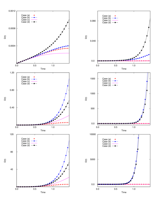
Figure 1: We show the comparison between diffusion coefficients for the different cases considered. Plots on the top refers to the case $\gamma_{0}=0$, in which the composite system is isolated from the external bath. Plots in the middle and at the bottom represent the coefficients for $\gamma_{0}k_{B}T=1$ and 100, respectively. On the left column: we use $\omega=\Omega=1$, $\sigma=0.01$. On the right column: $\omega=5\Omega$, $\sigma=0.01$. Cases (b) and (d) show a bigger growing rate at short times for both set of parameters.

In Fig. 1, we can appreciate the difference between the diffusion terms for composite systems when subsystem A is unstable and when it is not. In fact, the exponential behavior in the (b) and (d) cases is due to the fact that the final “decohered” subsystem A is unstable diana ; pau (the upside-down oscillator). On the contrary, cases (a) and (c) present an oscillatory behaviour since subsystem A is a harmonic oscillator (and the solution $x_{\rm cl}(s)$ for the classical equation of motion has oscillatory functions instead of hyperbolic function as in cases (b) and (d)). The difference between the exponential diffusion coefficients and the harmonic ones is particularly manifested for times $\omega t\geq 1$. For smaller times, all the coefficients are equivalent. But for longer times, cases (b) and (d) are easily dintinguishable from (a) and (c). The dynamics of the unstable upside-down oscillator is much in evidence after $\Omega t\geq 1$, where cases (b) and (d) start to differenciate each other.

The plots on top of Fig. 1, are a generalization of the results obtained by Blume-Kohout and Zurek robin in which they considered a harmonic oscillator coupled to an inverted oscillator as an unique environment (there was no coupling between subsystem B and the external reservoir, i.e. $\gamma_{0}=0$ in our model). Plots in the middle and at the bottom of the same figure are for small and high values of $\gamma_{0}k_{B}T$ since we have explicitly considered the presence of the external hot bath $\cal{E}$, and thus, this presence modifies the diffusion terms adding a new contribution with respect to the one obtained in Ref. robin .

In the case of $\gamma_{0}=0$, it is easy to note that ${\cal D}_{\rm d}$ (case (d)) grows faster (like an exponential function of time), while the other coefficients remain with a smaller amplitude. This is important in order to evaluate decoherence times, postponed till next Section. Instabilities inherent to the subsystem A exponentially enhance the diffusion originated due to the interaction with the environment. When the B-oscillator is also unstable, we have more exponential sensitivity to perturbations than in any other case. However, it is important to note that it is a very toy model, in the sense that both oscillators are unbounded from below and therefore will develop un-physical oscillatory divergences robin . Therefore, we conclude that in order to have a more precise idea of the physical consequences of having chaotic modes into the environment, we can not neglect the interaction of these chaotic degrees of freedom with the rest of the world, modelled here as an infinite set of harmonic oscillators.

The diffusion suffered by the subsystem A is the direct result of the interaction between A and B, and between the later and the external environment ${\cal E}$ when this last one is taken into account. The environment reacts to this interaction and the backreaction on the subsystem is by means of diffusion and dissipation. Let’s take for example cases (b) and (d): unstable subsystem A is coupled to a harmonic oscillator (case (b)) or to an upside-down oscillator (case (d)). Subsystem A handles information to B via their coupling. In case (b), as B-oscillator is harmonic, the diffusion process is more effective. The B-oscillator has an oscillatory behaviour in time and is able of providing subsystem A with diffusion periodically. On the contrary, in case (d), the B-oscillator is unstable and unbounded from below. The stretching of its states is boundless (see next Section). Thus, part of the information is transferred to the reservoir, but, at large times, the intrinsic dynamics of the upside-down oscillator makes the provision of subsystem A with diffusion scarce and, consequently, less effective. A more quantitative explanation will be given in the following Section, when we give an analytical estimation of the decoherence time for each case.

Cases (a) and (c) are slightly different. Subsystem A is harmonic and the environment can have an unstable degree of freedom (case (a)) or not (case (c)). It is easy to see in Figure 1 that the backreaction of the full environment (B + $\cal{E}$) on the subsystem A by means of the diffusion process is more effective for cases (b) and (d) (in this order) than for cases (c) and (a). This is due to the fact of having an inverted oscillator as the final subsystem A. In the middle of these figures, the “low temperature” limit is shown [we are still working in the high temperature limit, but we are considering the underdamped case ($\gamma_{0}$ is small with respect to any of the present frequencies), therefore the coefficient $\gamma_{0}k_{B}T$ could be a small number still preserving the hot bath assumption]. We can see that ${\cal D}_{\rm b}$ grows slightly faster than ${\cal D}_{\rm d}$, and both of them are bigger than ${\cal D}_{\rm a}$ and ${\cal D}_{\rm c}$. This can be understood by thinking in the dynamical properties of the composite system coupled to the external bath as we mentioned above. Oscillator B is not a good “diffusion handler” if it is unstable. At times longer than $\Omega t>1$, states in this oscillator are spread out too much. Diffusion must go from ${\cal E}$ to A through B (middle-environment subsystem). It is not an effective process at short times (all the cases have a similar behaviour at short times). The dynamical behaviour of case (a) should be similar to the one occurring in case (b). However, the difference of having an inverted oscillator as the subsystem A or as the intermediate subsystem B is crucial. That is reflected in the exponential grow (or not) of the diffusion coefficient and in the decoherence times that we will present in the following Section.

As we stated before, in the (b) and (d) cases, the spreading of the initial state of the subsystem A is exponentially sensitive to fluctuations coming from the full environment (B + $\cal{E}$), and it reacts quickly on the bath, losing information faster than in any other case. This is what happens in case (b), although the middle-environment is a harmonic oscillator. However, a question might arise: why ${\cal D}_{\rm b}$ grows faster than ${\cal D}_{\rm d}$, if the latter is “twice” unstable?. The key is: case (b) is the most decoherent because the unstable system losses its information in an uniform (non-ohmic) environment composed by a harmonic oscillator (B) plus an infinite set of harmonic oscillators in thermal equilibrium without internal unbounded regions (contrary to what happens in case (d)). In the low-T example, the major contribution to diffusion comes from the intrinsic dynamics of the composite system alone. At early times ($\omega t<1$), unstable dynamics of the subsystem A dominates the temporal behaviour and, as they both have an inverted A oscillator, both cases (b) and (d) are similar (in fact, all the cases are similar at short temporal scales because at very short times both potentials are similar). However, when $\omega t\geq 1$, and the presence of the external environment is still not so important, there is a noteworthy difference between ${\cal D}_{\rm b}$ and ${\cal D}_{\rm d}$ when the frequency of the subsystem A is similar to the one of B (see middle of Fig. 1 on the left). When A has a bigger frequency, the dynamics is dominated by subsystem A and both diffusion coefficients are extremely similar in a longer temporal scale (middle Fig. 1 right). ${\cal D}_{\rm b}$ and ${\cal D}_{\rm d}$ are indistinguishable for $\omega>\Omega$ even at $\gamma_{0}k_{B}T\sim 1$. However, as the temperature of the thermal bath increases, there is no distinction between cases (b) and (d) because the external environment dominates the diffusion coefficient. At high values of $\gamma_{0}k_{B}T$ we obtain a clear hierarchy between different composite systems (Fig. 1 at the bottom). Again, it is easy to observe that the diffusion coefficients of those cases in which subsystem A is an upside-down oscillator reach bigger values than the others that have a harmonic oscillator as subsystem A. Therefore, we are able to conclude that the presence of instabilities into the composite system enhance decoherence. This effect is yet more important if the unstable subsystem A is coupled either to a solely chaotic degree of freedom (in the absence of external bath like our case (d)) or to an external environment (formed by B + $\cal{E}$) at high $\gamma_{0}k_{B}T$, as in cases (b) and (d). In Fig. 2 we present the diffusion coefficient at a high value of $\gamma_{0}k_{B}T$ for both systems which have a harmonic oscillator as subsystem A: cases (a) and (c). This figure should come in handy so as to compare these oscillatory coefficients with the hyperbolic-like other two.

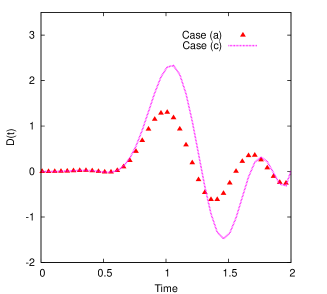
Figure 2: Diffusion coefficients for cases (a) and (c) with $\omega=5\Omega$, $\sigma=0.01$ and $\gamma_{0}k_{B}T=100$. We can see the evolution of these coefficients at larger times than in Fig. 1.

IV Decoherence in $A$ interacting with $B-{\cal E}$

After integrating out all the degrees of freedom corresponding to the external hot environment $Q_{n}$, and the coordinates $q$ belonging to the subsystem B, we obtained the diffusive terms that induce decoherence on subsystem A. Therefore, we numerically integrated the diffusive terms in time, in order to plot the decoherence factor (see Appendix)

$$\Gamma(t)=\exp\left\{-\int_{0}^{t}{\cal D}(s)~{}ds\right\}.$$ (36)

Thus, $\Gamma(t)$ is initially one (there is no interaction at $t=0$ between subsystems and environment), and it decays to zero with time (this is the case of total decoherence). From the master equation for A-subsystem, it is easy to see that factor $\Gamma(t)$ is at the root of the loss of quantum coherence. In order to illustrate the same cases, we present all four $\Gamma$ coefficients when both frequencies of the subsystems A and B are of the same order of magnitude ($\omega\approx\Omega$) and when $\omega>\Omega$, as shown in Fig. 3 on the left and right columns, respectively. Both cases are considered in the absence of external environment $\cal{E}$ (i.e. $\gamma_{0}=0$) and for low and high values of $\gamma_{0}k_{B}T$.

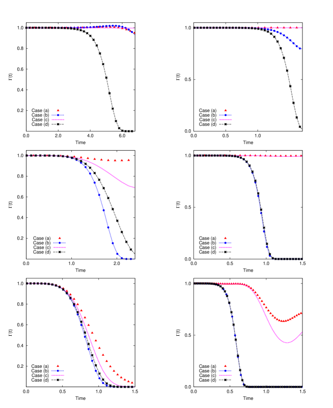
Figure 3: Decoherence factor for the same set than Fig. 1. Isolated composite system decoheres first for the (d) case. For $\gamma_{0}\not=0$, case (b) is more decoherent.

From the numerical results shown on top of Fig. 3, we can stress that in the absence of a hot bath, the decoherence time is smaller in case (d) than in (b), and both of them decohere long before cases (a) and (c). This is due to the fact that subsystem A, which is solely coupled to subsystem B, generates noise and dissipation at large scales. Thus, this noise and dissipation is bigger when the subsystem B is an upside-down oscillator (case (d)) than when it is a harmonic oscillator (case (b)). In this situation ($\gamma_{0}=0$), case (d) is twofold exponential in time. In these figures, we can also observe what is going on for cases (a) and (c). In the former, the oscillatory dynamics of the A-oscillator and the hyperbolic stretching of the B-environment, proceed largely independently of one another. The B-environment induces only minor perturbations in the subsystem A and this subsystem does not disturb the environment. The stretching of the environment (due to being an inverted oscillator) along its unstable manifold is reflected in the system as diffusion. The same physical process occurs in case (b), with the sole and essential difference that the one stretching along an unstable direction is the subsystem A, while the environment is oscillating. As this stretching results in diffusion, the more stretching the system has, the more diffusion it feels. Case (d) is the best example in this “isolated” model, because both, A and B, stretch along a direction in the phase space, producing double exponential diffusion. This is the reason why it is the most decoherent case. Case (c) is shown for completeness, but it is easily seen that decoherence occurs in a longer time scale (there is no stretching here).

As soon as the interaction between B and the thermal environment is switched on, oscillator B dissipates not only on the bath but also on A. This is shown in the middle and at the bottom of Fig. 3. At very high environmental temperatures, there is no difference between cases (b) and (d); both of them decohere in the same temporal scale. The huge reservoir dominates the diffusion terms. But they still differ from the cases where there are harmonic oscillators as subsystems A (cases (a) and (c)). In Figure 4 we present the behaviour of the $\Gamma(t)$ coefficients for these cases for a longer time scale. We can observe that we need to wait longer times for decoherence to be effective in cases (a) or (c) with respect to (b) and (d) even in the highest temperature case.

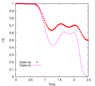
Figure 4: Cases (a) and (c) for $\gamma_{0}k_{B}T=100$, $\omega=5\Omega=5$. Here we can see that, even the behaviour of $\Gamma(t)$ is similar, case (c) decoheres first than case (a), in which B-system is an inverted oscillator.

IV.1 Decoherence time predictions

In this Section we will present an analytical estimation of the decoherence times based on the inverted oscillators’ unstable dynamics of the phase space.

When the final system A is an upside-down oscillator ZP , an unstable point forms in the center of the phase space with associated stable and unstable directions. These are characterized by Lyapunov coefficients $\Lambda$ with negative and positive real parts respectively. In order to have a quantitative expression for decoherence times we have to take into account that the dynamics now gives raise to the possibility of squeezing along the stable direction. The exponential stretching of the Gaussian packets in one of the directions due to the hyperbolic point is compensated by an exponential squeezing. The time dependence of the package width in the direction of the momenta is given by $\sigma_{p}(t)=\sigma_{p}(t_{0})\exp{[\Lambda t]}$, where $\sigma_{p}(t_{0})$ is the corresponding width at the initial time. Lyapunov coefficient is given by the value corresponding to a linear potential $\Lambda=2\omega^{2}$.

Diffusion effects limit the squeezing of the Wigner function. The bound on the width of the packets is given by $\sigma_{\rm c}=\sqrt{2{\cal D}_{\rm i}/\Lambda}$ JPP-LH ; habib (where ${\rm i}$ is b or d). There is another scale, $t_{\rm max}$ corresponding to the time in which decoherence starts to be effective, and after which squeezing becomes of the order of the limiting value. We use this to estimate the decoherence time scale.

Evolution of the Gaussian packet will typically proceed in two different stages. During the first stage, evolution is dominated by the unitary part of the master equation and will be within an approximately preserved area. This lasts the time needed for the spreading of the initial state over a regular patch to be larger than the critical width. During this stage diffusion does not alter much the Wigner function, which is stretched or contracted. When the dimension of the patch becomes comparable with $\sigma_{\rm c}$, diffusion begins to dominate and the second stage of evolution begins. Further contraction will be halted at $\sigma_{\rm c}$ but the stretching will proceed at the rate set by the positive Lyapunov exponent. As a result, the area (or the volume) in phase space increases. One can estimate the time corresponding to the transition from reversible to irreversible evolution as

$$t_{\rm c}=\frac{1}{\Lambda}\ln{\frac{\sigma_{p}(0)}{\sigma_{\rm c}}}.$$ (37)

In our toy model, we can use this scale as the typical scale for decoherence, setting $t_{D}\approx\frac{1}{\Lambda}\ln{\frac{\sigma_{p}(t_{\rm max})}{\sigma_{\rm c}}}$, therefore we obtain

$$t_{D}=t_{\rm max}+\frac{1}{\Lambda}\ln{\frac{\sigma_{p}(0)}{\sigma_{\rm c}}}.$$ (38)

For the same parameters used in Fig. 3, we are able to numerically estimate decoherence times as: $t_{D_{\rm b}}\sim 7.7$ and $t_{D_{\rm d}}\sim 6.4$, for the first set of parameters on the left of Fig. 3 ($\omega=\Omega=1$) where $\gamma_{0}=0$; $t_{D_{\rm b}}\sim 2.4$ and $t_{D_{\rm d}}\sim 2.7$; for $\gamma_{0}k_{B}T=1$, and $t_{D_{\rm b}}\sim 1.6$ and $t_{D_{\rm d}}\sim 1.7$, in the hight T case $\gamma_{0}k_{B}T=100$. For the set on the right Fig. 3 ($\omega=5\Omega=5$), we estimated: for $\gamma_{0}=0$; $t_{D_{\rm b}}\sim 3.0$ and $t_{D_{\rm d}}\sim 2.7$. We also got $t_{D_{\rm b,d}}\sim 0.1$, for $\gamma_{0}k_{B}T=1$, and $t_{D_{\rm b,d}}\sim 0.6$ in the case $\gamma_{0}k_{B}T=100$. All these results agree with the decoherence times, defined by the times the decoherence factor $\Gamma(t)$ goes to zero, that can be seen in the figures above.

Using Eq.(37), we can check that decoherence proceeds slower in case (d) than in case (b) for $\gamma_{0}\not=0$,

$$t_{D_{\rm b}}-t_{D_{\rm d}}=\frac{1}{\Lambda}\ln{\frac{\sigma_{\rm c}^{\rm d}}{\sigma_{\rm c}^{\rm b}}}=\frac{1}{2\Lambda}\ln{\frac{{\cal D}_{\rm d}}{{\cal D}_{\rm b}}}.$$ (39)

By simple inspection of diffusion coefficients in the figures, we can see that ${\cal D}_{\rm d}<{\cal D}_{\rm b}$ implying $t_{D_{\rm b}}<t_{D_{\rm d}}$.

In the isolated from external environment case ($\gamma_{0}=0$), we have ${\cal D}_{\rm d}>{\cal D}_{\rm b}$ resulting in $t_{D_{\rm b}}>t_{D_{\rm d}}$, which agrees with our qualitative arguments and with what is shown in the plots on top of Fig. 3.

Decoherence times for cases (a) and (c) occur as for the usual harmonic systems. We can estimate them by using the result of the high temperature limit of the quantum Brownian motion paradigm, i.e. $t_{D}$ is the solution of: $1\approx L^{2}\int_{0}^{t_{D}}{\cal D}(s)ds$ (we have to take the typical distance $L$ as $2\sigma$, proportional to the dispersion in position of our initial Gaussian packet). We present, in Fig. 4, $\Gamma(t)$ for a longer time scale in order to establish the corresponding hierarchy in the environmental decoherent effectiveness.

V Final remarks

In this article we analyzed the decoherence induced by an effective environment. The effective environment was considered to be formed by part of a composite system and an infinite set of harmonic oscillators. The composite system was considered to be any of the four possible combinations made up with a harmonic and an inverted oscillator.

Since a set of harmonic oscillators is a stable system, small perturbations due to the state of the coupled system do not induce exploration of a large volume of the phase space for any oscillator. When one considers an inverted oscillator, it can explore its volume more efficiently when it is perturbed.

When one works with a composite quantum open system in interaction with an stable environment, it is almost probed that the composite system (or part of it, for example its unstable degrees of freedom) will decohere before those systems where there are not inverted potentials (like our case (c)). Therefore, one could have a mixture of quantum-classical dynamics for the open composite system due to the fact that the different parts of the global system loss coherence at different rates.

In our article we integrated out subsystem B, in order to study the effect of having (or not) unstable degrees of freedom into the full environment. Then we analyzed different situations and concluded that cases (b) and (d) are the most efficient (smaller decoherence times) at high temperatures, and (d) is the most diffusive case, when one turns off the thermal bath. There is a clear hierarchy between the different compositions of the composite systems. Those in which oscillator A is unstable (cases (b) and (d)) decohere before than those with a harmonic oscillator as the A-subsystem (cases (a) and (c)). At high temperatures of the external environment, it has been shown that cases (b) and (d) have the same decoherence time scale, while composite system (c) losses quantum coherence before case (a).

As the system and environment interact, information about the initial state of the subsystem A is transferred to the environment (and vice-verse). Case (b) is the most decoherent because the unstable system losses its information in an uniform (non-ohmic) environment composed by an harmonic oscillator (B) plus an infinite set of harmonic oscillators in thermal equilibrium without internal unstable (and unbounded) regions (contrary to what happens in case (d)). At intermediate temperatures, unstable A-subsystems decohere before stable A-subsystems because the intrinsic dynamics of those subsystems produce exponentially driven diffusive terms. However, at high temperatures the environment does not distinguish between subsystems and decoherence proceeds equally in every case. The effectiveness of diffusion depends on the intermediate-environment subsystem B. We have shown that harmonic oscillators keep information during a major period of time and therefore are able to react on the A-system more efficiently, than the case in which one has an inverted oscillator as “information delivery subsystem”. This is the main reason why case (b) is more decoherent (in general) than case (d), and why case (c) is more effective losing quantum coherence than case (a). It is important to stress that in order to have a more physical model for the effective environment which would contain an unstable degree of freedom one should consider a double well potential as B-oscillator. For example, for cases (a) or (d). This non-linear potential has all the unstable properties of the upside-down oscillator at early times (giving a contribution to the diffusion terms which is exponential with time). Furthermore, this potential is bounded, which would be of much relevance in order to evaluate its global effect on subsystem A. In this situation, case (d) would be the most decoherent case at any value of $\gamma_{0}k_{B}T$ fut .

As was emphasized by authors of Ref. robin , the scale associated with the decoherence process when upside-down oscillators are taken into account as part of the coupled system, is logarithmically dependent on the coupling constant. This is easy to see from our analytical results, using the expression of the diffusion coefficient ${\cal D}$, given in the Appendix (Eq.(53)), into Eq.(38). This implies that isolation from chaotic environments is “exponentially” difficult. It is even harder to isolate a system (or subsystem) from a chaotic environment than from the many harmonic oscillators of the quantum Brownian motion environment, where decoherence time is quadratic in the coupling constant.

VI Acknowledgments

We thank Juan Pablo Paz for useful discussions. We also thank F.D. Mazzitelli and W.H. Zurek for comments during the early stage of this work. This work was supported by UBA, CONICET, Fundación Antorchas, and ANPCyT, Argentina.

Appendix A Derivation of the diffusion coefficient

In this Section, we show the calculation of diffusion coefficient corresponding to case (a), in which we have a harmonic oscillator coupled to an upside-down oscillator, and it is in interaction with a set of infinite harmonic oscillators at temperature T.

In order to perform the functional integrations of Eq.(24), we must solve the classical equation of motion for the subsystem B. If this system satisfies, $\ddot{q}(s)-\Omega^{2}q(s)=\frac{\lambda}{M_{\rm B}}x(s)$. The complete solution to this equation, after imposing initial and final conditions $q(s=0)=q_{0}$ and $q(s=t)=q_{\rm f}$, is given in Eq.(26).

Once we have the classical solution for the upside-down oscillator coupled to a subsystem of coordinate $x(s)$, we can write explicitly the influence action obtained after integrating out all the degrees of freedom of the environment $\cal E$ (Eq.(18)). Neglecting the action of dissipation into the influence action (the dissipation coefficient $\gamma_{0}$ is basically the square of the coupling constant between subsystem $B$ and the environment ${\cal E}$, [$\gamma_{0}\approx c_{n}^{2}$] and we are working in the underdamped and high temperature limit ($\gamma_{0}<\omega,\Omega<k_{B}T$)), we can write it as

$$\delta A(q,q\prime)=i2M_{\rm B}\gamma_{0}KT\int_{0}^{t}ds(\Delta q(s))^{2}.$$ (40)

In last equation, $\Delta q(s)$ is given by

$$\Delta q_{\rm cl}(s)=(q_{0}-q_{0}\prime)^{2}\bigg{(}\frac{\sinh(\Omega(t-s))}{\sinh(\Omega t)}\bigg{)}^{2}+2(q_{0}-q_{0}\prime)\frac{\sinh(\Omega(t-s))}{\sinh(\Omega t)}g(s,t)+g(s,t)^{2},$$ (41)

with

$$g(s,t)=\frac{\lambda}{M_{\rm B}\Omega}\bigg{(}-\int_{0}^{s}du\Delta x(u)\sinh(\Omega(s-u))+\frac{\sinh(\Omega s)}{\sinh(\Omega t)}\int_{0}^{t}du\Delta x(u)\sinh(\Omega(t-u))\bigg{)}$$ (42)

and $\Delta x(u)=x(u)-x\prime(u)$. As the last term in expression (42) does not depend on the initial conditions, it will be transparent to integrals in Eq. (24). It is important to note that as subsystem $B$ is an upside-down oscillator with frequency $\Omega$, all the time-dependent functions in Eq. (42) are hyperbolic trigonometric functions.

After imposing $\rho_{\rm B}(q_{0},q_{0}\prime;0)=Ne^{-((q_{0}-q_{0}\prime)^{2})/2\sigma}$ as the initial wave packet for subsystem $B$, the expression for the influence functional is

$${\cal F}(x,x^{\prime}) = \exp\left\{{{i\over{\hbar}}\delta A(q,q^{\prime})}\right\}=\int_{-\infty}^{+\infty}dq_{\rm f}\int_{-\infty}^{+\infty}dq_{0}\int_{-\infty}^{+\infty}dq_{\rm f}^{\prime}\int_{q_{0}}^{q_{\rm f}}{\cal D}q\int_{q_{0}^{\prime}}^{q_{\rm f}^{\prime}}{\cal D}q^{\prime}e^{\frac{i}{\hbar}\delta A(q_{\rm cl},q_{\rm cl}\prime)}\ \rho_{\rm r}^{\rm B}(q_{0},q_{0}^{\prime})$$ (43)

$$\times e^{{i\over{\hbar}}(S_{\rm B}(q_{\rm cl})+S_{\rm AB}(x,q_{\rm cl})-S_{\rm B}(q^{\prime}_{\rm cl})-S_{\rm AB}(x^{\prime},q^{\prime}_{\rm cl}))},$$

where $q_{\rm cl}(s)$ is given in Eq.(26) and $\delta A(q,q\prime)$ in Eq. (40). Therefore, this integration can be done and yields (for a weakly coupled composite AB system) the result shown in Eqs.(27) and (28).

Once the influence functional is known, it is straightforward to write down the reduced density matrix for subsystem $A$ only

$$\rho_{\rm r}(x_{\rm f},x_{\rm f}\prime;t)=\int_{-\infty}^{\infty}dx_{0}\int_{-\infty}^{\infty}dx_{0}\prime\int_{x_{0}}^{x_{\rm f}}{\cal D}x\int_{x_{0}^{\prime}}^{x_{\rm f}^{\prime}}{\cal D}x^{\prime}e^{\frac{i}{\hbar}(S_{\rm A}(x)-S_{\rm A}(x\prime))}e^{-g^{2}(s,t)}e^{\frac{i}{\hbar}\delta{\cal A}(x,x\prime)}\rho_{\rm A}(x_{0},x_{0}\prime,0),$$ (44)

and the reduced evolution operator

$${\cal J}_{\rm r}(x_{\rm f},x_{\rm f}\prime;t|x_{0},x_{0}\prime;0)=\int_{x_{0}}^{x_{\rm f}}{\cal D}x\int_{x_{0}\prime}^{x_{\rm f}\prime}{\cal D}x\prime e^{\frac{i}{\hbar}(S_{\rm A}(x)-S_{\rm A}(x\prime))}e^{-g^{2}(s,t)}e^{\frac{i}{\hbar}\delta{\cal A}(x,x\prime)}.$$ (45)

In order to evaluate Eq.(45), we need the solution to the free equation of motion for subsystem A $\ddot{x}(s)+\omega^{2}x(s)=0$. If we ask for initial and final conditions of the form $x(s=0)=x_{0}$ and $x(s=t)=x_{\rm f}$, the classical solution is, $x_{\rm cl}(s)=x_{0}\frac{\rm{\sin}(\omega(t-s))}{\rm{\sin}(\omega t)}+x_{\rm f}\frac{\rm{\sin}(\omega s)}{\rm{\sin}(\omega t)}$, and the reduced evolution operator becomes

$${\cal J}_{\rm r}(x_{\rm f},x_{\rm f}\prime;t|x_{0},x_{0}\prime;0)=e^{\frac{i}{\hbar}(S_{\rm A}(x_{\rm cl})-S_{\rm A}(x\prime_{\rm cl}))}e^{-g^{2}(s,t)}e^{\frac{i}{\hbar}\delta{\cal A}(x,x\prime)}\equiv~{}e^{\frac{i}{\hbar}U(t)}e^{-D(t)}.$$ (46)

with U and D, related to the unitary evolution and decoherence process respectively, given by,

$$U=(x_{0}-x_{0}\prime)\frac{\rm{\sin}(\omega(t-s))}{\rm{\sin}(\omega t)}+(x_{\rm f}-x_{\rm f}\prime)\frac{\rm{\sin}(\omega s)}{\rm{\sin}(\omega t)}-2\gamma_{0}\int_{0}^{t}ds_{1}\int_{0}^{s_{1}}ds_{2}y(s_{1})\tilde{\eta}(s_{1}-s_{2})r(s_{2}),$$

and

$$D=\frac{2\gamma_{0}k_{B}T}{\hbar\Omega^{2}}\lambda^{2}\int_{0}^{t}ds(\Delta q(s))^{2}+\frac{\lambda^{2}}{32\hbar\sigma}\int_{0}^{t}ds_{1}\int_{0}^{s_{1}}ds_{2}y(s_{1})\tilde{\nu}(s_{1}-s_{2})y(s_{2}).$$

Following the same techniques used for the quantum Brownian motion Hu to obtain the master equation, we must compute the time derivative of the propagator ${\cal J}_{\rm r}$ Eq.(46), and eliminate the dependence on the initial conditions $x_{0}$, $x_{0}\prime$ that enters through the classical solution $x_{\rm cl}(s)$. This can be easily done using the properties of the solution

$$\Delta_{0}J_{\rm r}(t,0)=\left[\cos(\omega(t-s))\Delta_{\rm f}+\frac{\sin(\omega(t-s))}{\omega}i\hbar\frac{\partial}{\partial\Sigma_{\rm f}}\right]J_{\rm r}(t,0)$$ (47)

where $\Delta_{0}=(x_{0}-x_{0}\prime)$, $\Delta_{f}=(x_{f}-x_{f}\prime)$ and $\Sigma_{f}=(x_{\rm f}+x_{\rm f}\prime)$. This identity allows us to remove the initial coordinates $x_{0}$, $x_{0}^{\prime}$ by expressing them in terms of the final coordinates $x_{\rm f}$, $x_{\rm f}^{\prime}$ and the derivatives $\partial_{x_{\rm f}},\partial_{x_{\rm f}^{\prime}}$, and obtain the master equation.

The full equation is very complicated and, like in the case of the quantum Brownian motion, it depends on the system-environment coupling. In the present case, it also depends on the subsystems coupling constant $\lambda$. As we are solely interested in decoherence, it is sufficient to calculate the correction to the usual unitary evolution coming from the noise kernel (imaginary part of the influence action). The result reads

$$\dot{\rho}_{\rm r}(x_{\rm f},x_{\rm f}^{\prime};t) \sim -i[H_{\rm ren},\rho_{\rm r}]-\frac{\partial}{\partial t}\bigg{(}\frac{2\gamma_{0}k_{B}T}{\hbar}\frac{\lambda^{2}}{\Omega^{2}}\int_{0}^{t}ds~{}g(s)^{2}-\int_{0}^{t}\int_{0}^{s}dsds^{\prime}\Delta x_{\rm cl}(s)\tilde{\nu}(s,s^{\prime})\Delta x_{\rm cl}(s^{\prime})\bigg{)}\rho_{\rm r}+...$$

$$= -i[H_{\rm ren},\rho_{\rm r}]-\bigg{(}\frac{2\gamma_{0}KT}{\hbar}\frac{\lambda^{2}}{\Omega^{2}}\int_{0}^{t}2\dot{g}(s)g(s)ds+\frac{\lambda^{2}\sigma}{32\hbar}(x_{\rm f}-x_{\rm f}^{\prime})\int_{0}^{t}ds\cosh(\Omega(t-s))\Delta x_{\rm cl}(s)\bigg{)}\rho_{\rm r}$$

$$+ ...,$$

where ellipsis denote other terms that do not contribute to decoherence.

This is equivalent to write

$$\dot{\rho_{\rm r}}\approx-i[H_{\rm ren},\rho_{\rm r}]-(x_{\rm f}-x_{\rm f}^{\prime})^{2}{\cal D}(t)\rho_{\rm r},$$ (48)

with $\cal{D}$ the diffusion coefficient (Eq.(53)). Then, the effect of the diffusion coefficient on the decoherence process can be seen considering the following approximate solution to the master equation

$$\rho_{\rm r}(x_{\rm f},x_{\rm f}^{\prime};t)\approx\rho_{\rm r}^{\rm u}(x_{\rm f},x_{\rm f}^{\prime};t)~{}e^{-(x_{\rm f}-x_{\rm f}^{\prime})^{2}\int_{0}^{t}{\cal D}(s)ds},$$ (49)

where $\rho_{\rm r}^{\rm u}$ is the solution to the unitary part of the master equation ( i.e., without environment). The system will decohere when the non-diagonal elements of the reduced density matrix are much smaller than the diagonal ones.

For the case of a harmonic oscillator coupled to an upside-down oscillator, which is coupled to an external environment, the diffusion coefficient (Eq.(53)) for total the reduced density matrix $\rho_{\rm r}(x_{\rm f},x_{\rm f}^{\prime};t)$ is

$${\cal D}_{\rm a} = \frac{\Omega^{2}}{(\omega^{2}+\Omega^{2})^{2}}\Big{\{}\frac{2\gamma_{0}k_{B}T}{\hbar\Omega^{2}}\lambda^{2}\int_{0}^{t}ds\Big{[}\frac{\sinh(\Omega s)}{\sinh(\Omega t)}(\cosh(\Omega t)\cos(\omega t)-1)-\cosh(\Omega s)\cos(\omega t)+\cos(\omega(t-s))\Big{]}$$ (50)

$$\times \Big{[}\Omega\Big{(}\frac{\sinh(\Omega s)}{\sinh(\Omega t)^{2}}\cosh(\Omega t)(1-\cosh(\Omega t)\cos(\omega t))+\sinh(\Omega s)\cosh(\omega t)\Big{)}+\omega\Big{(}-\frac{\sinh(\Omega s)}{\sinh(\Omega t)}\sin(\omega t)\cosh(\Omega t)$$

$$- \sin(\omega(t-s))+\sin(\omega t)\cosh(\Omega s)\Big{)}\Big{]}+\frac{\lambda^{2}\sigma}{32\hbar}\int_{0}^{t}ds\cosh(\Omega(t-s))\cos(\omega(t-s))\Big{\}}.$$

The procedure to evaluate the diffusion term for case (b), when one has an upside-down oscillator coupled to a harmonic one, and the last to the environment, is equivalent to what was done in the Subsection above but replacing $\Omega\rightarrow i\Omega$ and $\omega\rightarrow i\omega$. This is because subsystem $B$ satisfies ${\ddot{q}}(s)+\Omega^{2}q(s)=\frac{\lambda}{M_{\rm B}}x(s)$ and subsystem $A$ satisfies ${\ddot{x}}(s)-\omega^{2}x(s)=0$.

Therefore, in this case, $q_{\rm cl}(s)$ is,

$$q_{\rm cl}(s) = q_{0}\frac{\rm{\sin}(\Omega(t-s))}{\rm{\sin}(\Omega t)}+q_{\rm f}\frac{\rm{\sin}(\Omega s)}{\rm{\sin}(\Omega t)}-\frac{\lambda}{M_{\rm B}\Omega}\frac{\rm{\sin}(\Omega s)}{\rm{\sin}(\Omega t)}\int_{0}^{t}x(u)\rm{\sin}(\Omega(s-u))du$$ (51)

$$+ \frac{\lambda}{M_{B}\Omega}\int_{0}^{s}x(u)\rm{\sin}(\Omega(s-u))du,$$

and $x_{\rm cl}(s)$,

$$x_{\rm cl}(s)=x_{0}\frac{{\sinh}(\omega(t-s))}{{\sinh}(\omega t)}+x_{\rm f}\frac{{\sinh}(\omega s)}{{\sinh}(\omega t)}.$$ (52)

If one follows all the procedure detailed above one obtains as the diffusion coefficient,

$${\cal D}_{\rm b} = \frac{\Omega^{2}}{(\omega^{2}+\Omega^{2})^{2}}\Big{\{}\frac{2\gamma_{0}k_{B}T}{\hbar\Omega^{2}}\lambda^{2}\int_{0}^{t}ds\Big{[}\frac{\sin(\Omega s)}{\sin(\Omega t)}(\cos(\Omega t)\cosh(\omega t)-1)-\cos(\Omega s)\cosh(\omega t)+\cosh(\omega(t-s))\Big{]}$$ (53)

$$\times \Big{[}\Omega\Big{(}\frac{\sin(\Omega s)}{\sin(\Omega t)^{2}}\cos(\Omega t)(1-\cos(\Omega t)\cosh(\omega t))+\sin(\Omega s)\cos(\omega t)\Big{)}+\omega\Big{(}-\frac{\sin(\Omega s)}{\sin(\Omega t)}\sinh(\omega t)\cos(\Omega t)$$

$$- \sinh(\omega(t-s))+\sinh(\omega t)\cos(\Omega s)\Big{)}\Big{]}+\frac{\lambda^{2}\sigma}{32\hbar}\int_{0}^{t}ds\cos(\Omega(t-s))\cosh(\omega(t-s))\Big{\}}.$$

Diffusion terms ${\cal D}_{\rm c}$ and ${\cal D}_{\rm d}$ can be obtained in a similar way, by replacing $\Omega\rightarrow i\Omega$ in ${\cal D}_{\rm a}$ and ${\cal D}_{\rm b}$, respectively.

References

- (1) W.H. Zurek, Rev. Mod. Phys. 75, 715 (2003)
- (2) E.B. Davies, Quantum Theory of Open Systems (Academic, London, 1976); B.J. Lindenberg and B.J. West, The Nonequilibrium Statistical Mechanics of Open System (VCH, New York, 1990); U. Weiss, Quantum Dissipative Systems (World Scientific, Singapore, 1999)
- (3) F.C. Lombardo and F.D. Mazzitelli, Phys. Rev. D53, 2001 (1996); F.C. Lombardo, F.D. Mazzitelli, and R.J. Rivers, Phys. Lett. B523, 317 (2001); F.C. Lombardo, F.D. Mazzitelli, and R.J. Rivers, Nucl. Phys. B672, 462 (2003)
- (4) O.V. Prezhdo and P. Rossky, Phys. Rev. Lett. 81, 5294 (1998)
- (5) J.P. Paz and W.H. Zurek, Environmet-induced decoherence and the transition from quantum to classical, lectures at the 72nd Les Houches Summer School on ”Coherent Matter Waves”; (1999). arXiv: quant-ph/0010011
- (6) M. Toutounji and R. Kapral, Chem. Phys, 268, 79 (2001); O.V. Prezhdo, Phys. Rev. A56, 162 (1997)
- (7) R. Blume-Kohout and W.H. Zurek, Phys. Rev. A68, 032104 (2003)
- (8) Hans-Thomas Elze, Vacuum-Induced Quantum Decoherence and the Entropy Puzzle; hep-ph/9407377
- (9) F.C. Lombardo, F.D. Mazzitelli, and D. Monteoliva, Phys. Rev. D62, 045016 (2000); N.D. Antunes, F.C. Lombardo, and D. Monteoliva, Phys. Rev. E64, 066118 (2001)
- (10) K. Shiokawa and R. Kapral, J. Chem. Phys. 117, 7852 (2002)
- (11) A. Venugopalan, Phys. Rev. A61, 012102 (1999)
- (12) F.C. Lombardo and P.I. Villar, Phys. Rev. A72, 034103 (2005)
- (13) R.P. Feynman and F.L. Vernon, Ann. Phys. (N:Y:) 24, 118 (1963)
- (14) B.L. Hu, J.P. Paz, and Y.Zhang, Phys. Rev. D45, 2843 (1992)
- (15) H. Grabert, P.Schramm, G.L.Ingold: Phys. Rep. 168,115 (1988)
- (16) J.P. Paz, S. Habib, and W.H. Zurek, Phys. Rev. D47, 488 (1993)
- (17) B.L. Hu, J.P. Paz, and Y.Zhang, Phys. Rev. D47, 1576 (1993)
- (18) F.C. Lombardo and P.I. Villar, Phys. Lett. A336, 16 (2005)
- (19) W.H. Zurek and J.P. Paz, Phys. Rev. Lett. 72, 2508 (1994)
- (20) F.C. Lombardo and P.I. Villar, in preparation