Matrix Element Distributions as a Signature of Entanglement Generation

Abstract

We explore connections between an operator’s matrix element distribution and its entanglement generation. Operators with matrix element distributions similar to those of random matrices generate states of high multi-partite entanglement. This occurs even when other statistical properties of the operators do not conincide with random matrices. Similarly, operators with some statistical properties of random matrices may not exhibit random matrix element distributions and will not produce states with high levels of multi-partite entanglement. Finally, we show that operators with similar matrix element distributions generate similar amounts of entanglement.

Entanglement, correlations between quantum systems beyond what is classically possible, is an essential phenomenon in quantum information processing and a necessary resource for quantum communication. In the space of pure states, the overwhelming majority are of high multi-partite entanglement with respect to a qubit architecture Scott . Such states are necessary for quantum protocols calling for random, highly entangled states including superdense coding Aram , remote state preparation Bennet , and data hiding schemes Hayden .

Random states can be produced on a quantum computer by applying random unitary operators to computational basis states. However, the implementation of operators drawn randomly from the space of all unitary operators, the circular unitary ensemble (CUE), is very inefficient. Instead, other operators have been suggested as possibly efficient substitutes for the production of random, highly entangled states. These include quantum chaotic operators WGSH and pseudo-random operators RM ; QCARM ; CRM . However, these operators are not truly random and thus do not uniformly cover the space of pure states. Here we attempt to identify what statistical properties of random matrices lead to the production of highly entangled, random states. Identification of such a link between entanglement and randomness provides a deeper understanding of entanglement. In addition, isolating these properties may focus the search for operators with the ability to efficiently produce random states. Such operators need only fulfill the identified statistical properties and can fall short of CUE in regards to other statistical distributions.

In this paper we suggest that the element distribution of a given operator is a vital statistical property when attempting to create highly entangled states. To demonstrate this we first show that the larger percentage of CUE covered by a given ensemble, the more the matrix element distribution converges to CUE and so does the entanglement generation. Of course, this will generally cause other properties to also approach CUE. We then isolate various statistical properties through the use of operators which have certain statistical properties similar to CUE but not others. This disconnects the matrix elements from other statistical properties and shows their primacy in entanglement production. Specifically, an operator may not produce CUE-levels of entanglement if the matrix element distribution does not follow CUE, despite having other statistical similarities to CUE. Also, CUE-like entanglement production can be achieved with operators that have CUE-like matrix element distributions even if other statistical properties do not follow CUE. We note that not all of the operators we explore can be efficiently implemented on a quantum computer. Rather, the goal is to understand how certain operators can produce states with high levels of entanglement. This work concentrates on the matrix element distribution without exploring higher order correlations between the elements. These correlation may also play an important role in entanglement generation and will be the subject of further study. We have briefly mentioned the importance of the matrix elements to entanglement generation in Ref. YSW .

The operator classes used in this work to demonstrate all of the above, are (1) the interpolating ensembles Zyc3 , a one-parameter family of ensembles which interpolate between diagonal matrices with uniform, independently distributed elements, and CUE, (2) pseudo-random operators RM proposed as possibly efficient substitutes for random matrices, and (3) quantum chaotic operators which are generally known to have many statistical properties similar to random matrices BGS .

CUE matrices can be generated by multiplying eigenvectors of a Hermitian matrix belonging to the Gaussian unitary ensemble (GUE) by a random phase and using the resulting vectors as the CUE matrix columns Zyc2 . Thus, the squared modulus, or amplitude, of CUE matrix elements follows a distribution equal to that of GUE eigenvector element amplitudes. Let $c^{l}_{k}$ denote the $k$th component of the $l$th GUE eigenvector. The distribution of amplitudes, $\eta=|c^{l}_{k}|^{2}$, is

$$\tilde{P}_{GUE}(\eta)=(N-1)(1-\eta)^{N-2},$$ (1)

where $N$ is the Hilbert space dimension. In the limit $N\rightarrow\infty$, after rescaling to unit mean, the distribution is given by

$$P_{GUE}(y)=e^{-y},$$ (2)

where $y=N\eta$ Zyc . Since $\eta$ is unchanged when multiplied by a phase, the distribution, $P_{CUE}(x)$, of the rescaled amplitude of CUE matrix elements $x$, is equal to $P_{GUE}(y)$.

As a practical measure of multi-partite entanglement for an $n$-qubit system, we explore the average bipartite entanglement between each qubit and the rest of the system Meyer ; Bren2 ,

$$Q=2-\frac{2}{n}\sum^{n}_{j=1}Tr[\rho_{j}^{2}],$$ (3)

where $\rho_{j}$ is the reduced density matrix of qubit $j$. In this work, we study the distribution of $Q$ after one iteration of an operator as compared to the distribution of $Q$ for CUE matrices, $P_{CUE}(Q)$, and the average entanglement as a function of time, $\langle Q(t)\rangle$, compared to the CUE average entanglement Scott

$$\langle Q\rangle_{CUE}=(N-2)/(N+1).$$ (4)

CUE matrices can also be generated based on the Hurwitz parameterization Zyc2 and a modification of this construction is used to generate the interpolating ensembles. The interpolating ensembles are a one-parameter, family of ensembles which interpolate between diagonal matrices with uniform, independently distributed elements, and CUE. The parameter, $\delta$, can take on any value between 0, representing diagonal matrices, and 1, for CUE matrices. The exact method for the construction of CUE matrices via the Hurwitz parameterization and the modifications needed for the interpolating ensembles is reviewed in Appendix A. Interpolating ensembles have proved useful in analyzing certain scattering matrices Zyc4 ; SB and a quantum electron pump CB . One of the attractive features of these ensembles is that their eigenvalue and eigenvector properties have only a weak dependence on $N$. The matrix elements for these operators, however, show a strong dependence on $N$ and this, in turn, effects their entangling power.

Pseudo-random matrices RM ; CRM ; QCARM are operators that were proposed as possible efficient replacements of inefficient random operators in quantum information protocols. To implement a pseudo-random operator apply $m$ iterations of the $n$ qubit gate: random $SU(2)$ rotation to each qubit, then evolve the system via all nearest neighbor couplings RM . A random $SU(2)$ rotation is described by Eqs. (A) and (11). The nearest neighbor coupling operator used is:

$$U_{nnc}=\exp(i\frac{\pi}{4}\sum^{n-1}_{j=1}\sigma_{z}^{j}\otimes\sigma_{z}^{j+1}),$$ (5)

where $\sigma_{z}^{j}$ is the $j$th qubit $z$-direction Pauli spin operator. The random rotations are different for each qubit and each iteration, but the coupling constant is always $\pi/4$ to maximize entanglement generation. After the $m$ iterations, a final set of random rotations is applied.

Reference YSW discusses various statistical properties of both these operator classes in connection with entanglement production. Some of these properties are displayed here for completion. Figs. 1 and 2 show nearest neighbor eigenangle spacings (the more intricate number variance is provided in Ref. YSW ), eigenvalue element distribution, matrix element distribution and one-iteration entanglement distribution for the interpolating ensemble matrices and pseudo-random operators for constant $N$. As the operators cover more of CUE, $\delta\rightarrow 1$ and $m\rightarrow\infty$, the various properties including the matrix element distribution and the entanglement generation approach CUE distributions, as expected. We note however, that the matrix elements and entanglement generation appear to approach CUE more slowly than the other properties leading us to suspect that there may be a connection. This is born out by rewriting the average of $Q$ in terms of the elements of the wavefunction

$$\langle Q\rangle=4\big{(}\sum^{N/2}_{m=1}\sum^{N}_{n=\frac{N}{2}+1}\langle|c_{m}|^{2}|c_{n}|^{2}\rangle-\sum^{N/2}_{q=1}\langle|c_{q}|^{2}|c_{q+\frac{N}{2}}|^{2}\rangle\big{)},$$ (6)

where $c_{i}$ are the elements of the wavefunction. When applying an operator to an intitial computational basis states, the output wavefunction elements are equivalent to the operator elements. To properly assert the primacy of this connection between matrix elements and entanglement generation we investigate groups of operators that fulfill only some statistical properties of CUE, but not others, and in that way isolate the property that causes CUE-like entanglement generation.

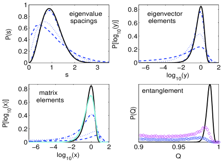
Figure 1: (Color online) Distributions of nearest neighbor eigenvalue spacings (upper-left) and eigenvector element amplitudes (upper-right) for matrices of the interpolating ensembles with $\delta=.1$ (dashed), .5 (dotted) and .9 (chained). The $N=256$ matrix element plot (lower-left) includes the distribution for $\delta=.98$ (light solid line). For this $\delta$ the eigenvalue and eigenvector distributions are indistinguishable from random (solid line) for the resolution of the figure. The matrix element distribution appears to converge more slowly which may be manifest in the entanglement generated by operating with 100 8-qubit $\delta=.9$ ($\bigcirc$), and $.98$ ($\diamond$) matrices on all computational basis states (lower right).

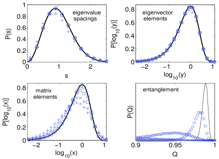
Figure 2: (Color online) Distribution of nearest neighbor eigenvalue spacings (top left), eigenvector elements (top right), matrix elements (bottom left), and $Q$ (bottom right) for $N=256$ pseudo-random maps of $m=2$ (+), 4 ($\times$), 8 ($\square$), and 16 ($\bigcirc$). The eigenvalue and eigenvector distributions appear to converge to that of CUE (solid lines) more quickly than the matrix element distribution and entanglement distribution. To approach $P_{CUE}(Q)$ with one iteration of a map requires $m\simeq 40$ RM ; YSW .

First, we show that the eigenvalue spectrum alone cannot be the sole cause of entanglement generation. This is done in two ways: by identifying a set of operators that have eigenvalues with statistical properties that match CUE but generate no entanglement, and, second, by identifying operators that do not have CUE eigenvalue properties but nevertheless generate CUE levels of entanglement. The first set is that of diagonal operators in which the elements are the eigenvalues of a CUE operator. When applying diagonal operators to computational basis states no entanglement is generated. The eigenvector element distribution and matrix element distribution for these diagonal operators clearly do not follow the CUE distributions. Nevertheless, the eigenvalue spectra fulfill all statistical properties of CUE including nearest-neighbor spacings and higher order correlation functions. The second set of operators are created as follows: let $D$ be a unitary diagonal operator with random phases drawn uniformly from 0 to $2\pi$. Operators $U=U_{CUE}DU_{CUE}^{{\dagger}}$ have eigenvector distributions that follow CUE, matrix element distributions that follow CUE, and entanglement generation equal to CUE. Yet, the nearest-neighbor eigenvalue distribution follows a Poissonian and not the Wigner-Dyson distribution Wigner ; Dyson . What we see from these types of operators is that the eigenvalue distribution of an operator is not a primary factor in an operators’ entanglement generation. This is not to say that operators with high entanglement generation never follow the Wigner-Dyson distribution, as we will see they usually do. Rather, the eigenvalue distribution is not the defining property generating entanglement.

The next step is to divorce the matrix element distribution and entanglement generation of an operator from its eigenvector distribution. This cannot be done completely. Ref. DK proves that the entanglement of the eigenvectors generally provides a lower bound for the asymptotic time value of entanglement generation. This proof is done for bipartite entanglement and can be extended to our investigations because $Q$ is merely the average of bipartite entanglement between each individual qubit and the rest of the system. This bound, however, does not exclude the possibility of a high entanglement generation for operators without random eigenvectors. Nor does this result tell how long it takes to reach this asymptotic value, a necessary question when trying to create a highly entangled state on a quantum computer. Through the use of the interpolating ensembles discussed above we show how the matrix element distribution of an operator relates to these issues.

As mentioned, many of the statistical properties of interpolating ensemble matrices are only weakly dependent on $N$. However, the matrix element distribution and the entanglement generation are strongly dependent on $N$. Fig. 3 shows the eigenvector element distributions and matrix element distributions for $\delta=.9$ interpolating operators at various values of $N$. As $N$ decreases the matrix element distributions approach the CUE distribution. The eigenvector elements on the other hand, are practically constant with $N$.

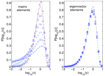
Figure 3: (Color online) Matrix element distribution (left) and eigenvector element distribution (right) for interpolating ensemble matrices with $\delta=.9$ and $N=256$ ($\times$), 128 ($\bigcirc$), 64 ($+$), 32 ($\square$), 16 ($\diamond$), and 8 ($\triangle$). The matrix element distributions gets further and further from that expected of CUE (dashed line for the $N\rightarrow\infty$ limit and chained line for $N=8$) as $N$ increases. This is in contrast with the eigenvector element distribution in which is remarkably stable as a function of $N$.

The average entanglement generated in one iteration of the operator, compared to that expected from CUE matrices, is shown in Fig. 4 as a function of $N$ for the same $\delta=.9$ operators. As $N$ gets smaller the average entanglement generated approaches that of CUE, in a way similar to the matrix element distribution. This despite the fact that the eigenvector element distribution remains constant as a function of $N$. For large $\delta$ interpolating ensemble, say $\delta=.99$, the eigenvector and eigenvalue distributions will be practically indistinguishable from CUE. However, as we see here, the matrix element distribution, and thus the entanglement generation, will fall short of CUE. The larger the Hilbert space the further from CUE. The interpolating ensemble operators thus provide some divergence between the eigenvector distribution and the matrix element distribution. For small $N$ the matrix element distribution and entanglement generation are practically random though the eigenvector element distribution is not. For large $N$ and large $\delta$ the eigenvector element distribution is practically random but the matrix element distribution and entanglement generation are not. This further demonstrates the importance of an operators’ matrix elements in entanglement generation. The time evolution of these operators is explored below.

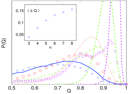
Figure 4: (Color online) Entanglement spectra for CUE operators (lines) and $\delta=.9$ interpolating ensemble operators (shapes), for $N=8$ (solid line and $\times$), 16 (dotted line and $\bigcirc$), 32 (chained line and +) and 64 (dashed line and $\square$). As $N$ increases the distributions of the interpolating ensemble operators diverges further from the CUE distribution. The inset shows the difference between average entanglement generation for CUE operators and the $\delta=.9$ interpolating ensemble operators, $\Delta Q$, as a function of number of qubits, $n=log_{2}(N)$. As $N$ increases the average entanglement production gets further from the CUE average.

A quantum computer programmer starting with a computational basis state and attempting to generate a random state of high multi-partite entanglement will want to apply an operator with a matrix element distribution as close as possible to CUE. Most likely the operator will also exhibit other statistical properties close to CUE, as occurs with pseudo-random operators YSW , but that need not be the case.

Identifying one statistical property that is the dominant cause of high entanglement generation is also important for understanding entanglement as a quantum phenomenon and its relation to quantum chaos. Quantum chaotic operators are known to exhibit many properties of random matrices BGS ; Haake including the ability to produce entanglement. Numerical simulations of two coupled subsystems demonstrate the greater entanglement generation of chaotic versus regular quantum dynamics L1 ; FNP ; MS ; WGSH and analytical results have been obtained through various methods TFM ; L2 ; J . As with the previous classes of operators, we are interested in a quantum chaotic operator’s ability to produce highly entangled states from initial computational basis states. Applying a chaotic operator once will not, in general, produce entanglement on par with random operators Scott ; WGSH . This is in line with the deviant short time behavior of chaotic systems with respect to other statistical properties such as the level or number variance. The deviant behavior is attributed to short periodic phase space orbits AS . Long time entanglement generation behavior is related to the operator’s eigenvectors DK . We have already demonstrated that the operator eigenvalues and eigenvectors are not primary with respect to entanglement generation, thus we demonstrate the observed short and long time entanglement generation behavior is also reflected in the matrix element distribution.

Upon increasing the number of iterations, $t$, of a quantum chaotic operator the average entanglement of initial computational basis states, $\langle Q(t)\rangle$, can approach that of random operators. Similarly, the matrix element distribution of chaotic operators at higher powers approaches the CUE distribution. To demonstrate this we revisit the entanglement production of the BV quantum baker’s map Scott and explore other quantized chaotic maps.

Initial computational basis states evolved under the quantum baker’s map attain $\langle Q\rangle$ values close to $\langle Q_{CUE}\rangle$ only at large $t$ Scott . This is understood based on the baker’s map matrix element distrubtion which does not at all resemble $P_{CUE}(x)$, Fig. 5C. However, for $t=100$ the distribution is much closer to the CUE distribution. For an 8 qubit map $\langle Q(t=1)\rangle$ is only .3080, compared to $\langle Q_{CUE}\rangle=.9883$, while $\langle Q(t=100)\rangle$ is .9597. It is important to note that the quantum baker’s map for Hilbert space dimensions which are a power of 2 is known to have an almost Poissonian nearest neighbor eigenvalue spectrum BV ; sar . Thus, at long times we see relatively high entanglement generation without the presence of a Wigner-Dyson distribution. Rather, more iterations lead to increased matrix element randomness causing the greater entanglement generation.

We study two other examples of quantized chaotic maps: the quantum sawtooth map saw1 ; saw2 ,

$$U_{saw}=\frac{e^{-i\pi/4}}{\sqrt{N}}e^{ik\pi m^{2}/N}e^{i\pi(n-m)^{2}/N},$$ (7)

and the quantum Harper map harper ,

$$U_{H}=e^{iN\gamma\cos(2\pi q/N)}e^{iN\gamma\cos(2\pi p/N)}.$$ (8)

All elements of the chaotic, $k=1.5$, and regular, $k=-1.5$, sawtooth maps have equal amplitude. One iteration of either map on any computational basis state yields a state with $Q=1$. For the chaotic sawtooth, the matrix element randomness increases with $t$, such that at $t=50$ the matrix element distribution is practically $P_{CUE}(x)$ and $\langle Q(t=50)\rangle=.98826$. For the regular sawtooth $\langle Q\rangle$ oscillates wildly as seen in figure 5. This stems from the lack of an asymptotic randomness for the matrix elements.

The matrix elements for the chaotic Harper, $\gamma=1$, deviate only slightly from $P_{CUE}(x)$, and $\langle Q(t=1)\rangle=.9814$. For $t=50$ there is an increase in matrix element randomness and $\langle Q(t=50)\rangle=.9882$. The regular Harper map, $\gamma=.1$, matrix element distribution and $\langle Q\rangle$ also approach asymptotic limits as $t$ increases. These limits fall short of the random matrix statistics but the average entanglement is still $\langle Q(t\rightarrow\infty)\rangle\simeq.95$. Note that the asymptotic average entanglement of the regular Harper is about the same as that of the baker’s map. In addition, the average entanglement after one iteration of the map is higher for the regular Harper than for the baker’s map. This appears to be an exception to the conjecture that entanglement is a signature of quantum chaos. The quantum baker’s map is widely considered chaotic since it is the quantum analog of a chaotic map. The Harper’s map for $k=-1.5$ is not chaotic since it is the quantum analog of a regular map. Yet the entangling power of the Harper’s map appears to be at least as good, if not better, than that of the baker’s map.

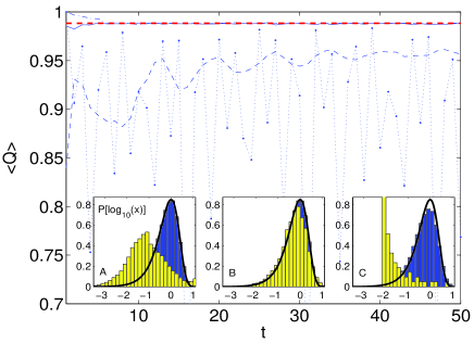
Figure 5: (Color online) Average entanglement, $\langle Q\rangle$, over all 8-qubit initial computational basis states as a function of time for quantum sawtooth maps, $k=1.5$ (chained line) and $k=-1.5$ (dotted line), and Harper maps, $\gamma=1$ (solid line) and $\gamma=.1$ (dashed line), compared to the random matrix average (horizontal dashed line). The chaotic maps quickly approach the random matrix average while the regular maps do not. The insets show matrix element distributions for the regular (light) and chaotic (dark) sawtooth maps at $t=50$ (A), the regular (light) and chaotic (dark) Harper maps at $t=50$ (B), and $t=1$ (light) and 100 (dark) of the baker’s map (C).

Finally, we return to the interpolating ensembles matrix element distribution and $\langle Q\rangle$ now as a function of time. As shown in DK we expect that the entanglement will approach the entanglement of the eigenvectors. However, we show here how matrix elements affect this and how operators with similar matrix element distributions lead to similar average entanglement generation. Fig. 6 shows $\langle Q(t)\rangle$ for $\delta=.9$ ($\times$), and .98 ($\bigcirc$) operators, already explored in YSW , and the matrix element distribution at the same points in time. As the number of iterations increase the entanglement production exponentially approaches the CUE value (dashed line). The matrix element distribution also converges to the CUE distribution. Comparing the entanglement produced by these operators we note that $\langle Q(t=5,10,15,20,30)\rangle$ of the $\delta=.9$ operators equal $\langle Q(t=1,2,3,4,6)\rangle$, respectively, of the $\delta=.98$ operators. The matrix element distributions producing these entanglement values are practically equal.

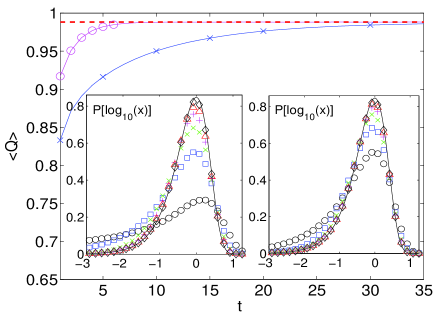
Figure 6: (Color online) Average entanglement generation as a function of time for 50 interpolating ensemble operators with $\delta=.9$ ($\times$), and .98 ($\bigcirc$) operators on initial computational basis states. For both sets of operators the average entanglement produced approaches the CUE average (dashed line) as an exponential. The insets show the matrix element distributions for the same set of operators as a function of time. The left inset shows the distribution for $\delta=.9$ operators for $t=1(\bigcirc)$, 5 ($\square$), 10 ($\times$), 15 (+), 20 ($\triangle$), and 30 ($\diamond$). The right inset shows the matrix element distributions for $\delta=.98$ operators and $t=1(\bigcirc)$, 2 ($\square$), 3 ($\times$), 4 (+), 5 ($\triangle$), and 6 ($\diamond$). Both sets of operators matrix element distributions approach CUE as time increases.

In conclusion, we have explored the connection between an operators matrix element distribution and its multi-partite entangling power on initial computational basis states. We have shown that operators with CUE distributions of eigenvalues and eigenvectors are not the sole cause of CUE-like entangling power. CUE-like entangling power cannot be achieved without a CUE distribution of matrix elements. In addition, operators without CUE distributions of eigenvalues and eigenvectors can still have CUE-like entangling power if the operators have a random matrix element distribution. It also appears that operators with similar matrix element distributions generate similar amounts of entanglement. This analysis should provide a more specified goal in the search for efficient means of random state production.

The authors thank K. Zyczkowski for clarifying interpolating ensemble generation and helpful discussions. The authors acknowledge support from the DARPA QuIST (MIPR 02 N699-00) program. YSW acknowledges support of the National Research Council through the Naval Research Laboratory. Computations were performed at the ASC DoD Major Shared Resource Center.

Appendix A Appendix A

CUE construction based on the Hurwitz parameterization starts with elementary unitary transformations, $E^{(i,j)}(\phi,\psi,\chi)$, with non-zero elements Zyc2

$$E_{kk}^{(i,j)} = 1,\;\;\;\;k=1,...,N,\;\;\;\;k\neq i,j$$

$$E_{ii}^{(i,j)} = e^{i\psi}\cos\phi,\;\;\;\;\;\;\;\;\;E_{ij}^{(i,j)}=e^{i\chi}\sin\phi$$

$$E_{ji}^{(i,j)} = -e^{-i\chi}\sin\phi,\;\;\;\;E_{jj}^{(i,j)}=e^{-i\psi}\cos\phi$$ (9)

which are used to form $N-1$ composite rotations

$$E_{1} = E^{(N-1,N)}(\phi_{01},\psi_{01},\chi_{1})$$

$$E_{2} = E^{(N-2,N-1)}(\phi_{12},\psi_{12},0)E^{(N-1,N)}(\phi_{02},\psi_{02},\chi_{2})$$

$$\dots$$

$$E_{N-1} = E^{(1,2)}(\phi_{N-2,N-1},\psi_{N-2,N-1},0)\times$$ (10)

$$E^{(2,3)}(\phi_{N-3,N-1},\psi_{N-3,N-1},0)\times$$

$$\dots E^{(N-1,N)}(\phi_{0,N-1},\psi_{0,N-1},\chi_{N-1}).$$

A CUE matrix is finally attained by $U_{CUE}=e^{i\alpha}E_{1}E_{2}\dots E_{N-1}$. The Euler angles $\psi$, $\chi$, and $\alpha$ are drawn uniformly from the intervals

$$0\leq\psi_{rs}\leq 2\pi,\;\;\;\;\;\;0\leq\chi_{s}\leq 2\pi,\;\;\;\;\;\;0\leq\alpha\leq 2\pi,$$ (11)

and $\phi_{rs}=\sin^{-1}({\xi_{rs}}^{1/(2r+2)})$, with $\xi_{rs}$ drawn uniformly from 0 to 1. The $2\times 2$ block $E^{(i,j)}_{m,n}$ with $m,n=i,j$ and $r=0$ is a random SU(2) rotation with respect to the Haar measure. The interpolating ensembles Zyc3 follow the same construction but the angles are drawn from constricted intervals

$$0\leq\psi_{rs}\leq 2\pi\delta,\;\;\;\;\;\;0\leq\chi_{s}\leq 2\pi\delta,\;\;\;\;\;\;0\leq\alpha\leq 2\pi\delta,$$ (12)

with $\phi_{rs}=\sin^{-1}(\delta{\xi_{rs}}^{1/(2r+2)})$ and $\xi_{rs}$ drawn from 0 to 1. The whole is multiplied by a diagonal matrix of random phases drawn uniformly from 0 to $2\pi$. The parameter $\delta$ ranges from 0 to 1 and provides a smooth transition of certain statistical properties between the diagonal circular Poisson ensemble (CPE) and CUE Zyc3 .

References

- (1) A. Scott and C. Caves, J. Phys. A, 36, 9553, (2003).
- (2) A. Harrow, P. Hayden, and D. Leung, Phys. Rev. Lett. 92, 187901 (2004).
- (3) C.H. Bennett, P. Hayden, D. Leung, P. Shor, and A. Winter, quant-ph/0307100.
- (4) P. Hayden, D. Leung, P. Shor, and A. Winter, Commun. Math. Phys. 250, 371, (2004).
- (5) X. Wang, S. Ghose, B.C. Sanders, and B. Hu, Phys. Rev. E, 70, 016217, (2004).
- (6) J. Emerson, Y.S. Weinstein, M. Saraceno, S. Lloyd, and D.G. Cory, Science, 302, 2098, (2003).
- (7) Y.S. Weinstein and C.S. Hellberg, Phys. Rev. A, 69, 062301, (2004).
- (8) Y.S. Weinstein and C.S. Hellberg, Phys. Rev. A, 71, 014303, (2005).
- (9) Y.S. Weinstein and C.S. Hellberg, to be published, Phys. Rev. Lett., quant-ph/0502110.
- (10) K. Zyczkowski and M. Kus, Phys. Rev. E, 53, 319, (1996).
- (11) O. Bohigas, M.J. Giannoni, and C. Schmit, Phys. Rev. Lett., 52, 1, (1984).
- (12) K. Zyczkowski and M. Kus, J. Phys. A, 27, 4235, (1994); M. Pozniak, K. Zyczkowski, and M. Kus, J. Phys. A, 31, 1059, (1998).
- (13) F. Haake and K. Zyczkowski, Phys. Rev. A, 42, R1013, (1990).
- (14) D.A. Meyer and N.R. Wallach, J. Math. Phys., 43, 4273, (2002).
- (15) G.K. Brennen, Quant. Inf. Comp., 3, 619, (2003).
- (16) K. Zyczkowski, Phys. Rev. E, 56, 2257 (1997).
- (17) H. Schomerus and C.W.J. Beenakker, Phys. Rev. Lett. 84, 3927 (2000).
- (18) J.N.H.J. Cremers and P.W. Brouwer, Phys. Rev. B, 65, 115333 (2002).
- (19) E.P. Wigner, Ann. Math. 62, 548 (1955); 65, 203 (1957).
- (20) F.J. Dyson, J. Math. Phys. 3, 140, (1962);
- (21) R. Demkowicz-Dobrzanski and M. Kus, Phys. Rev. E, 70, 066216, (2004).
- (22) F. Haake, Quantum Signatures of Chaos, (Springer, New York, 1992).
- (23) A. Lakshminarayan, Phys. Rev. E, 64, 036207, (2001); J.N. Bandyopadhyay and A. Lakshminarayan, Phys. Rev. Lett., 89, 060402, (2002).
- (24) K. Furuya, M.C. Nemes, and G.Q. Pellegrino, Phys. Rev. Lett., 80, 5524, (1998).
- (25) P.A. Miller and S. Sarkar, Phys. Rev. E, 60, 1542 (1999).
- (26) A. Tanaka, H. Fujisaki, and T. Miyadera, Phys. Rev. E, 66, 045201(R), (2002); H. Fujisaki, T. Miyadera, and A. Tanaka, Phys. Rev. E, 67, 066201, (2003).
- (27) J.N. Bandyopadhyay and A. Lakshminarayan, Phys. Rev. E, 69, 016201, (2004).
- (28) Ph. Jacquod, Phys. Rev. Lett., 92, 150403, (2004).
- (29) R. Aurich, F. Steiner, Physica D, 82, 266 (1994).
- (30) N. L. Balazs and A. Voros, Ann. Phys., 190, (1989).
- (31) M. Saraceno, Ann. Phys. 199, 37 (1990).
- (32) A. Lakshminarayan and N.L. Balzs, Chaos Soliton Fract., 5, 1169, (1995).
- (33) G. Benenti, G. Casati, S. Montangero, and D.L. Shepelyansky, Phys. Rev. Lett., 87, 227901, (2001).
- (34) P. Leboeuf, J. Kurchan, M. Feingold, and D.P. Arovas, Phys. Rev. Lett., 65, 3076, (1990).