Non-destructive Orthonormal State Discrimination

Abstract

We provide explicit quantum circuits for the non-destructive deterministic discrimination of Bell states in the Hilbert space $C^{d^{n}}$, where $d$ is qudit dimension. We discuss a method for generalizing this to non-destructive measurements on any set of orthogonal states distributed among $n$ parties. From the practical viewpoint, we show that such non-destructive measurements can help lower quantum communication complexity under certain conditions.

I Introduction

Entangled states play a key role in the transmission and processing of quantum information Niel ; suter . Using an entanglement channel, an unknown state can be teleported bouw with local unitary operations, appropriate measurement and classical communication; one can achieve entanglement swapping through joint measurement on two entangled pairs pan1 . Entanglement leads to increase in the capacity of the quantum information channel, known as quantum dense coding Mattle . The bipartite, maximally entangled Bell states provide the most transparent illustration of these aspects, although three particle entangled states like GHZ and W states are beginning to be employed for various purposes carvalho ; hein .

Making use of single qubit operations and the C-NOT gates, one can produce various entangled states in a quantum network Niel . It may be of interest to know the type of entangled state that is present in a quantum network, at various stages of quantum computation and cryptographic operations, without disturbing these states. Nonorthogonal states cannot be discriminated with certainty wootters , while the discrimination of orthogonal states are possible. A large number of results regarding distinguishing various orthogonal states, have recently been established walgate ; gosh1 ; vermani ; chen . If two copies belonging to the four orthogonal Bell states are provided, local operations and classical communication (LOCC) can be used to distinguish them with certainty. It is not possible to discriminate using only LOCC, either deterministically or probabilistically among the four Bell states, if only a single copy is provided gosh1 . It is also not possible to discriminate multipartite orthogonal states by using LOCC only gosh2 . However, any two multipartite orthogonal states can be unequivocally distinguished through LOCC walgate .

A number of theoretical and experimental results already exist in this area of unambiguous state discrimination cola ; pan2 ; kim . Appropriate unitary transforms and measurements, which transfer the Bell states into disentangled basis states, can unambiguously identify all the four Bell states pan2 ; kim ; boschi . However, in the process of measurement the entangled state is destroyed. Of course, the above is satisfactory when the Bell state is not required further in the quantum network.

We consider in this work the problem of discriminating a complete set of orthogonal basis states in $C^{d^{n}}$– of which the conventional Bell states form a special case– where the $n$ qudits ($d$-level systems) are distributed among $n$ players. We present a scheme which deterministically discriminates between these states without vandalizing them, such that these are preserved for further use. This article is divided as follows. In Section II, we present circuits for the non-destructive Bell state discrimination for $n$ qubits shared among $n$ players, beginning with the case of conventional Bell states. In Section III, this result is generalized to construct circuits for Bell state discrimination among qudits. In Section IV, we point out the underlying mathematical structure that clarifies how our proposed circuits work. In principle, this can be used to further generalize our results of Section III to discrimination of any set of orthogonal states. In Section V, we examine specific situations where such non-destructive measurements can be useful in computing and cryptography. An appendix is attached at the end, which shows closure property of generalized Bell states, used in the text under Hadamard operations.

II Bell state discrimination in $C^{2^{n}}$ Hilbert space

In principle, any set of orthogonal states can be discriminated in quantum mechanics, but LOCC may not be sufficient if the state is distributed among two or more players. Here we start with a $C^{2^{n}}$ Hilbert space. To describe any state in this Hilbert space we need $2^{n}$ orthonormal basis vectors. The choice of the basis is not unique, but one choice of particular importance is the set of maximally entangled $n$-qubit generalization of Bell states given by:

$$|\psi_{x}^{+}\rangle = \frac{1}{\sqrt{2}}(|x\rangle+|\bar{x}\rangle),$$ (1a)

$$|\psi_{x}^{-}\rangle = \frac{1}{\sqrt{2}}(|x\rangle-|\bar{x}\rangle)$$ (1b)

where $x$ varies from 0 to $2^{n-1}-1$ and $\bar{x}\equiv 1^{\otimes n}\oplus x$ in modulo 2 arithmetic. The set of complete basis vectors (1) reduces to Bell basis for $n=2$ and to GHZ states for $n=3$. As an example, setting $n=2$ in (1) we get the usual Bell states

$$|\psi_{00}\rangle=|\psi^{+}\rangle = \frac{1}{\sqrt{2}}(|00\rangle+|11\rangle),$$

$$|\psi_{01}\rangle=|\phi^{+}\rangle = \frac{1}{\sqrt{2}}(|01\rangle+|10\rangle),$$

$$|\psi_{10}\rangle=|\psi^{-}\rangle = \frac{1}{\sqrt{2}}(|00\rangle-|11\rangle),$$

$$|\psi_{11}\rangle=|\phi^{-}\rangle = \frac{1}{\sqrt{2}}(|01\rangle-|10\rangle).$$ (2)

A circuit to non-destructively discriminate the generalized orthonormal entangled basis states (1) employing ancilla is shown in Fig. 1. To discriminate the members of the entangled, orthonormal basis set in $C^{2^{n}}$, we have to communicate and carry out measurements on $n$ ancillary qubits in the computational basis. The first measurement is done on the state $|R_{nA_{1}}\rangle$, as shown in Eq. (3a). This measurement determines the relative phase between $|x\rangle$ and $|\bar{x}\rangle$. It will give $0$ for $\frac{1}{\sqrt{2}}(|x\rangle+|\bar{x}\rangle)$ and $1$ for $\frac{1}{\sqrt{2}}(|x\rangle-|\bar{x}\rangle)$. The next measurements compare the parity between two consecutive bits and yield zero if the bits coincide and one, otherwise. This follows from Eq. (3b), which shows the state for the complex of the system and the $i$th ancilla, where $2\leq i\leq n$. Each ancilla $A_{i}$ is sequentially interacted with the system and then measured. It can be shown (Section III) that this action leaves the states $|\psi^{\pm}_{x}\rangle$ undisturbed. This means that the corresponding measurements, $M_{i}$, represent commuting observables. In general, $M_{1}$ gives the phase bit, and $M_{i}$ gives the parity of the string comprising of the $i$th and $i{+}1$th qubits.

In a way clarified in Section IV, $M_{1}$ may be regarded as the non-destructive equivalent of measuring $X^{\otimes n}$ and $M_{i}$ ($2\leq i\leq n$) that of measuring $Z\otimes Z$, so that the simultaneous measurability of any pair of $M_{i}$’s follows from the fact that $[X^{\otimes n},Z(j)\otimes Z(k)]=0$ and $[Z(j)\otimes Z(k),Z(j^{\prime})\otimes Z(k^{\prime})]=0$ where $Z(j)$ is the Pauli $Z$ operator acting on the $j$th qubit.

A note on notation: the sign $Q(j\leftarrow k)$ signifies a C-NOT gate, with $k$ being (ancilla) control index number, and $j$ being (system) target index number. Conversely, $Q(j\rightarrow k)$ signifies a C-NOT gate with $j$ being (system) control index number and $k$ being (ancilla) target index number.

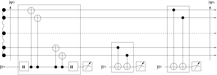
Figure 1: Diagram depicting the circuit for non-destructive generalized orthonormal qubit Bell state discriminator. The first bounded box depicts, in a sense clarified in Section IV, an effective, non-destructive measurement of $X^{\otimes n}$, which yields the phase bit value. The second and third boxes depict an effective, non-destructive measurement of $Z^{{\dagger}}\otimes Z$, which yields the relative parity between two consecutive qubits. To obtain the full relative parity information, $n-1$ relative parity measurements are required.

$$|R_{(n\times 2)A1}\rangle = \left[I_{2}^{\otimes n}\otimes H_{2}\right]\times\left[\bigotimes_{j=1}^{n}Q(j\leftarrow 1)\right]\times\left[I_{2}^{\otimes n}\otimes H_{2}\right](|\Psi\rangle_{1\cdots n}\otimes|0\rangle_{A1}),$$ (3a)

$$|R_{(n\times 2)Ai}\rangle = \left[Q([i-1]\rightarrow i)\otimes Q\left([{i}\rightarrow{i}\right)\right]\left(|\Psi\rangle_{1\cdots n}\otimes|0\rangle_{Ai}\right),$$ (3b)

where $2\leq i\leq n-1$. Therefore, all together we need $n$ measurements on $n$ ancillary qubits to discriminate $2^{n}$ orthonormal, entangled basis states of the form (1). Furthermore, we require $3n-2$ applications of CNOT gates. The question of quantity of quantum communication required, which depends on the topology of the quantum communication network, is discussed in Section V in detail.

A proof that the circuit described in Eq. (3), and depicted in Fig. 1 achieves the required Bell state discrimination is deferred to Section III. Here we simply illustrate it using the specific example of the usual Bell states (2). Since (1) reduces to (2) for $n=2$, our generalized circuit reduces to that shown in Fig. 2, where one needs only two ancillary qubits, four CNOT gates, two measurements and two qubits of quantum communication.

In Table 1, we have shown the results of the measurements on both the ancillas when different Bell states are present in the given circuit (Fig. 2). Just before measurement, the states can be explicitly written as,

$$|R_{(2\times 2)A1}\rangle = \left[I_{2}\otimes I_{2}\otimes H_{2}\right]\times[Q(1\leftarrow 1)\otimes Q(2\leftarrow 1)]\times\left[I_{2}\otimes I_{2}\otimes H_{2}\right](|\Psi\rangle_{12}\otimes|0\rangle_{A1})$$ (4a)

$$|R_{(2\times 2)A2}\rangle = \left[Q(1\rightarrow 2)\otimes Q(2\rightarrow 2)\right]\left(|\Psi\rangle_{12}\otimes|0\rangle_{A2}\right).$$ (4b)

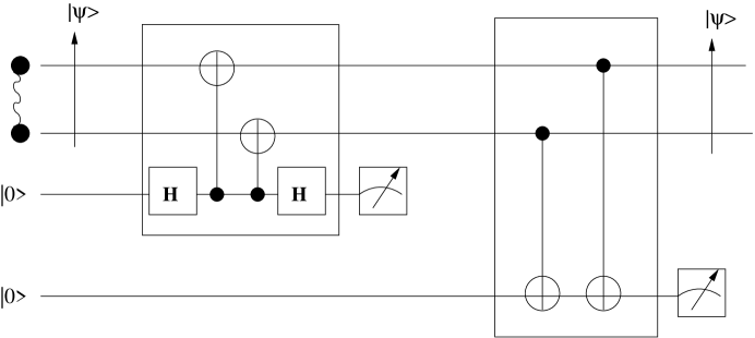
Figure 2: A special case of Fig. 1: the diagram depicting the circuit for Bell state discriminator.

Bell State	Measurement $A_{1}$	Measurement $A_{2}$
$|\psi^{+}\rangle$	$0$	$0$
$|\psi^{-}\rangle$	$1$	$0$
$|\phi^{+}\rangle$	$0$	$1$
$|\phi^{-}\rangle$	$1$	$1$

Table 1: Results of outsourced measurements on two ancilla for the Bell states 2

.

Thus we have provided a circuit for orthonormal qubit Bell state discrimination shared between two or more parties. These results can be straightforwardly generalized, as shown in the following Section.

III Generalized Bell state discrimination in $\mathbb{C}^{d^{n}}$

The results of the preceding Section can be generalized to entangled states of $n$ qudits. To this end, we replace the regular Pauli matrices with their $d$-dimensional analogs kni96 . We generalize $X$ and $Z$ gates; these denoted by $X_{d}$ and $Z_{d}$, respectively, have the action:

$$Z_{d}|j\rangle \mapsto e^{2\pi\iota j/d}|j\rangle$$ (5a)

$$X_{d}|j\rangle \mapsto |j-1\rangle,$$ (5b)

where the increment in the ket is in mod $d$ arithmetic. The operators $X_{d}$ and $Z_{d}$ are related by a Fourier transform $X_{d}=H_{d}Z_{d}H_{d}^{{\dagger}}$, where $H_{d}$ is the generalized Hadamard transformation given by:

$$(H_{d})_{jk}=\frac{1}{\sqrt{d}}e^{2\pi\iota j\cdot k/d}.$$ (6)

Unlike the qubit case, $Z_{d},X_{d}$ and $H_{d}$ are not Hermitian.

The $d$ generalized Bell states are

$$|\Psi_{pq}\rangle=\frac{1}{\sqrt{d}}\sum_{j}e^{2\pi\iota jp/d}|j\rangle|j+q\rangle,\hskip 28.45274pt(0\leq p,q\leq d-1)$$ (7)

which form an orthogonal, complete basis of maximally entangled vectors for the $d^{2}$ dimensional ”qudit” space ben93 . The parameter $p$ denotes phase and $q$ the generalized parity. The states $|\Psi_{pq}\rangle$ are $d$-dimensional analogs of Bell states (2) in that they are eigenstates of the operator $X_{d}\otimes X_{d}$, which is equivalent to the phase observable, whose eigenvalues are $p$ or some function $f(p)$, and $Z_{d}^{{\dagger}}\otimes Z_{d}$, which is equivalent to the parity observable, whose eigenvalues are $q$ or some real-valued function $f(q)$. Therefore, measurements equivalent to these operators guarantee a complete characterization of the generalized Bell states. Furthermore, the set of generalized Bell states remains closed under the action $H^{{\dagger}}_{d}\otimes H$ or $H_{d}\otimes H_{d}^{{\dagger}}$ or (cf. Appendix A).

The generalization of the CNOT that we require is the one, whose action we define by,

$${\cal C}_{X}:|j\rangle|k\rangle\longmapsto|j\rangle|j-k\rangle.$$ (8)

The reason for this choice is clarified in Section IV. We use the following notation: the sign ${\cal C}_{X}(j\leftarrow k$) signifies a C-SUM gate with $k$ being (ancilla) control index number, and $j$ being (system) target index number; ${\cal C}_{X}(j\rightarrow k$) signifies a C-SUM gate with the control-target order reversed. A similar terminology extends to the two-qudit gate ${\cal C}_{X}^{{\dagger}}$, whose action is given by either $|j\rangle|k\rangle\longmapsto|j\rangle|k-j\rangle$ or $|j\rangle|k\rangle\longmapsto|j-k\rangle|j\rangle$, depending on whether the system or ancilla is the control register.

A direct generalization to $d$-dimension of Eq. (4) is

$$|R_{(2\times d)A1}\rangle = [I_{d}\otimes I_{d}\otimes H_{d}]\times\left[{\cal C}_{X}(1\leftarrow 1){\cal C}_{X}(2\leftarrow 1)\right]\times[I_{d}\otimes I_{d}\otimes H_{d}^{\dagger}](|\Psi\rangle_{12}\otimes|0\rangle_{A1}).$$ (9a)

$$|R_{(2\times d)A2}\rangle = \left[{\cal C}_{X}(1\rightarrow 2){\cal C}_{X}^{{\dagger}}(2\rightarrow 2)\right](|\Psi\rangle_{12}\otimes|0\rangle_{A2}).$$ (9b)

We will denote the observables corresponding to circuits (9a) and (9b) as $M_{1}$ and $M_{2}$, respectively. $M_{1}$ will yield the ‘phase value’ $p$, and $M_{2}$ the generalized parity, $q$. In a way clarified in Section IV, $M_{1}$ and $M_{2}$ correspond, respectively, to the unitary operations $X\otimes X$ and $Z^{{\dagger}}\otimes Z$, so that the simultaneous measurability of $M_{1}$ and $M_{2}$ can be shown as a consequence of the fact that $[X\otimes X,Z^{{\dagger}}\otimes Z]=0$. More directly, we will show that both measurements leave the state $|\Psi_{pq}\rangle$ undisturbed.

Let us now consider the more general system of $n$ qudits. The elements of the $d^{n}$ dimensional vector space over the modulo $d$ field is given by the set $V_{d}^{\times n}\equiv\{{\bf x}_{j}=(x_{1},x_{2},\cdots,x_{n})\}$. Consider the equivalence relation given by ${\bf x}_{j}\equiv{\bf x}_{k}$ if and only if ${\bf x}_{j}-{\bf y}_{k}$ is a uniform vector, i.e., one of the form $(r,r,r,\cdots,r)$, where $r\in\{0,1,2,\cdots,d-1\}$. There are $d^{n-1}$ equivalence classes, uniquely labeled by the coordinates $(q_{1},q_{2},\cdots,q_{n-1})\in V_{d}^{\times(n-1)}$. A complete, maximally entangled Bell basis for the Hilbert space $\mathbb{C}^{d^{n}}$ can be given by:

$$|\Psi_{pq_{1}q_{2}\cdots q_{n-1}}\rangle=\sum_{j=0}^{d-1}e^{2\pi\iota j\cdot p/d}|j,q_{1}+j,q_{2}+j,\cdots,q_{n-1}+j\rangle.$$ (10)

We call them Bell states in the sense that any state $|\Psi_{pq_{1}q_{2}\cdots q_{n-1}}\rangle$ is an eigenstate of $X_{d}^{\otimes n}$ and $Z_{d}(j)\otimes Z_{d}^{{\dagger}}(j+1)$ ($1\leq j\leq(n-1)$), which, in a way clarified in Section IV, correspond to observables with eigenvalues $p$ and $q_{j+1}-q_{j}$ respectively, the latter being called the relative parity.

A generalization of Eq. (9) to $n$ qudits is Eq. (11), which describes a circuit to measure phase information $p$ and generalized parity information $q_{1},q_{2},\cdots,q_{n-1}$ of such states. The circuit is depicted in Fig. 3.

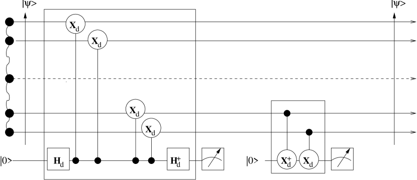
Figure 3: Diagram depicting the circuit for non-destructive generalized orthonormal qudit Bell state discriminator. The first bounded box depicts the outsourced measurement of an observable that is compatible with $X_{d}^{\otimes n}$, which for the generalized Bell states yields the global phase value $p$. The second box depicts the outsourced measurement of an observable compatible with $Z_{d}^{{\dagger}}\otimes Z_{d}$, which yields the relative parity between two consecutive qudits. To obtain the full relative parity information, $n-1$ such relative parity measurements are needed.

The required ancilla are $n$ qudits. The corresponding equation is obtained by generalizing Eqs. (3).

$$|R_{(n\times d)A1}\rangle = \left[I_{d}^{\otimes n}\otimes H_{d}^{{\dagger}}\right]\times\left[\Pi_{j=1}^{n}{\cal C}_{X}(j\leftarrow 1)\right]\times\left[I_{d}^{\otimes n}\otimes H_{d}\right](|\Psi\rangle_{1\cdots n}\otimes|0\rangle_{A1}),$$ (11a)

$$|R_{(n\times d)Ai}\rangle = \left[{\cal C}_{X_{d}}([i-1]\rightarrow i){\cal C}_{X}^{{\dagger}}(i\rightarrow i)\right]\left(|\Psi\rangle_{1\cdots n}\otimes|0\rangle_{Ai}\right).$$ (11b)

We will denote the measurements realized by these circuits, via ancilla $A_{i}$, by $M_{i}$ ($1\leq i\leq n$). To see that the $M_{i}$’s are compatible, and that therefore their actions are non-destructive, it turns out to be sufficient to note that $[X_{d}^{\otimes n},Z_{d}(j)\otimes Z_{d}^{{\dagger}}(k)]=0$ ($j\neq k$) and $[Z_{d}(j)\otimes Z_{d}^{{\dagger}}(k),Z_{d}(j^{\prime})\otimes Z_{d}^{{\dagger}}(k^{\prime})]=0$ ($j\neq k$, $j^{\prime}\neq k^{\prime}$), which indeed follows from the fact the states $|\Psi_{pq_{1}q_{2}\cdots q_{n-1}}\rangle$ are eigenstates of $X_{d}^{\otimes n}$ and $Z_{d}^{{\dagger}}(j)\otimes Z_{d}(k)$. We show below explicitly that the $M_{i}$’s measure $|\Psi_{pq_{1}q_{2}\cdots q_{n-1}}\rangle$ non-destructively.

To see this, we note that the action of the first two (boxed) operations in Eq. 11a on a state $|\Psi_{pq_{1}q_{2}\cdots q_{n-1}}\rangle|k\rangle$ is

$$|\Psi_{pq_{1},q_{2},\cdots,q_{n-1}}\rangle|k\rangle = \left[\sum_{j=0}^{d-1}e^{2\pi\iota j\cdot p/d}|j,q_{1}+j,q_{2}+j,\cdots,q_{n}+j\rangle\right]|k\rangle$$ (12)

$$\longrightarrow \left[\sum_{j=0}^{d-1}e^{2\pi\iota j\cdot p/d}|j,q_{1}+j-k,q_{2}+j-k,\cdots,q_{n}+j-k\rangle\right]|k\rangle$$

$$= \left[\sum_{j^{\prime}=0}^{d-1}e^{2\pi\iota j^{\prime}\cdot p/d}|j^{\prime},q_{1}+j^{\prime},q_{2}+j^{\prime},\cdots,q_{n}+j^{\prime}\rangle\right]|k\rangle$$

$$= e^{2\pi\iota k\cdot p/d}|\Psi_{pq_{1},q_{2},\cdots,q_{n-1}}\rangle|k\rangle,$$

from which it follows that full effect of the operation described in Eq. (11a) produces the state:

$$|\Psi_{pq_{1},q_{2},\cdots,q_{n-1}}\rangle H_{d}|k\rangle = |\Psi_{pq_{1},q_{2},\cdots,q_{n-1}}\rangle\left(\frac{1}{\sqrt{d}}\sum_{j=0}^{d-1}|j\rangle\right)$$ (13)

$$\longrightarrow |\Psi_{pq_{1},q_{2},\cdots,q_{n-1}}\rangle\left(\frac{1}{\sqrt{d}}\sum_{j=0}^{d-1}e^{2\pi\iota p\cdot j/d}|j\rangle\right)$$

$$\longrightarrow |\Psi_{pq_{1},q_{2},\cdots,q_{n-1}}\rangle|p\rangle.$$

This yields the phase bit upon the ancilla being measured.

It is easily seen that the action (11b) non-destructively extracts the relative parity information. For,

$$\left[{\cal C}_{X_{d}}([i-1]\rightarrow i){\cal C}_{X_{d}}^{{\dagger}}(i\rightarrow i)\right]|\Psi_{pq_{1},q_{2},\cdots,q_{n-1}}\rangle|0\rangle_{i}$$ (14)

$$= {\cal C}_{X_{d}}([i-1]\rightarrow i)\sum_{j=0}^{d-1}e^{2\pi\iota j\cdot p/d}|j,q_{1}+j,q_{2}+j,\cdots,q_{n-1}+j\rangle|q_{i+1}+j\rangle_{i}$$

$$= \sum_{j=0}^{d-1}e^{2\pi\iota j\cdot p}|j,q_{1}+j,q_{2}+j,\cdots,q_{n-1}+j\rangle|q_{i+1}-q_{i}\rangle_{i}$$

$$= |\Psi_{pq_{1},q_{2},\cdots,q_{n-1}}\rangle|q_{i+1}-q_{i}\rangle_{i}.$$

The operation $\left[{\cal C}_{X_{d}}([i-1]\rightarrow i){\cal C}_{X_{d}}^{{\dagger}}(i\rightarrow i)\right]$ serves to entangle and then disentangle the input Bell state and the ancilla, such that the relative parity of the two concerned qudits can be read off the latter in the computational basis. This also proves that the circuits given in Eqs. (3), (4) and (9) perform non-destructive Bell state discrimination in dimensions $2^{n}$, $2\times 2$ and $d\times d$, respectively, for they are all special cases of the circuit described in Eq. (11).

Note that although the circuit for qubits in Fig. 1 and for qudits in Fig.3 use relative parity measurements on consecutive pairs of qudits, they need not do so. Given any set of $n-1$ relative parity values $q_{j}-q_{k}$ that suffice to fully determine the $q_{j}$’s in a state $|\Psi_{pq_{1}q_{2}\cdots q_{n-1}}\rangle$, our non-destructive measurements are such that the generalized Bell states are eigenstates of such operators, and hence form a complete set of compatible observables. In Section IV, we show that such relative parity measurements correspond to an observable compatible with $Z^{{\dagger}}_{d}(j)\otimes Z_{d}(k)$ (in the $d=2$ case, the observable is identical with $Z(j)\otimes Z(k)$). Depending on the topology of the quantum communication network available, the choice of relative parity measurements can vary. For example, if the communication network has a star topology, as in Fig. 4(a), then the set of observables can correspond to $Z^{{\dagger}}_{d}(1)\otimes Z_{d}(j)$, where 1 is the hub index (marked $A$ in the figure), and $j$ runs through the remaining vertices. Since any of the operators $X_{d}^{\otimes n}$ and $Z^{{\dagger}}_{d}(j)\otimes Z_{d}(k)$ commute, by corollary 1 (in Section IV) the non-destructive versions of measurements compatible with them can be simultaneously determined.

Figure 4: Two possible configurations of the quantum communication network: (a) In a star topology, a set of ‘relative parity’ measurements could be along each edge; (b) in the linear configuration, the strategy of observing consecutive qubits or qudits, as given in Eqs. (3b) or (9b), can be used.

IV General circuits for non-destructive orthonormal state discrimination

In this Section, we will examine the basic mathematical structure underlying our circuits. In so doing, we will be able to adapt the ideas of the preceding Sections to the case of any orthonormal state discrimination. As pointed out earlier, the generalized Bell states are eigenstates of the unitary operators $X_{d}^{\otimes n}$ and $Z_{d}^{{\dagger}}\otimes Z_{d}$, where $d,n\geq 2$. We mentioned that the non-destructive measurement $M_{1}$, effected through the ancilla $A_{1}$ was equivalent to measuring an observable compatible with the unitary operators $X_{d}^{\otimes n}$, while the non-destructive measurement $M_{i}$ ($2\leq i\leq n$), effected through the ancilla $A_{i}$, was equivalent to measuring an observable compatible with the unitary operators $Z_{d}^{{\dagger}}\otimes Z_{d}$. That is to say, the ancillary measurements are such that $X_{d}^{\otimes n}=\exp(2\pi\iota M_{1}/d)$ and $Z_{d}^{{\dagger}}(i-1)\otimes Z_{d}(i)=\exp(2\pi\iota M_{i}/d)$.

In the case of $d=2$, of course, the observable and the unitary operator, given by the $X\otimes X$ and $Z\otimes Z$, are identical though in general this need not be the case. In the context of distributed computing, the separable form of $X_{d}^{\otimes n}$ and $Z_{d}^{{\dagger}}(j)\otimes Z_{d}(k)$ means that observables compatible with them can be evaluated by local measurements and classical communication, but in so doing, the states will of course be destroyed and thus not be available beyond the first measurement, so that multiple copies of the state would be necessary for full discrimination. Our circuits overcome this problem by employing quantum communication, consisting in the movement of the ancillary qubits between players. Note that such quantum communication is necessary, since Bell states, being entangled, possess nonlocal correlations that cannot be accessed locally. Further we note that to ‘outsource’ the measurement of an observable from the system to an ancilla, the system and ancilla are brought into interaction by means of a control operation (CNOT when $d=2$) built from the corresponding unitary operation. If this is not entirely clear so far, it is because, as is clarified below, the nature of this interaction can be modified in various ways. In this Section, we will find it convenient to use the notation where the ancilla appears to the left of the system qudit(s).

The above arguments suggest the following generalization that allow us to go beyond Bell state discrimination: that for a Hilbert space of any finite dimension $d\geq 2$, an observable $W$ compatible with a given unitary operator $U$ can be effectively measured by ‘outsourcing’ the measurement to an ancilla by means of a suitably generalized control-$U$ operation. This is the object of the Theorem 1.

Theorem 1

Given unitary operator $U$ and an observable $W$ compatible with it, measurement of $W$ can be outsourced to an ancilla using the controlled operation given by ${\cal C}_{U}\equiv\sum_{j}|j\rangle\langle j|\otimes U^{j}$, where $\{|j\rangle\}$ is the possibly degenerate, simultaneous eigenbasis of $U$ and $W$.

Proof. The unitary operator can in general be written in its diagonal basis by $U=\sum_{j,k}e^{2\pi\iota j/d}|j;k\rangle\langle j;k|$ ($0\leq j\leq d-1$), where $k$ accounts for degeneracy. The observable compatible with it is designated to be $W=\sum_{j,k}f(j)|j;k\rangle\langle j;k|$, where $f(\cdot)$ is any real-valued function. The state to be measured is some $|\Psi\rangle=\sum_{k,l}\alpha_{k,l}|k;l\rangle$ entering the upper wire in Fig. (5). At stage 1, the state of the ancilla-system complex is $d^{-1/2}\sum_{j,k,l}\alpha_{k,l}|j\rangle|k;l\rangle$. Via action of controlled-$U$ gate, in stage 2, the state of the complex is $d^{-1/2}\sum_{j,k,l}\alpha_{k}e^{2\pi\iota jk/d}|j\rangle|k;l\rangle$. At stage 3, by the action of $H_{d}^{{\dagger}}$, the above state is transformed to $d^{-1/2}\sum_{j,k,l,m}\alpha_{k}e^{(2\pi\iota j/d)(k-m)}|m\rangle|k;l\rangle=\sum_{k,l}\alpha_{k;l}|k\rangle|k;l\rangle$ since the summation over $j$ is non-vanishing only when $k=m$. Therefore, a measurement on the ancilla in the computational basis $\{|j\rangle\}$ is equivalent to a measurement of any observable $W$ on the system. $\Box$

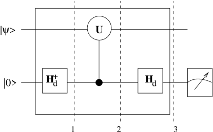
Figure 5: Diagram depicting the circuit for ‘outsourcing’ measurement on a $d$ dimensional system (upper wire) to an ancilla (lower wire). The circle-link represents the generalized controlled-$U$ operation. The dashed lines depict the three stages of the outsourcing operation preceding measurement of the ancilla.

It follows from the above that if $|j;k\rangle$ is an eigenstate of $U$, then the outsourced measurement of $W$ on $|j;k\rangle$ will be non-destructive but return the value $j$. This gives us the following corollary.

Corollary 1

If $U_{1}$ and $U_{2}$ are commuting unitary operators, then the corresponding outsourced observables $W_{1}$ and $W_{2}$ can be simultaneously measured.

If the operator $U$ is a product of operations on subsystems, then the control-operation can be done pair-wise on each subsystem and a common ancilla, before the ancilla is finally measured. This is proved in Theorem 2.

Theorem 2

The outsourced measurement of observable $W$ compatible with unitary operator $U=\bigotimes_{m}U_{m}$, where $m$ ($=1,2,\cdots,n$) labels the subsystems, can be performed by separate control-operations on the individual subsystems $j$ from the same ancilla. The control-operations may be performed in any order.

Proof. Note that ${\cal C}_{U}=\sum_{j}|j\rangle\langle j|\bigotimes_{m}(U_{m})^{j}=\left(\sum_{j}|j\rangle\langle j|\otimes(U_{1})^{j}\otimes\mathbb{I}^{\otimes(m-1)}\right)\left(\sum_{j^{\prime}}|j^{\prime}\rangle\langle j^{\prime}|\otimes\mathbb{I}\otimes(U_{2})^{j^{\prime}}\otimes\mathbb{I}^{\otimes(m-2)}\right)\cdots$ $\left(\sum_{j^{\prime\prime}}|j^{\prime\prime}\rangle\langle j^{\prime}|\otimes\mathbb{I}^{\otimes(m-1)}(U_{2})^{j^{\prime\prime}}\right)$. Therefore ${\cal C}_{U}={\cal C}_{U_{1}}\times{\cal C}_{U_{2}}\times\cdots{\cal C}_{U_{m}}$, where ${\cal C}_{U_{k}}\equiv\sum|j\rangle\langle j|\otimes(U_{k})^{j}$. Since the ${\cal C}_{U_{j}}$’s commute with each other, they may be performed in any order. $\Box$

However, note that though the control operations are separable, there is a quantum communication of the ancilla along the chain formed by the players. The measurement of $M_{1}$ in the preceding Section can be seen as a special case of Theorems 1 and 2. To see this, we set $U\equiv X^{\otimes n}$, where each $U_{i}=X_{d}$. Since $X^{\otimes n}|\Psi_{pq_{1},\cdots,q_{n-1}}\rangle=e^{2\pi\iota p/d}|\Psi_{pq_{1},\cdots,q_{n-1}}\rangle$, by Theorem 1, the observable $M_{1}\equiv\sum_{p,q_{1},\cdots}f(p)|\Psi_{pq_{1},\cdots,q_{n-1}}\rangle\langle\Psi_{pq_{1},\cdots,q_{n-1}}|$ can be outsourced using the control operation ${\cal C}_{U}\equiv\sum|j\rangle\langle j|\otimes U^{j}$. In view of Eq. (5b), this has the effect: ${\cal C}_{U}:|j\rangle|j_{1}\rangle\cdots|j_{n}\rangle\longmapsto|j\rangle|j_{1}+j\rangle\cdots|j_{n}+j\rangle$. It then follows from Theorem 2 that ${\cal C}_{U}$ can be broken into $n$ applications of ${\cal C}_{X}$ operations on an ancilla-qudit pair, for each qudit of the system and a fixed ancilla, where ${\cal C}_{X}$ is precisely the operation defined in Eq. (8). In a distributed computing scenario, this ancilla must be sequentially interacted with each system qudit. This clarifies our use of the Eq. (8) as the generalization of the CNOT gate. We also obtain the general Bell state discrimination circuit described in Eq. (11a) as a special case of Theorems 1 and 2.

In general, given any set of orthonormal states that form a complete basis to an observable $W$, Theorem 1 allows us to ‘outsource’ their measurement to an ancilla. To do so, we first construct a unitary operator $U$ with respect to which these states are ‘dark’, i.e., of which these states are eigenstates, and using this to construct a control-$U$ operation ${\cal C}_{U}$. If $U$ is separable, as is the case in our problem, then Theorem 2 allows ${\cal C}_{U}$ to be broken up into a sequence of pair-wise control gates.

Consider measurement of the relative parity observable $Z_{d}(i-1)\otimes Z_{d}^{{\dagger}}(i)$. Following Theorems 1 and 2, the measurement here can be outsourced using control-$Z_{d}^{{\dagger}}$ (${\cal C}_{Z_{d}^{{\dagger}}}$) and control-$Z_{d}$ (${\cal C}_{Z_{d}}$) operations from the ancilla sequentially to the two qudits. According to Eq. (5a), these require controlled-phase operations. However, by means of applying Hadamards, it is possible to turn them into ${\cal C}_{X}$ operations. To see this, we note that for any integer $j$,

$$(Z^{{\dagger}}\otimes Z_{d})^{j} = (Z^{{\dagger}}_{d})^{j}\otimes(Z_{d})^{j}$$ (15)

$$= (H_{d}X^{{\dagger}}_{d}H^{{\dagger}}_{d})^{j}\otimes(H_{d}X_{d}H^{{\dagger}}_{d})^{j}$$

$$= (H_{d}(X^{{\dagger}}_{d})^{j}H^{{\dagger}}_{d})\otimes(H_{d}(X_{d})^{j}H^{{\dagger}}_{d})$$

$$= (H_{d}\otimes H_{d})\times(X^{{\dagger}}_{d}\otimes X_{d})^{j}\times(H^{{\dagger}}_{d}\otimes H_{d}^{{\dagger}}).$$

This means that the outsourcing of measurement of $Z_{d}^{{\dagger}}\otimes Z_{d}$ is equivalent to the circuit in Fig. 6(a), where only ${\cal C}_{X}$ and ${\cal C}_{X}^{{\dagger}}$ are used.

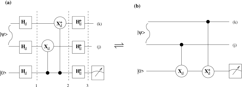
Figure 6: The two circuits are equivalent to outsourcing measurement of $Z_{d}\otimes Z_{d}^{{\dagger}}$ on any two wires of an $n$-qudit state. The Hadamards serve the role of reversing the direction of control in the control gates.

The last result we require says that, by dropping the Hadamards in Fig. 6(a), we can reverse the control direction. This is shown in Theorem 3. Two advantages of such a step is that for each outsourced measurement of $Z^{{\dagger}}_{d}\otimes Z_{d}$, the number of Hadamards is reduced by a factor of six and furthermore instances of only one nonlinear gate (namely, ${\cal C}_{X_{d}}$ or ${\cal C}_{X_{d}^{{\dagger}}}$) need to be used.

Theorem 3

The two measurement circuits depicted in Fig. 6 are equivalent.

Proof. Let the incoming state of the two system wires be the pure state $|\Psi\rangle=\sum_{jk}\alpha_{jk}|j\rangle|k\rangle$ (we ignore the fact that the summation can run on a single index on account of Schmidt decomposability). At stage 1, the state of the ancilla-system complex is: $(1/\sqrt{d})\left(\sum_{l}|l\rangle\right)\left(\sum_{j,k,j^{\prime},k^{\prime}}\alpha_{jk}\exp[(2\pi\iota/d)(-jj^{\prime}+kk^{\prime})]|j^{\prime}\rangle|k^{\prime}\rangle\right)$. By the action of the two control-gates, the state in stage 2 is $(1/\sqrt{d})\left(\sum_{l,j,k,j^{\prime},k^{\prime}}\alpha_{jk}\exp[(2\pi\iota/d)(-jj^{\prime}+kk^{\prime})]|l\rangle|j^{\prime}-l\rangle|k^{\prime}-l\rangle\right)$. In stage 3, by the action of the three Hadamards, the state $|\Psi^{\prime}\rangle$ of the complex is

$$|\Psi^{\prime}\rangle = (1/\sqrt{d})\left(\sum_{l,j,k,j^{\prime},k^{\prime},j^{\prime\prime},k^{\prime\prime}}\alpha_{jk}\exp\left[(2\pi\iota/d)(-jj^{\prime}+kk^{\prime}-ll^{\prime}+j^{\prime\prime}[j^{\prime}-l]-k^{\prime\prime}[k^{\prime}-k])\right]|l^{\prime}\rangle|j^{\prime\prime}\rangle|k^{\prime\prime}\rangle\right)$$ (16)

$$= (1/\sqrt{d})\left(\sum_{l,j,k,j^{\prime},k^{\prime},j^{\prime\prime},k^{\prime\prime}}\alpha_{jk}\exp[(2\pi\iota/d)(l(-l^{\prime}-j^{\prime\prime}+k^{\prime})+j^{\prime}[j^{\prime\prime}-j]+k^{\prime}[k-k^{\prime\prime}])]|l^{\prime}\rangle|j^{\prime\prime}\rangle|k^{\prime\prime}\rangle\right)$$

$$= (1/\sqrt{d})\left(\sum_{l,l^{\prime},j,k}\exp[(2\pi\iota/d)(l(-l^{\prime}-j+k)]|l^{\prime}\rangle|j\rangle|k\rangle\right)$$

$$= \sum_{j,k}\alpha_{jk}|k-j\rangle|j\rangle|k\rangle,$$

which is the situation described by the circuit in Fig. 6(b). In general, the two wires, being part of a larger system, are in a mixed state. Since a mixed state can be regarded as an ensemble of pure states, Eq. (16) implies the equivalence of the circuits in the Fig. 6(a) and 6(b) even for mixed states. $\Box$

From Theorems 1, 2 and 3, it follows that the circuitry described by Eq. (11b), or equivalently, depicted in the second bounded box of Fig. 3, indeed outsources measurement of $Z_{d}\otimes Z^{{\dagger}}_{d}$. More generally, Theorem 3 can be used to reverse the direction of control in the outsourcing of two-qudit observables, by replacing $U$ with $H_{d}UH_{d}^{{\dagger}}$ as the unitary operator on which the control gate is based.

V Some applications

Such non-destructive state discrimination can be useful in distributed quantum computing, especially when there are restrictions coming from the topology of the quantum communication network. Unlike their classical counterparts, quantum channels are expected to be expensive and not amenable to change to suit a problem at hand. Rather, it is worthwhile to use protocols that minimize quantum communication complexity, that is, the quantity of quantum information that must be communicated between different parties to perform a computation or process some information, in a given network.

A simple way to perform Bell state discrimination is for all other members to communicate their qudits to single station, whose member (called, say Alice) performs a joint measurement on all $n$ qubits or qudits to determine the state. She then re-creates the measured state and transmits them for further use. Actually, in the present situation, instead of a joint measurement on all qubits, Alice can apply a string of $n-1$ ${\cal C}_{X}^{{\dagger}}$ operations on each consecutive pair of qudits in the Bell state $|\Psi_{pq_{1}q_{2}\cdots q_{n-1}}\rangle$ and $H^{{\dagger}}_{d}$ finally on the first qudit. It is easily seen that each application of ${\cal C}_{X}^{{\dagger}}$ will disentangle the controlled qudit from the rest. For the Bell states, this procedure effects the transformation:

$$|\Psi_{pq_{1}q_{2}\cdots q_{n-1}}\rangle~{}\longmapsto~{}|p\rangle|q_{2}-q_{1}\rangle\cdots|q_{n-1}-q_{n-2}\rangle.$$ (17)

Subsequent measurement of each qudit in the computational basis completely characterizes the Bell state. The Bell state thus being discriminated, the above procedure can be reversed to re-create the state $|\Psi_{pq_{1}q_{2}\cdots q_{n-1}}\rangle$ and transmit it back to the remaining players.

Irrespective of network topology, such a disentangle-and-reentangle strategy requires in all $2(n-1)$ two-qudit gates to be implemented. In our method, the number of two-qudit gates is the sum of $n$ two-qudit gates for determining phase parameter $p$ and $2(n-1)$ for determining the (relative) parities, giving $3n-2$ two-qudit gates. From this viewpoint of consumption of nonlinear resources, our method does not offer any advantage. However, this turns out not to be the case from the viewpoint of quantum communication complexity.

Suppose a quantum communication network with a star topology and $n$ members is given, as for example in Fig. 4(a). For all members to transmit their qudits to Alice (at $A$), and for her to transmit them back would require $2(n-1)$ qudits to be communicated, where the factor 2 comes from the two-way requirement. In our protocol, one way quantum communication suffices. For measuring the ‘phase observable’ $M_{1}$, the number of qudits communicated is seen to be $2(n-1)$, since the ancilla must pass through the hub to reach each member on a single-edge vertex; and if measured edgewise, the communication complexity for relative parity measurement is $n$ qudits. In all, this requires $3n-2$ qudits to be communicated, which is larger than that required for a plain disentangle-reentangle method.

However consider a linear configuration of the communication network, as in Fig. 4(b), where members are linked up in a single series. In the disentangle-reentangle method, if Alice is located at one end, the communication complexity is seen to be $n(n-1)$ qudits; it is $(n^{2}-1)/2$ if she is in the middle. In either case, it is of order $O(n^{2})$. In contrast, our non-destructive method can be implemented using $n-1$ qudits communicated both for phase and relative parity measurement, requiring in all only $2(n-1)$ qudits to be communicated, so that the required communication is only of order $O(n)$. Thus our method gives a quadratic saving in quantum communication complexity.

A further advantage, that may be of some importance in certain situations, is that our method divides the required resources in terms of applying nonlinear gates and of measurements equally among the various members. In a real life situation, this may facilitate the distribution of quantum information processing resources among the various members.

Appendix A Closure of generalized Bell states under Hadamards

The action of $H\otimes H^{{\dagger}}$ on $|\Psi_{pq}\rangle$ on the states in Eq. (9) produces the effect of effectively interchanging the indices $pq$ of $|\Psi_{pq}\rangle$:

$$(H\otimes H^{{\dagger}})|\Psi_{pq}\rangle = \frac{1}{\sqrt{d}}\sum_{j,k,l}e^{(2\pi\iota/d)(j[p+k-l]-ql)}|k\rangle|l\rangle$$ (18)

$$= \frac{1}{\sqrt{d}}\sum_{j,l}e^{(2\pi\iota/d)(-ql)}|l-p\rangle|l\rangle$$

$$= \frac{1}{\sqrt{d}}\sum_{j}e^{(2\pi\iota/d)([d-q]l)}|j\rangle|j+p\rangle,$$

$$= |\Psi_{q^{\prime}p}\rangle,$$

where $q^{\prime}=(d-q)~{}\mod~{}d$ and the second step follows from noting that the only non-zero contributions come for the case $p+k-l=0$, and an overall phase factor has been dropped in the third step. Similarly, one finds $(H\otimes H^{{\dagger}})|\Psi_{pq}\rangle=|\Psi_{qp^{\prime}}\rangle$, where $p^{\prime}=d-p$ mod $d$.