Strategies for Real-Time Position Control of a Single Atom in Cavity QED

Abstract

Recent realizations of single-atom trapping and tracking in cavity QED open the door for feedback schemes which actively stabilize the motion of a single atom in real time. We present feedback algorithms for cooling the radial component of motion for a single atom trapped by strong coupling to single-photon fields in an optical cavity. Performance of various algorithms is studied through simulations of single-atom trajectories, with full dynamical and measurement noise included. Closed loop feedback algorithms compare favorably to open-loop “switching” analogs, demonstrating the importance of applying actual position information in real time. The high optical information rate in current experiments enables real-time tracking that approaches the standard quantum limit for broadband position measurements, suggesting that realistic active feedback schemes may reach a regime where measurement backaction appreciably alters the motional dynamics.

I Introduction

Recent experiments acm ; pinkse ; fort ; mckeever ; mcknature have demonstrated the ability to trap acm ; fort ; mckeever ; mcknature ; rempe-nature and localize pinkse a single atom in a high-finesse optical cavity by way of optical forces. Moreover, by detecting the light transmitted by the cavity, the atom’s motion within the cavity mode can be monitored in real time with high signal to noise throughout its trapped lifetime acdpra .These achievements in trapping and localization open up exciting possibilities for quantum logic and quantum state preparation in the context of cavity QEDcirac98 ; pcz ; cirac97 ; vanenk98 ; briegelrep ; briegelnet . Beyond the realization of trapping, the high signal-to-noise for continuous, real-time position measurement is itself one of the most notable features of these strongly coupled cavity QED systems. Such detailed real-time position information immediately suggests the idea of active feedback to dynamically cool the motion of a single trapped atom. By investigating this system and the feedback schemes available in it, basic questions of quantum state estimation and optimal control can be explored for continuous measurement of a dynamical variable – in this case the position of a single atom.

Crucial to the realization of trapping and sensing in cavity QED is strong coupling, a condition in which the coherent coupling between atom and cavity field dominates dissipative rates in the system. For a two-state atom optimally coupled to the cavity mode, the dipole-field coupling is given by the Jaynes-Cummings interaction Hamiltonian jc

$$H_{int}=\hbar g(\sigma_{+}a+\sigma_{-}a^{{\dagger}}),$$ (1)

where $\sigma_{\pm}$ are dipole raising and lowering operators, $(a,a^{{\dagger}})$ are field annihilation and creation operators for the cavity mode, and $g$ is one half of the single-photon Rabi frequency. This interaction gives rise to the well-known Jaynes-Cummings ladder of eigenstates for the coupled atom-cavity system, and correspondingly to the vacuum Rabi splitting for the system’s resonant frequencies eberly . Dissipation, on the other hand, is characterized by the cavity decay rate $\kappa$ and the atomic spontaneous emission rate $\gamma$. Strong coupling occurs for $g\gg(\kappa,\gamma)$. We can define a further condition of strong coupling for the external atomic degrees of freedom; this occurs when the coherent coupling also dominates the atomic kinetic energy, as first achieved in Ref. HoodPRL .

Under these conditions, interaction with a single-photon cavity field exerts a strong mechanical effect on a single atom, allowing trapping of the atom when the system is driven to strong-field seeking states in the Jaynes-Cummings ladder. Furthermore, strong coupling assures that the intracavity light field and thus the cavity output field (transmitted light) are influenced by an atom; thus, as an atom moves between more and less strongly coupled positions within the cavity, the transmitted light provides a real-time measurement of atomic position. This sensing enables the one-time triggering employed in Refs. acm ; mckeever ; pinkse ; fort to switch on a trapping potential when an atom is present near the center of the cavity. The ongoing stream of position information should, however, be useful for continued active feedback based on the atomic position. Rather than simply triggering a potential to turn on, it should be possible to modulate the potential depth to dynamically cool the atomic motion, in a method analogous to the principles of stochastic cooling but for a single atom. Initial steps in this direction are represented in the work of Ref. rempefb . Quantum feedback for other atomic state variables is also an active area of research, including the recent experimental demonstration of quantum feedback to control the ensemble spin of a collection of cold atoms hmspinexpt .

In this paper, we address the question of how to implement atomic position feedback in experimentally realistic situations, where several constraints apply: (1) the system is inherently nonlinear and largely nonanalytic, with relationships between many quantities of interest determined by steady-state solutions to the master equation for the atom-cavity system, (2) dynamical noise is significant and changes in tandem with the driving field and trapping potential, and (3) measurement noise, arising largely from the fundamental quantum noise (shot noise) of detection, imposes necessary delays in the estimation of dynamical variables and the implementation of feedback. Broadband measurement near the standard quantum limit (see Ref. sql ) has been demonstrated in this system through measurement of cavity transmission amplitude acm and by simultaneous measurement of transmitted amplitude and phase fullmeas . Use of these measurements in feedback control of some aspect of the atomic motion should bring us closer to regimes where measurement backaction has a significant effect, so that different detection methods may exhibit different control limits based on these effects as well as on more conventional signal-to-noise considerations andreis ; gambetta .

In Section II we review the experimental system on which our work is based. The feedback strategy we consider is presented and motivated in Section III. Section IV presents feedback results; these are considered both in the realistic experimental context and in several idealized systems in order to illustrate the algorithm’s effect on the individual components of atomic motion. In Section V we again take up the topic of experimentally measurable feedback results, and in Section VI we discuss limits and possible extensions of the algorithms discussed in the paper.

II Experimental Status and Sensitivity for Atomic Position Measurement

In our feedback calculations, we have considered the situation of Ref. acm , where a single atom is trapped via its interaction with a near-resonant cavity light field at the level of a single photon. In that experiment, the small saturation photon number and critical atom number hjkscripta – the smallest in experiments to date – facilitated not only the trapping mechanism but, more importantly for these considerations, the high signal-to-noise observation of atomic motion within the cavity field.

Figure 1 shows a schematic diagram of the experimental procedure, in which Cesium atoms (atomic resonance frequency $\omega_{a}$) are collected in a magneto-optical trap (MOT) directly above the cavity mirrors, cooled to temperatures of $\sim 10\mu$K, and dropped through the cavity. The geometry of the mirror substrates cuts off most of the atomic flux so that one atom at a time transits the cavity mode of length $l$ and Gaussian waist $w_{0}$. The cavity resonance $\omega_{c}$ is tuned near but slightly below the atomic resonance frequency so that $\omega_{c}-\omega_{a}<0$. The cavity is continuously driven by a probe laser at frequency $\omega_{p}$, and the transmission of this beam through the cavity is monitored via balanced heterodyne detection. For a probe red-detuned from both atom and cavity ($\omega_{p}$ near the lower vacuum Rabi sidebandeberly ), transmission is low for the empty cavity and is highest when an atom is in the regions of strongest coupling. Thus the monitored photocurrent carries real-time information about the atomic position, with high signal-to-noise even for probe strengths corresponding to $<1$ intracavity photons. Saturation of the atom-cavity responseHoodPRL sets in for larger field strength, so that the most sensitive tracking is realized at $\sim 1$ intracavity photon.

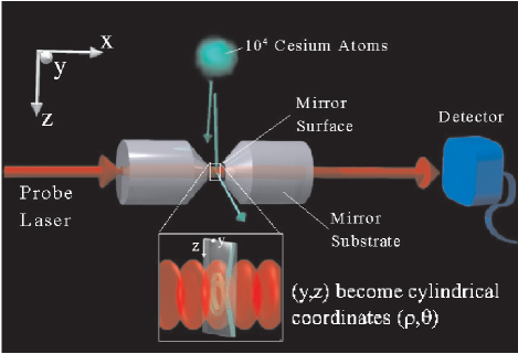
Figure 1: Cesium atoms are dropped from a MOT and a small fraction of these fall one by one through the mode of an optical cavity. The cavity mode is a cylindrically symmetric Gaussian in the transverse $(\rho,\theta)$ plane and has a standing-wave structure in the axial (x) direction. Transmission of a probe beam through the cavity is monitored to sense an atom’s motion through the cavity mode; a detected rise in transmission triggers a switch to higher probe intensity, significantly populating strong-field-seeking states of the atom-cavity system and thus trapping the atom. The figure shows one falling atom which misses the cavity mode altogether and a second atom which enters the cavity, is trapped in the mode, and eventually escapes.

The atom-cavity evolution in this system is described by a master equation (see, e.g., api ; masterequation ; tan1999a ) for the joint atom-cavity density operator $\rho$. We consider a driving (and probing) field $\epsilon$ of frequency $\omega_{p}$, a cavity resonant at $\omega_{c}=\omega_{p}+\Delta_{cp}$, and an atomic resonance frequency $\omega_{a}=\omega_{p}+\Delta_{ap}$. In the electric dipole and rotating-wave approximations, and in the interaction picture with respect to the probe frequency, the master equation can be written

$$\dot{\hat{\rho}}=-\frac{i}{\hbar}[\hat{H}_{0},\hat{\rho}]+\gamma(2\hat{\sigma}\hat{\rho}\hat{\sigma}^{{\dagger}}-\hat{\sigma}^{{\dagger}}\hat{\sigma}\hat{\rho}-\hat{\rho}\hat{\sigma}^{{\dagger}}\hat{\sigma})$$

$$+\kappa(2\hat{a}\hat{\rho}\hat{a}^{{\dagger}}-\hat{a}^{{\dagger}}\hat{a}\hat{\rho}-\hat{\rho}\hat{a}^{{\dagger}}\hat{a}),$$ (2)

$$\hat{H}_{0}=\hbar\Delta_{cp}\hat{a}^{{\dagger}}\hat{a}+\hbar\Delta_{ap}\hat{\sigma}^{{\dagger}}\hat{\sigma}+\hbar g(\vec{r})[\hat{a}\hat{\sigma}^{{\dagger}}+\hat{a}^{{\dagger}}\hat{\sigma}]$$

$$+\hbar\epsilon(\hat{a}+\hat{a}^{{\dagger}}).$$ (3)

Here $g(\vec{r})$ is the coupling strength which takes into account the atomic position $\vec{r}$ within the cavity mode. For a Fabry-Perot cavity supporting a standing wave mode with Gaussian transverse profile, $g(\vec{r})=g_{0}cos(2\pi x/\lambda)exp[-(y^{2}+z^{2})/w_{0}^{2}]$. The cylindrical symmetry of the field suggests the use of cylindrical coordinates $(\rho,\theta,x)$, where $\rho=\sqrt{y^{2}+z^{2}}$ and $\theta=tan^{-1}(-z/y)$ (see Figure 1). Thus we write $g(\vec{r})=g_{0}cos(2\pi x/\lambda)exp[-\rho^{2}/w_{0}^{2}]$. In the fully quantum treatment, the atomic position $\vec{r}$ is itself an operator; in experiments to date a quasi-classical treatment suffices, so the atom may be considered a wavepacket with $\vec{r}$ a classical center-of-mass position variable. Similar feedback schemes for an atom-cavity system have also been explored theoretically in the case of an atom which has already been cooled radially and must now be treated in a fully quantized manner for cooling of the remaining axial motionsteckfb .

Following the experimental situation of Ref.acm , we consider an atom-cavity system in which $(g_{0},\kappa,\gamma)/2\pi=(110,14.2,2.6)$ MHz. The simulation results below refer to varying cavity field strength but with detunings fixed at $(\omega_{c}-\omega_{a})/2\pi=-47$ MHz, $(\omega_{p}-\omega_{a})/2\pi=-125$ MHz.

Figure 2(a) shows the first few levels of the Jaynes-Cummings ladder of energy eigenvalues, obtained by diagonalizing the interaction Hamiltonian of Eq. 3. The smooth evolution from uncoupled to fully coupled eigenstates reflects the dependence of coupling $g(\vec{r})$ on the atomic position $\vec{r}$, and specifically on the atom’s distance $\rho$ from the cavity axis. In the presence of dissipation and driving, the distribution of populations across the first few levels of this ladder is determined by numerical steady-state solution of the master equation at each position. Figure 2(b) shows the effective potential for the atom-cavity properties considered in this work, with driving level in this example fixed at $n_{hi}$=0.3 photons in the empty cavity. The atom-trapping scheme of acm is based on tracking the atomic position and altering the driving field strength to place the system in the attractive potential of Figure 2(b) when the atom is close to the cavity axis ($\rho\approx 0$).

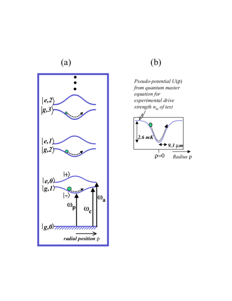
Figure 2: (a)First few levels of the ladder of energy eigenstates for the atom-cavity system. Uncoupled and maximally coupled eigenvalues are illustrated, along with their smooth dependence on the atomic position (and hence the atom-cavity coupling). Strength of driving light determines the system’s population distribution across the first few levels of the ladder, setting the shape and depth of the effective potential. (b) Effective potential for the atom, cavity, and probe detuning parameters of the simulations, and drive strength $n_{hi}$ corresponding to 0.3 photons in the empty cavity on resonance.

Figure 3(a) shows a sample experimental trace of transmission vs. time for a single atom trapped as in Ref. acm . Immediately notable in the transmission record are the large, regular oscillations in the heterodyne current, which can be associated with an atom repeatedly approaching and receding from the regions of strongest atom-cavity coupling. The cavity mode structure produces a trapping potential with width $\sim\lambda/2=426$nm in the axial direction and $\sim w_{0}=14\mu$m in the radial direction, giving axial oscillations at $\sim 1-2$MHz while radial oscillations occur on the much slower timescale of $\sim 10-20$kHz. By using a detection bandwidth of 100kHz, we obtain a transmission record that averages over the effects of axial motion.

(a)

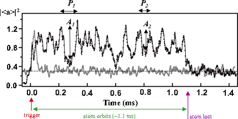
(b)

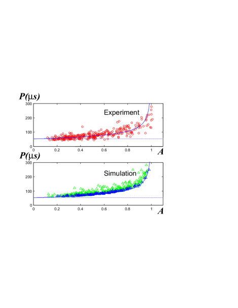
Figure 3: (a) Cavity transmission record for an atom trapped with 0.3 photons in the empty cavity. Motion of the trapped atom within the cavity mode can be tracked via the oscillations in cavity transmission. Each oscillation has amplitude A and period P as indicated on the trace. (b) Oscillation period P vs. amplitude A of transmission oscillations as in (a). The solid curve is calculated for motion in the known anharmonic potential of Figure 2(b), with no free parameters in the fit.

A series of quantitative comparisons demonstrates that the remaining transmission signal faithfully reflects radial motion with very little contamination from the axial averagingacdpra . Simulations indicate that, for the parameter regime employed in Ref.acm , a trapped atom is typically confined within $\sim 50nm$ of a single standing-wave antinode until it heats very quickly and escapes the trap altogether. Events involving large-amplitude oscillations or ‘skipping’ across wells and retrapping in another antinode are very rare occurrences in this regime; since axial motion typically has such small amplitudes, we expect the average over it to have a negligible effect on measured cavity transmission. Comparison of observed maximum transmission levels with the expected theoretical maximum confirms this notion, giving an estimate of $\lesssim 75nm$ for typical axial excursions.

As further confirmation that transmission accurately reflects radial motion, we consider the observed period of transmission oscillations as a function of their amplitude. From our knowledge of the anharmonic (approximately Gaussian) trapping potential in the radial direction, it is straightforward to calculate the expected relationship between amplitude and period for these oscillations. As evident from Figure 3(b), actual data closely follow the theoretical curve, indicating that the transmission record can indeed be interpreted as a record of radial motion ($T(t)\rightarrow\rho(t)$). Though the atom-cavity coupling is cylindrically symmetric and thus provides no explicit information about $\theta(t)$, knowledge of $\rho(t)$ and the trapping potential allow us to reconstruct an estimate of an atom’s angular momentum $L(t)$ and thus of a two-dimensional trajectory in the $(\rho,\theta)$ plane. Such a method can be applied with success in a parameter regime where the atomic motion is largely conservative and the angular momentum varies slowly on the timescale of a single radial orbitacm ; acdpra .

Three basic ambiguities will be clear from this algorithm for trajectory reconstruction: 1) the sign of the angular momentum is unknown, so the trajectory has arbitrary handedness. 2) the initial angle $\theta_{0}$ is arbitrary, so the resulting trajectory can be rotated freely as a unit. 3) The trajectory is constructed in two dimensions, with the axial motion confined within a single antinode, but no information is available about which antinode the atom occupies during the trajectory. These ambiguities, while noted here for clarity, arise in aspects of the motion not used in the feedback scheme treated below.

Two-dimensional trajectory reconstructions dramatically illustrate the cavity-enhanced sensing power for atomic motion. However, the initial goal of our feedback algorithms will be to control $\rho(t)$; for this purpose it is sensible to ignore $\theta(t)$ and apply all available signal to noise to the task of estimating $\rho(t)$ and $\dot{\rho}(t)$ in real time. The goal of such a program is then to use this information to drive $\rho(t)$ to a constant value, or in other words to circularize an orbit in the $(\rho,\theta)$ plane while not necessarily driving it to the cavity axis ($\rho=0$). The latter task, which requires an explicit method of breaking cylindrical symmetry for position sensing and for the effective potential, can be considered as a later extension.

III The Atom and Cavity as a Control System: Basic Feedback Strategy

As a guide in the identification of plausible feedback strategies and their limitations, it is useful to restate the problem somewhat in the language of control systems. To this end, we begin by setting aside the issue of axial motion and treating the atom as a particle in a cylindrically symmetric, approximately Gaussian two-dimensional potential whose depth is controlled by the input light intensity:

$$U\approx-U_{0}e^{-\rho^{2}/w^{2}}.$$ (4)

Note that the potential waist $w$ is not simply equated with the previously introduced cavity field waist $w_{0}$ or with the mode intensity waist $w_{0}/\sqrt{2}$, but rather is set by the self-consistent interaction of atom and light field in the strong coupling regime. Whereas the cavity mode profile is exactly Gaussian, $U$ is only approximately Gaussian and has an exact form that is nonanalytical as determined by steady-state solutions to the master equation for an atom at each value of $\rho$. The potential depth $U_{0}$ depends on the intensity of the optical field used to drive the cavity mode. The potential waist $w$ is in fact a (slowly varying) function of the drive strength as well acdpra .

The trapped atom is also subject to friction and to dynamical noise (momentum diffusion), both arising from decays and re-excitations of the system on timescales faster than the motion. In the regime of Ref. acm , the contribution of friction is small compared to the momentum diffusion terms in the equation of motion.

Because the two-dimensional potential is symmetric, the atom’s angular momentum $L$ is constant, or rather, varies only due to dynamical noise. We can thus write a one-dimensional effective potential in the $\rho$ dimension,

$$V_{eff}=-U_{0}e^{-\rho^{2}/w^{2}}+L^{2}/2m\rho^{2}$$ (5)

and thus an equation of motion (for an atom of mass $m$)

$$\ddot{\rho}=-\frac{2\rho U_{0}}{mw^{2}}e^{-\rho^{2}/w^{2}}+\frac{L^{2}}{m^{2}\rho^{3}}$$ (6)

which we notationally simplify to the form

$$\ddot{\tilde{\rho}}=-\tilde{\rho}Ee^{-\tilde{\rho}^{2}}+\frac{\tilde{L}}{\tilde{\rho}^{3}}$$ (7)

where $\tilde{\rho}$ is dimensionless ($\tilde{\rho}=\rho/w$), $E=2U_{0}/mw^{2}$ is the input we control by varying the driving field strength, and $\tilde{L}=L^{2}/m^{2}w^{4}$ is constant except for the influence of friction and dynamical noise.

The measurement of light transmitted through the cavity, $T(t)$, is equivalent to a (noisy) measurement of $\rho(t)$. The noise of this measurement is largely fundamental quantum noise (shot noise) of detection. The mapping between $T$ and $\rho$, derived again from steady-state solutions of the master equation for the coupled atom-cavity system, is not linear and furthermore depends on the value of the driving strength $E$. The initial objective is to circularize the two-dimensional orbit – in other words, to make $\rho$ constant or to hold $\dot{\rho}=0$ by varying the control input $E$.

The simplified system can be described by a block diagram as shown in Figure 4. The system exhibits myriad nonlinearities; for example, ($T\rightarrow\rho$) is nonlinear and depends on $E$, the dynamical noise depends on $E$, and the equation of motion for $\rho$ is itself nonlinear. Nonetheless, while this statement of the problem does not suggest provably optimal feedback strategies, it does motivate some conceptually simple algorithms based on switching between discrete values of driving strength $E$. Switching strategies of this sort are often invoked for the sake of robustness, a major consideration in this scenario; robustness to dynamical and measurement noise is certainly important, but perhaps even more relevant is robustness to small uncertainties in system parameters (e.g., driving strengths or detunings). Switching or “bang-bang” type algorithms controltheory have the additional virtue of admitting easy implementation in simulations and in experimental design.

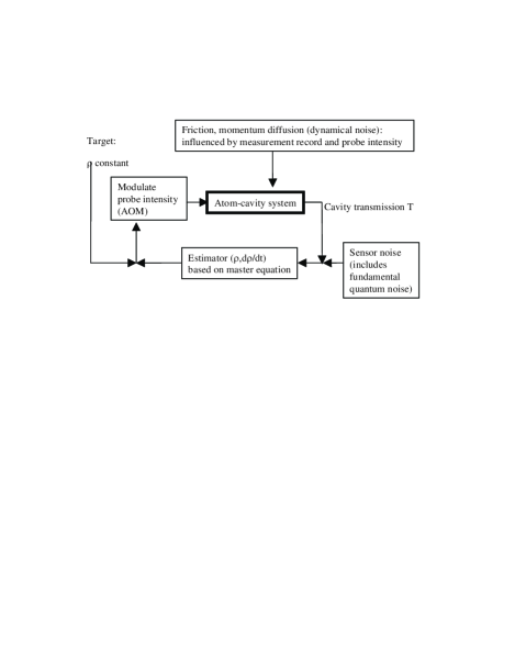
Figure 4: Block diagram for the atomic position feedback loop, illustrating sources of noise and system nonlinearities.

The feedback algorithms we investigate in this paper all share the same basic strategy of switching the driving field intensity between two discrete levels. This corresponds to switching between two potential depths (and, incidentally, two different sets of friction and momentum diffusion coefficients as well). The simple objective is to time this switching relative to the atomic motion so that an atom sees a steep potential when climbing out of the trap ($\dot{\rho}>0$) and a shallow potential when falling back towards the trap center ($\dot{\rho}<0$), as illustrated in Figure 5. The feedback algorithm, then, is based on switching the potential at turning points of $\rho$, i.e., each time $\dot{\rho}$ crosses zero. Implemented effectively, this approach promises significant dynamical cooling of the radial motion ($\rho\rightarrow constant$ or $\dot{\rho}\rightarrow 0$) in just a few oscillations.

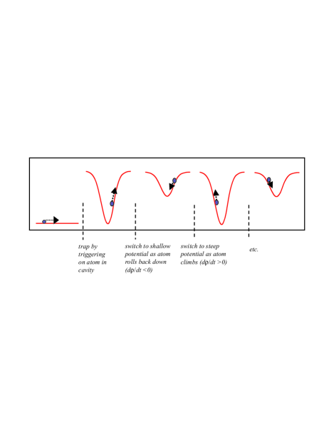
Figure 5: General feedback strategy for atomic radial coordinate.

The initial detection and trapping of an atom are accomplished as in Ref. acm ; acdpra ; a weak probe at driving level exlo is used to detect the atom’s arrival in the cavity with minimal effect on the motion, and an increase in transmission of this beam triggers a switch to driving level hi to populate strong-field-seeking states and trap the atom. Feedback is then implemented by switching the trapping potential between the hi level and an intermediate lo setting, with switching times based on real-time information about the motion of the single atom.

The simplest algorithm would be to switch back and forth between hi and lo potentials at the turning points of $\rho(t)$, which are the zero-crossings of $\dot{\rho}(t)$. That is, trap initially in hi, switch to lo when $\dot{\rho}$ crosses zero from above (i.e., when $\rho$ begins to decrease), switch back to hi when $\dot{\rho}$ crosses zero from below ($\rho$ reaching its minimum and increasing), and so on until the atom escapes. However, this strategy calls for a theoretically infinite sequence of switching events, while it is desirable to instead achieve a steady state in some long-time limit. The presence of dynamical noise implies that the exact steady state of $\dot{\rho}\rightarrow 0$ is in any case unreachable, so we replace it with a goal of confining $\dot{\rho}$ to some range $[-lim,+lim]$. Thus the feedback strategy is modified to include slight hysteresis: lo$\rightarrow$hi when $\dot{\rho}\rightarrow+lim$ from below, hi$\rightarrow$lo when $\dot{\rho}\rightarrow-lim$ from above. With this modification, switching stops once $\dot{\rho}$ is confined within the acceptable range. Furthermore, we prefer a steady state with hi potential for reasons of the deeper confinement; to bias the system towards this final state, we use asymmetric hysteresis limits: lo$\rightarrow$hi when $\dot{\rho}\rightarrow+lim$ from below, hi$\rightarrow$lo when $\dot{\rho}\rightarrow-(lim+\delta)$ from above.

IV Simulations of Feedback Algorithms in Operation

For our simulations, we first choose driving strengths $n_{exlo}=0.05$ photons in the empty cavity, $n_{hi}=0.3$ photons in the empty cavity, and $n_{lo}=0.15$ empty-cavity photons. These driving strengths are high enough so that an atom of typical kinetic energy can be trapped by both lo and hi drives, yet low enough to ensure the increase in momentum diffusion between lo and hi does not outstrip the increase in potential depth.

Our simulations of the atom-cavity dynamics are based on the treatment described in detail in Ref. acdpra ; acd ; the treatment is fully quantized for the atomic internal state and the cavity light field, but considers the atomic center-of-mass motion quasiclassically. This approximation is suitable for the current experimental situation, with more manifestly quantized motion to be accessed by better cooling and/or detection of the atom’s axial motion. The non-conservative terms in the system, in the form of friction and momentum diffusion, are included in the simulation; the resulting “heterodyne transmission” trace is a perfect record of $|\langle a\rangle|^{2}$, on which measurement bandwidths and shot noise must be imposed separately. Shot noise is modelled as Gaussian white noise with an amplitude that depends on the size of the (noiseless) transmission signal.

In the presence of sensor noise, we require estimators for the quantities $\rho$ and $\dot{\rho}$. Because one parameter ($L$) in the equation of motion is unknown and in fact slowly varying, we have chosen not to implement estimators based on a Kalman-filter approach. More sophisticated treatments include Kalman-type approaches to simultaneously estimate $\rho$, $\dot{\rho}$, and $L$, but these have not been explored in full detail. Meanwhile, we choose to estimate $\rho(t)$ and $\dot{\rho}(t)$ directly from the measurement record, with no explicit reference to the equation of motion for the system.

The noisy transmission signal $T$ is sampled at 1MHz as in the experiment of Ref. acm . To estimate $\rho$, we first perform an RC low-pass filter on $T$ at 100kHz. This step is an infinite impulse response (IIR) filter which introduces only a small delay in the estimator. This filtered transmission signal is then put through a lookup table with linear interpolation to obtain $\rho_{est}(t)$.

The resulting $\rho_{est}(t)$ tracks the actual $\rho$ closely but still with significant noise. Obtaining a time derivative without excessive noise thus requires some care. A variety of methods are mentioned in Ref. hpreport , in which the authors are concerned with estimating the sign of a time derivative in order to feed back to a system – essentially the same problem we encounter. We employ a simple finite impulse response (FIR) filter that takes the slope of a linear least squares fit to $\rho_{est}(t)$ over a window of fixed size. A detailed implementation of this filter is found in Ref. vainio . The resulting $\dot{\rho}_{est}(t)$ is a good estimator for $\dot{\rho}$ at the middle of the window, so the delay induced is approximately half the window size. We find via numerous simulations that a window size of 30 to 40 $\mu$s gives a signal $\dot{\rho}_{est}(t)$ which is quiet enough for use in our control. Thus reliable estimation in the presence of noise introduces a delay of approximately 15 to 20 $\mu$s in the feedback loop. This time delay can be compared to a typical atomic orbital period of $\tau_{r}\sim 100\mu$s, corresponding to a period of $\sim 50\mu$s for $\rho$. Feeding back effectively in the presence of such large delays requires a certain amount of adjustment to the naive cooling algorithm, as discussed in detail below.

IV.1 Actual Dynamics but No Measurement Noise

Before treating the case of actual experimental noise, we explore the performance of our feedback strategy in simulations with noiseless measurement and thus perfect, zero-delay sensing of $(\rho,\dot{\rho})$. Figure 6 shows an example trajectory using this asymmetric-hysteresis switching strategy. The values of cavity transmission $T$ and atomic position variables are sampled every 1$\mu$s, but the dynamical timestep is 3,000 times finer than this “information” timestep. Note that axial motion (the $x$ direction our strategy neglects) is included in the simulation, and when its amplitude is large it gives rise to the very fast variations seen in $T(t)$. However, since the period of $x$ motion is similar to the information timestep used, note that these signals are undersampled in the record.

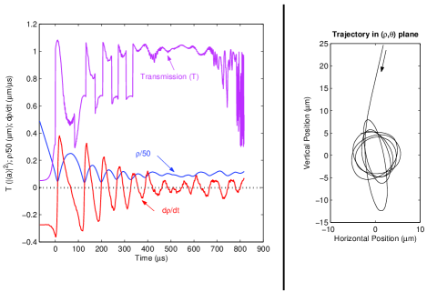
Figure 6: Simulated feedback example with perfect sensing of $\rho(t)$. The graph on the left shows idealized cavity transmission $T(t)$ (purple), radial position $\rho(t)$ (blue), and $d\rho/dt$ (red) for a simulated atom trajectory. In the right panel the same atomic trajectory is shown in the $(x,y)$ (or $(\rho,\theta)$) plane. This trajectory begins as a nearly vertical transit through the cavity, but is circularized by the feedback employed. In the left panel, the circularization is evident as $d\rho/dt$ is damped towards zero and $\rho$ and $T$ become nearly constant at the end of the trajectory.

A 10-$\mu$s box filter is applied to $\dot{\rho}$ in order to remove some oscillations caused by $x$ motion and also partially to anticipate some effects of noisy detection and delay. In setting the conditions for potential-switching, we employ the asymmetric hysteresis described above with $(lim,\delta)$=(0.05,0.03)$\mu$m$/\mu$s, so the potential depth is switched at $\dot{\rho}=+0.05,-0.08\mu$m$/\mu$s. Switching events, since they correspond to turning the light level up and down, can be seen as sharp edges in the transmitted light $T$. As the example illustrates, the control strategy successfully circularizes atomic trajectories within a few orbital cycles. This can be seen from $\rho(t)$ as well as from the trajectory shown in the $(\rho,\theta)$ plane. The hysteresis limits are chosen so that variations in $\rho$ due only to dynamical noise tend not to trigger any switching of the drive. This is illustrated by the continued high control level throughout the time $t=500-650\mu$s, while $\rho$ is wandering diffusively rather than oscillating with regularity.

The overall trap lifetime is dominated, as in this example, by heating in the $x$ direction. (In the example shown, note the fast, large-amplitude variation in transmission just before the atom escapes; this is a signature of rapid axial heating.) Thus our feedback strategy has little impact (at the level of 10%) on average trapping lifetimes. Circularizing the orbit helps decrease axial heating since the potential depth no longer wanders as $\rho$ varies; however, the feedback is accomplished by sharp switching events which occur at arbitrary times relative to the oscillations in the $x$ direction. The overall impact on lifetimes is therefore small in the simulations we have performed. Since the feedback algorithm is aimed at reducing motion in the $\rho$ direction, its success is best measured by its performance at that task specifically. Lifetime effects can become apparent only if the axial motion is suppressed by some other means; that case is treated briefly in Section E below.

IV.2 Adding Measurement Noise Adds Delays

The addition of measurement noise and consequent estimation of $\dot{\rho}$ introduce significant loop delays, as described above. Since $\dot{\rho}_{est}$ can be almost half a cycle behind the actual $\dot{\rho}$, we expect naive switching to be well out of phase with the atomic motion and thus relatively ineffective as a cooling mechanism. Figure 7 shows an example in which the feedback strategy is identical to that of Figure 6, but applied to $\dot{\rho}_{est}$ rather than to $\dot{\rho}$ itself. The resulting time delay seriously compromises performance, as shown. In the figure, note that the switching events, recognizable as sharp edges in transmission, do not line up with turning points of $\rho$. As a result, $\dot{\rho}$ is not damped and the trajectory remains elliptical.

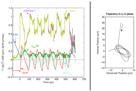
Figure 7: Measurement noise leads to filtering and unacceptable loop delay in this example. In addition to the quantities plotted in Figure 6, the left panel now displays the experimentally realistic transmission $T(t)$ with noise (yellow), and the radial motion estimators $\rho_{est}(t)$ (green) and $(d\rho/dt)_{est}$ (light blue) arising from the noisy transmission signal. Feedback switching is triggered by the value of $(d\rho/dt)_{est}$, but since the estimator lags well behind the true $d\rho/dt$ damping is not achieved, and indeed the two-dimensional trajectory shows little change in shape over time.

IV.3 Account for Delays by Waiting a Cycle

Since it seems clear we cannot simply close the loop with the delays necessitated by measurement noise, we choose to address the problem by adding even more delay – that is, by detecting a switching condition ($\dot{\rho}_{est}$ crossing a hysteresis limit) and then waiting to switch the potential at a time which should catch the next oscillation of $\rho$. A first attempt in this direction would be to assume a fixed period for oscillations of $\rho$. In this case the additional wait before switching is given by this fixed period minus the estimator delay for $\dot{\rho}_{est}$. Since each switching time is now set by the detected signal from the previous cycle, the first switching opportunity (first minimum of $T$ and maximum of $\rho$) will be missed in this strategy. Rather than miss this cooling cycle, we impose a single switching event a fixed time after the initial trap turn-on. Thus the potential switches exlo$\rightarrow$hi on the initial trigger, hi$\rightarrow$lo a fixed time later, and lo$\leftrightarrow$hi thereafter based on the last zero-crossing time of $\dot{\rho}_{est}$.

However, the actual dynamical period varies by easily a factor of two over the course of an atom’s trapping lifetime due to changing amplitude of oscillation in the anharmonic potential, as seen in Figure 3b. Thus the fixed-period assumption is a poor one. A better strategy is to record the length of each period in $\dot{\rho}_{est}$ and assume each cycle will be the same length as the previous recorded one. Thus the “waiting time” estimate will adjust itself as the dynamical period changes, though it will in general be one cycle behind. This strategy is employed for the trajectory shown in Figure 8. The initial switch occurs 45$\mu$s after trap turn-on, the least-squares window is 40$\mu$s, and the “wait time” between subsequent $\dot{\rho}_{est}$ limit-crossings and the resultant potential switches is given by the previous period minus 20$\mu$s. This switching strategy, with deliberate delay based on an active measurement of the $\rho$ oscillation time, appears to be a viable means of performing control in the presence of sensor noise and its associated loop delay.

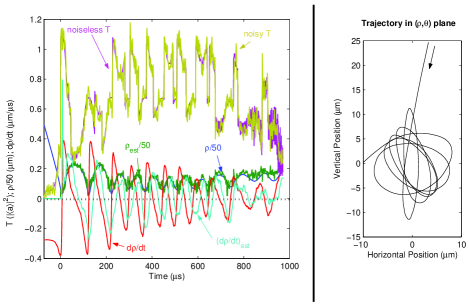
Figure 8: In this example delay is dealt with by tracking $\rho$ turning points and using this information from each cycle to switch the potential at the predicted next turning point. This strategy give moderate success at damping $d\rho/dt$ and circularizing the trajectory.

IV.4 Comparisons with Open Loop Strategies

To evaluate the effects of feedback more quantitatively, we introduce a figure of merit for the damping of radial oscillations in an atomic trajectory. Since the goal of the control strategy is to confine $\dot{\rho}$ near zero, the performance can be measured by comparing the variance of $\dot{\rho}$ over intervals of equal duration near the beginning of the trajectory and after feedback has been operating for some time. We choose a time window of duration 200$\mu$s as long enough to encompass well over one cycle of the radial motion. The comparison is taken between two such windows separated from one another by 200$\mu$s; this delay is selected as long enough for several cycles of feedback action, yet short enough so that the statistic exists for a large fraction of trapped atom events. Finally, we base our performance measure on the experimentally accessible $\dot{\rho}_{est}$ rather than on $\dot{\rho}$ itself. Thus our figure of merit for feedback performance is given by

$$M=\frac{\sigma^{2}_{15\mu s\rightarrow 215\mu s}(\dot{\rho}_{est}(t))}{\sigma^{2}_{415\mu s\rightarrow 615\mu s}(\dot{\rho}_{est}(t))}$$ (8)

where times are measured from the initial trapping (exlo$\rightarrow$hi) switch. Large values of the quantity $M$ correspond to well-damped radial motion, $\rho(t)\rightarrow constant$, though orbits may still be circular at any radius $\rho\geq 0$. (Damping in the sense of actual energy removal is discussed explicitly in Section E.) Small ($\sim 50-100\mu s$) changes in delay time or window size have been investigated and do not appreciably change the nature of the results for $M$.

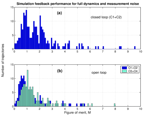
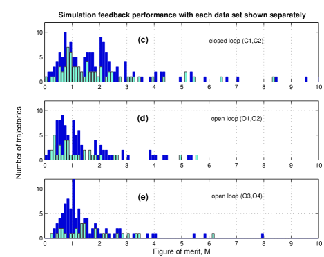
Figure 9: Figure of merit for feedback in closed- and open-loop cases (full dynamics). $M>$1 indicates damping of radial motion.

Figure 9 shows histograms of $M$ for several data sets in which different switching protocols, detailed in Table 1, have been employed. Each data set is generated by simulating a fixed number of individual atom drops from the known distribution of initial conditions. Only some fraction of trajectories result in a triggering/trapping event, and of these only a fraction of atoms have dwell times long enough to compute a value for $M$. Thus, for example, set C2 was generated from 5,000 trajectories, yielding 1,335 trigger events and 147 trajectories for which $M$ could be obtained (i.e., with dwell times at least 615$\mu$s).

Data set	switching protocol	# atom drops	# trapped
C1	Closed loop	2000	534
	Switch once
	45 $\mu$s after
	initial trigger.
	Thereafter switch
	(previous cycle length)
	- 20$\mu$s after
	$(d\rho/dt)_{est}$
	crosses limits.
C2	Same as above (C1)	5000	1335
O1	Open loop	2000	561
	Switch every 45$\mu$s
	after initial trigger.
O2	Same as above (O1)	5000	1319
O3	Open loop	2000	552
	Switch every 35$\mu$s
	after initial trigger.
O4	Same as above (O3)	5000	1322

Table 1: Exact conditions used for data of the full-simulation histograms.

While Table 1 gives the specifics of each data set represented in Figure 9, the essential comparison is between closed loop – i.e., active feedback – algorithms and open loop counterparts which simply switch potentials in a predetermined sequence independent of real-time position information for the individual atom. The closed loop algorithm is that of Figure 8, in which measurement noise and loop delays are dealt with by waiting nearly one cycle to apply the knowledge of motion gained during the previous oscillation. The open loop algorithms, in contrast, simply switch the potential between hi and lo at fixed intervals following the initial trapping event; the fixed interval is chosen to coincide with a reasonable average value for an atomic oscillation period. Over a long atomic trajectory, the atomic trajectory clearly evolves out of phase with any one open loop switching algorithm; since this evolution is different for each atomic trajectory, we compare closed-loop with open-loop strategies as a means of evaluating the importance of real-time measurement and feedback in our algorithm.

Closed loop, active feedback clearly damps radial oscillations more effectively than its open loop counterpart. The $M$ distributions in Figure 9(a,c) have larger mean than those in Figure 9(b,d,e), with the closed-loop histograms showing many trajectories pushed out to higher values of $M$ by the active feedback. These results indicate that real-time measurements of $\rho(t)$ can indeed be applied to facilitate cooling of a single atom’s motion in that dimension.

Further refinements should improve the performance of the algorithm. For instance, the cycle-length predictor could be changed to allow asymmetries between $\dot{\rho}>0$ and $\dot{\rho}<0$ half-cycles. Additionally, the filters themselves could be adjusted or replaced with better estimators which incorporate information about angular momentum $L$.

The simulations reported here could in principle be employed, with minor modifications, to address the experimental regime of the atom-cavity feedback performed in Ref. rempefb . We have not attempted a quantitative comparison since results may be sensitive to details of the experimental implementation. However, we note that because of the values of $(g,\kappa)$ for the optical cavity employed, Ref. rempefb was carried out in a qualitatively different regime from the one in which our simulations operate. In particular, while both scenarios involve a measurement bandwidth which averages over axial motion, in the case of Ref. rempefb the amplitude of the axial motion is in fact quite large. One key observation in that experimental setting was in fact the change in measured transmission as atoms either oscillated within a single standing-wave antinode or “flew” across multiple antinodes. Without the measurement bandwidth to observe axial oscillations directly, one is hard pressed to separate axial modulation from radial motion in the manner presented here. While both feedback algorithms involve a similar switching of cavity driving strength, the feedback modeled here is directed at cooling a particular component of the atom’s motion $\vec{r}(t)$. Figures 9 and 10 illustrate the damping of $d\rho/dt$. By contrast, the lifetime enhancement of Ref. rempefb occurs because the authors are able to discern when the atom is trapped at high $g(\vec{r})$ and selectively turn down the otherwise large diffusive heating by lowering the trap intensity at those times.

IV.5 Performance with Axial Motion Suppressed

In a final set of simulations, we investigate the performance of our radial cooling algorithm in a setting where the axial atomic motion is independently suppressed. With no (or little) axial motion, axial heating no longer limits trapping times and the effects of radial feedback can be seen more clearly. To achieve this in simulations, we impose an ad hoc elimination of the axial dimension; however, this case could be relevant to several future experimental scenarios. For example, trapping and sensing mechanisms, both currently accomplished with the same probe beam, could be separated to allow a trapping field with a low scattering rate and much-reduced axial diffusion. Alternatively, the separation of axial and radial timescales could be exploited, either to apply axial coolingstevencooling between cycles of radial feedback or to simply avoid extra axial heating by ramping the potentials up and down at a rate that appears adiabatic to the axial motion while still impulsive in the radial dimension.

Prospects for implementation aside, simulations with no axial motion demonstrate some aspects of the radial feedback protocol that are otherwise less transparent. We explore this regime with a set of simulations that differ in three ways from those presented above. First, the axial dimension is eliminated entirely and the atom is artificially constrained to remain at rest at an antinode of the standing-wave cavity field. Second, since axial heating is no longer an issue, we employ somewhat deeper trapping potentials than in the simulations above. The weak probe level is still $n_{exlo}=0.05$ photons in the empty cavity, but now we turn on the trap initially at a level $n_{exhi}=0.6$ photons in the empty cavity, and we feed back by switching between this and the weaker level $n_{hi}=0.3$ photons. The effective potentials thus generated are $\sim 50\%$ deeper than in the previous simulations using $n_{hi}$ and $n_{lo}$. Finally, without axial motion we employ a coarser computational timestep of (1/30)$\mu$s.

Figure 10(a) shows the feedback figure of merit for the cases of closed-loop feedback, constant trapping at $n_{hi}$ or $n_{exhi}$, and open-loop switching. The open-loop protocol in this case is to trap initially with $n_{exhi}$ and switch between driving levels $n_{exhi}$ and $n_{hi}$ every 40$\mu$s during the transit duration. Taking advantage of longer overall atom dwell times, we can now consider time windows separated by a greater delay, so the quantity displayed here is

$$M^{\prime}=\frac{\sigma_{15\mu s\rightarrow 215\mu s}^{2}(\dot{\rho}_{est}(t))}{\sigma_{1015\mu s\rightarrow 1215\mu s}^{2}(\dot{\rho}_{est}(t))}$$ (9)

rather than the original $M$ of Figure 9. The result is qualitatively similar to that of the full simulation, with the closed loop strategy performing significantly better than its open loop counterpart. In this case, the mean value of $M^{\prime}$ for closed-loop feedback is $\sim 2.5$ times greater than for open-loop switching or for no switching.

(a)

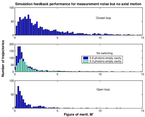
(b)

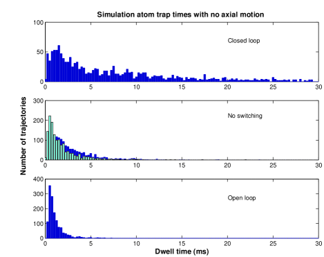
Figure 10: Feedback performance and lifetime enhancement in simulations with no axial motion. $M^{\prime}>$1 indicates damping of radial motion.

The data of Figures 9 and 10(a) indicate that our feedback algorithm acts to drive $\dot{\rho}$ to zero, i.e., to circularize atomic orbits at a constant value of $\rho$. If angular momentum $L$ is not correspondingly increased, this effect implies a damping of radial energy. However, we may investigate more directly whether this algorithm actually removes total energy from the radial motion. With axial motion eliminated, we can now explore this issue by asking how the feedback algorithm affects trapping lifetimes. Figure 10(b) shows atom dwell times for the same three cases of closed-loop feedback, constant drive levels of $n_{exhi}$ or $n_{hi}$, and open-loop switching. The increase in lifetime for closed-loop feedback is immediately apparent. Indeed, the closed-loop results agree well with an exponential lifetime of 8.9ms, as contrasted with 2.6ms for trapping at $n_{exhi}$ alone, 1.9ms for trapping at $n_{hi}$, and 1.1ms for open-loop switching between the drive levels.

In the closed-loop case the trap potential is varied during the transit but never exceeds the depth associated with driving level $n_{exhi}$. Nevertheless, trap times exceed those for constant driving at $n_{exhi}$, demonstrating that active feedback as applied to the radial dimension does act to remove radial energy, in addition to simply pinning $\rho$ to a constant value. The same point can be illustrated by considering the change in total energy between the beginning (15-215 $\mu$s after trigger) and end (1015-1215 $\mu$s after trigger) of an atom’s dwell time in the cavity; the active feedback strategy produces a modest ($\simeq$10%) net energy removal not seen under either the simple trap or the open-loop switching protocol. Since the feedback algorithm performs better than both open-loop and fixed-trap strategies when measured by dwell time, radial damping $M^{\prime}$, or total energy removal, we characterize its effect as in fact actively cooling a component ($\rho(t)$) of the atomic motion.

Note that all lifetime in the two-dimensional simulation are enhanced relative to the full three-dimensional case, in which both experiments and simulations have mean trapping times of only $\sim 400\mu$s. Lack of lifetime enhancement from radial feedback in the full simulation is some indication of the very weak mixing between axial and radial motion, so that cooling in one of these dimensions does little to control temperatures in the other.

V Outlook for Experimental Implementation

The feedback simulations discussed in this paper have been conducted with very close reference to the conditions realized in the experiment of Ref. acm , in particular for cavity properties, trapping statistics, and signal-to-noise in the balanced heterodyne detection. The current experimental effort, aimed at realizing the feedback strategies described here, employs very similar conditions while incorporating some improvements as in Ref. fort ; mckeever ; mcknature . Notable changes from Ref. acm include a slightly shorter cavity, improved vacuum pressure in the cavity region ($3$x$10^{-10}$ torr) enabled by a differentially pumped double chamber, and cavity length stabilization via an error signal generated by an independent laser one free spectral range away from the cavity QED light. Implementation of the feedback strategy described above is clearly outside the regime of analog electronics, so an additional modification is the use of digital processing and FPGA technologyfpga . With these tools, experimental data similar to the simulation results presented above seem well within reach.

It seems reasonable to ask how much experimental data should be necessary to exhibit a distinction between active feedback and open loop schemes. From the simulations of Figure 9 (Table 1), we see that with data sets of about 500 trapped atoms the differences between open- and closed-loop schemes already begin to become apparent, and these differences are well demarcated with two or three times that much data. With fairly conservative estimates of one trigger per MOT drop and one MOT drop every 5 seconds, this means significant effects could well be seen with just one to two hours of experimental data at each setting. Much more data collection is experimentally realistic, allowing exploration of a wealth of additional questions.

With the atom-cavity system’s capacity to give real-time information on a trapped atom’s position, active feedback might seem to be an attractive enabling technology for experiments that require a stationary atom at fixed $g(\vec{r})$ in the cavity field. The present work was undertaken in part to explore this option through simulation of realistic experiments. While we conclude that feedback of a uniquely real-time nature can measurably alter properties of the atomic motion, we also find that measurement bandwidths and signal to noise strongly constrain the precision of feedback performance under current experimental conditions. Feedback experiments address important topics in quantum measurement and control; meanwhile, trapping strategies using auxiliary fields offer a more direct route towards a stationary atom in a cavity.

VI Current Limits and Future Directions

The feedback algorithm developed above for the atomic radial position $\rho$ is subject to basic limits arising from dynamical and measurement noise in our system. These limits can be expressed as lower bounds on the (one-dimensional) temperature for $\rho$. Because the strategy is based on discrete switching, with feedback delayed and timed based on the previous switching-cycle length, the control is always based on information gathered over the previous motional cycle. Thus dynamical noise over an atomic motional timescale will set a lower limit on $T_{\rho}$. Referring to acdpra , we find that momentum diffusion (due to spontaneous emission) gives a typical energy increase per radial oscillation time of $\Delta E_{\tau_{r}}\sim 0.02(U_{0})\sim k_{B}(50\mu K)$. Furthermore, measurement noise places a limit on the detectable amplitude of $\rho$ variations. This amplitude depends strongly on the absolute value of $\rho$ due to the nonlinearity of the $T\rightarrow\rho$ mapping. However, using the measured sensitivity from the atom-cavity microscope, we estimate that over a motional cycle we can resolve $\rho$ oscillations of amplitude $(20nm/\sqrt{Hz})\sqrt{1/2\pi\tau_{r}}\approx 0.77\mu m$. On the side of the cavity mode, where the effective potential is steepest, this corresponds to $T_{\rho}\approx 150\mu K$. While this limit corresponds closely to the simulations of the previous section, where axial motion is suppressed, the full simulation never reaches this limit because axial heating cuts off atomic lifetimes too quickly. Thus improvements to address axial heating are of great interest for seeing the full effect even of radial cooling.

Beyond the experimental and algorithmic variations already discussed, a number of broader questions are raised by the use of active feedback to dynamically cool a component of motion for a single atom. One question deals with the ultimate limits of such a cooling mechanism. Within the current experimental setting, limits to radial cooling arise from atomic lifetimes (dominated by axial motion), but are also constrained by the dynamical noise and by the shot noise of detection. Some lifetime and dynamical noise issues could be addressed by separating trapping and sensing, for example by using a far off resonance trap in conjunction with a sub-photon level cavity QED probemckeever . The remaining issues would then center on signal-to-noise for the atomic position measurement, as well as on limits imposed by backaction of the measurement itself as it approaches the standard quantum limitsql ; gambetta . These limits must be considered not only in the context of near-resonant probing, as treated here, but also in the case of a far detuned probe for which atomic position information is extracted from probe phase shifts, as first measured in fullmeas .

Extension of active feedback beyond the $\rho$ dimension raises related questions. The question here is one of using various techniques – for example, a symmetry-breaking potential as could be provided by a higher-order transverse mode of the cavity or frequency-domain filtering of the signal – to estimate and control a three-dimensional vector using the time record of a single quantity, the transmitted light field. Undoubtedly, different driving parameters, detection methods, and data processing will be appropriate depending on the relative importance placed on information about each dimension of the motion. These questions address in various ways some basic issues of optimal state estimation and control for single quantum systems, and this experimental system promises to be a rich one for exploring such issues in further detail.

- [1] C. J. Hood, T. W. Lynn, A. Doherty, A. S. Parkins, and H. J. Kimble. Science, 287:1447, 2000.
- [2] P. W. H. Pinkse, T. Fischer, P. Maunz, and G. Rempe. Nature, 404:365, 2000.
- [3] J. Ye, D. W. Vernooy, and H. J. Kimble. Phys. Rev. Lett., 83:4987, 1999.
- [4] J. McKeever, J. R. Buck, A. D. Boozer, A. Kuzmich, H.-C. Naegerl, D. M. Stamper-Kurn, and H. J. Kimble. Phys. Rev. Lett., 90:133602, 2003. Available as quant-ph/0211013.
- [5] J. McKeever, A. Boca, A. D. Boozer, J. R. Buck, and H. J. Kimble. Nature, 425:268, 2003.
- [6] P. Maunz, T. Puppe, I. Schuster, N. Syassen, P. W. H. Pinkse, and G. Rempe. Nature, 428:50, 2004.
- [7] A. C. Doherty, T. W. Lynn, C. J. Hood, and H. J. Kimble. Phys. Rev. A, 63:013401, 2001. Available as quant-ph/0006015.
- [8] J. I. Cirac, S. J. van Enk, P. Zoller, H. J. Kimble, and H. Mabuchi. Phys. Scripta, T76:223, 1998.
- [9] T. Pellizzari, S. Gardiner, I. Cirac, and P. Zoller. Phys. Rev. Lett., 75:3788, 1995.
- [10] J. I. Cirac, P. Zoller, H. J. Kimble, and H. Mabuchi. Phys. Rev. Lett., 78:3221, 1997.
- [11] S. J. van Enk, J. I. Cirac, and P. Zoller. Science, 279:205, 1998.
- [12] H. J. Briegel, W. Dur, J. I. Cirac, and P. Zoller. Phys. Rev. Lett., 81:5932, 1998.
- [13] H. J. Briegel, S. J. van Enk, J. I. Cirac, P. Zoller, in The Physics of Quantum Information, D. Bouwmeester, A. Ekert, A. Zeilinger, Eds. (Springer, Berlin, 2000), pp. 192-197.
- [14] E. T. Jaynes and F. W. Cummings. P. IEEE, 51:89, 1963.
- [15] J. J. Sanchez-Mondragon, N. B. Narozhny, and J. H. Eberly. J. Opt. Soc. Am. B, 1:518, 1984.
- [16] C. J. Hood, M. S. Chapman, T. W. Lynn, and H. J. Kimble. Phys. Rev. Lett., 80:4157, 1998.
- [17] T. Fischer, P. Maunz, P. W. H. Pinkse, T. Puppe, and G. Rempe. Phys. Rev. Lett., 88:163002, 2002.
- [18] JM Geremia, J. K. Stockton, and H. Mabuchi. Science, 304:270, 2004.
- [19] H. Mabuchi. Phys. Rev. A, 58:123, 1998.
- [20] H. Mabuchi, J. Ye, and H. J. Kimble. Applied Phys. B, 68:1095, 1999.
- [21] A. Soklakov and R. Schack. quant-ph/0210024, 2002.
- [22] J. Gambetta and H. M. Wiseman. Phys. Rev. A, 64:042105, 2001.
- [23] H. J. Kimble. Phys. Scripta, T76:127, 1998.
- [24] C. Cohen-Tannoudji, J. Dupont-Roc, and G. Grynberg. Atom-Photon Interactions. Wiley, New York, 1992.
- [25] H. J. Carmichael. Statistical Methods in Quantum Optics 1. Texts and Monographs in Physics. Springer-Verlag, Heidelberg, 1st edition, 1999.
- [26] S. M. Tan. J. Opt. B: Quant. Semiclass. Opt., 1:424, 1999.
- [27] D. A. Steck, K. Jacobs, H. Mabuchi, T. Bhattacharya, and S. Habib. quant-ph/0310153, 2003.
- [28] O. L. R. Jacobs. Introduction to Control Theory. Oxford University Press, New York, 1993.
- [29] A. C. Doherty. PhD thesis, The University of Auckland, 1999.
- [30] Lee Barford, Eric Mandres, Gautam Biswas, Pieter Mosterman, Vishnu Ram, and Joel Barnett. Technical Report HPL-1999-18, Integrated Solutions Laboratory, HP Laboratories, Palo Alto, CA, February 1999. Available at www.hlp.hp.com/techreports/1999/HPL-1999-18.html.
- [31] O. Vainio, M. Renfors, and T. Saramaki. IEEE Trans. Inst. Meas., 46:5, 1997.
- [32] S. J. van Enk, J. McKeever, H. J. Kimble, and J. Ye. Phys. Rev. A, 64:013407, 2001. Available as quant-ph/0005133.
- [33] J. Stockton, M. Armen, and H. Mabuchi. J. Opt. Soc. Am. B, 19:3019, 2002.