Differential atom interferometry beyond the standard quantum limit

Abstract

We analyze methods to go beyond the standard quantum limit for a class of atomic interferometers, where the quantity of interest is the difference of phase shifts obtained by two independent atomic ensembles. An example is given by an atomic Sagnac interferometer, where for two ensembles propagating in opposite directions in the interferometer this phase difference encodes the angular velocity of the experimental setup. We discuss methods of squeezing separately or jointly observables of the two atomic ensembles, and compare in detail advantages and drawbacks of such schemes. In particular we show that the method of joint squeezing may improve the variance by up to a factor of 2. We take into account fluctuations of the number of atoms in both the preparation and the measurement stage, and obtain bounds on the difference of the numbers of atoms in the two ensembles, as well as on the detection efficiency, which have to be fulfilled in order to surpass the standard quantum limit. Under realistic conditions, the performance of both schemes can be improved significantly by reading out the phase difference via a quantum non-demolition (QND) measurement. Finally, we discuss a scheme using macroscopically entangled ensembles.

I I. Introduction

Comparing the phase shifts obtained in two independent interferometric setups has several applications, prominent examples being the comparison of atomic clocks atomicclocks , and Sagnac interferometry to discriminate between rotations and accelerations jentsch . In addition, the comparison of gravitational forces at different points in space or for different atomic species weitz allows to test predictions of possible violations of Einstein’s general relativity snadden:1998 ; kasevich:2002 . For such differential interferometers, the quantity of interest is encoded in either the difference, or the sum of the individual phase shifts.

Especially for the measurement of inertial forces, atom interferometers promise high resolution. Here atom optical elements like beam splitters and mirrors can be realized using Raman transitions between two atomic ground state levels KasevichChu . The accumulated phase difference between the interferometer paths is encoded in the number difference of atoms in the exit ports labeled by different internal states. For example, this can be measured by state selective fluorescence detection. Such schemes have already been successfully implemented to measure inertial forces and the earth’s gravity with a high accuracy KasevichChu ; peters . In Sagnac atom interferometry, the goal is to measure the phase shift which occurs when the laser setup (laboratory frame) is rotating relative to the frame of the freely flying atomic ensembles. This phase shift is given by $\phi^{\rm at}=4\pi{\bf A}\;\mbox{\boldmath$\Omega$}\;m_{\rm at}/h$ as compared to $\phi^{\rm light}=4\pi{\bf A}\;\mbox{\boldmath$\Omega$}/(\lambda c)$ for laser interferometers, where $m_{\rm at}$ is the mass of the atoms, ${\bf A}$ is the oriented enclosed area of the interferometer, $\Omega$ is the vector of angular velocity, and $\lambda$ is the wavelength of the light. For an atomic gyroscope working with ⁸⁷Rb, the phase $\phi^{\rm at}$ is $10^{11}$ times larger than the corresponding phase $\phi^{\rm light}$ of a light interferometer enclosing the same area and operating at $\lambda=10^{3}\;$nm. Hence, atom interferometers promise an enormously improved resolution for rotation measurements as compared to “classical” photonic devices.

The Sagnac phase can be measured by letting two ensembles of atoms pass through the interferometer from opposite sides. They obtain then phase shifts $\pm\phi$ due to the rotation of the laboratory frame, where the sign depends on the direction of propagation of the ensembles, and a common phase shift $\theta$ due to effects such as an acceleration of the setup. Subtracting the phases of the two ensembles yields the desired phase $2\phi$, which encodes the rotation of the setup around an axis perpendicular to the plane of the interferometer. Collisions between the two ensembles in the interferometer can safely be neglected due to the low atomic densities of the ensembles.

In the standard quantum limit for phase measurements in atomic interference experiments, the variance of the phase due to quantum projection noise is given by $(\Delta\phi)^{2}_{\rm SQL}=1/N,$ where $N$ is the number of atoms in a sample. By feeding the interferometer with non-classical states of atoms, the so-called squeezed states, this limit can be surpassed, with a fundamental bound given by $(\Delta\phi)^{2}_{\rm H}=1/N^{2},$ the so-called Heisenberg limit inter ; heisenberg ; oblak . Squeezed atomic states can be produced by a quantum non-demolition (QND) interaction of the atoms with a light beam QND , or by absorption of non-classical states of the light absorbnonclassical . Squeezed states of atomic ensembles might also be useful as quantum memory for states of light memory .

It has been shown that for such squeezed states atoms within an ensemble are entangled with each other Soerensen . In addition to this entanglement on a microscopic level, it is also possible to entangle macroscopic degrees of freedom of two atomic ensembles with a similar interaction Duan1 ; Polzik . This in principle enables teleportation of the macroscopic state of an ensemble. Furthermore, it has been shown recently that such macroscopically entangled ensembles can improve the efficiency of measurements of the components of a magnetic field Vivi . Here, we try to exploit microscopic as well as macroscopic entanglement between two atomic ensembles in the context of differential interferometry, where we focus especially on an atomic Sagnac interferometer setup.

In Section II we calculate the phase variance for a differential interferometer using non-squeezed coherent states in order to introduce our methodology. We show also how to include number fluctuations into the calculations. These will turn out to be important later. In Section III we show that the phase uncertainty can be reduced by feeding the interferometer with individually squeezed ensembles. In Section IV we consider squeezing of a joint observable of both ensembles. In Section V we discuss how decoherence affects the interferometer, and in Section VI we compare the variances of the schemes discussed so far for realistic parameters. Finally, in Section VII the use of macroscopically entangled states in the interferometer is discussed.

II II. Coherent input states

For a single atom we define a pseudo spin-$1/2$ through two ground state atomic hyperfine levels $|1\rangle$ and $|2\rangle$ jentsch ; kasevich:2002 by introducing the relevant spin operators as

$$\hat{\sigma}_{z} = \frac{1}{2}\left(|1\rangle\langle 1|-|2\rangle\langle 2|\right)\;,\quad\hat{\sigma}_{x}=\frac{1}{2}\left(|1\rangle\langle 2|+|2\rangle\langle 1|\right)\>,$$

$$\hat{\sigma}_{y} = \frac{1}{2i}\left(|1\rangle\langle 2|-|2\rangle\langle 1|\right).$$ (1)

We will subsequently only consider the collective spin $\hat{\bf J}=\sum_{i=1}^{N_{J}}\hat{\mbox{\boldmath$\sigma$}}{\,(i)}$ for the first, and in analogy $\hat{\bf L}$ for the second ensemble; $N_{J,L}$ are the number of atoms in the ensembles $J$ and $L$, respectively. The measurements that can typically be performed in atom interferometry are population measurements of the levels $|1\rangle$ and $|2\rangle$ by fluorescence techniques Kasevich . Hence, only the $z$ components of the collective spin vectors can be measured directly.

II.1 II.A. Description of the interferometer

Initially, all the atoms are assumed to be prepared in the state $|1\rangle$, leading to the following expectation value and variance of the collective spin vector:

$${\langle\hat{\bf J}\rangle}=\frac{N_{J}}{2}\hat{\bf z},\quad(\Delta\hat{J}_{z})^{2}=0,\quad(\Delta\hat{J}_{x,y})^{2}=\frac{N_{J}}{4},$$ (2)

Analogous values are obtained for the ensemble $\hat{\bf L}$. Corresponding to the definitions in Eq. (II), the $z$ axis denotes the difference of the number of atoms in states $|1\rangle$ and $|2\rangle$, whereas the phase difference between these two states is encoded in the $x-y$ plane. The uncertainties stem from the single particle uncertainties, and correspond to a state with a fixed number of atoms.

A typical interferometer sequence used for the measurement of inertial forces consists of three atom–light interactions as shown in Fig. 1. The first beam splitting Raman pulse transfers all the atoms from the ground state $|1\rangle$ to the superposition $\frac{1}{\sqrt{2}}(|1\rangle+|2\rangle)$. Atoms transfered to state $|2\rangle$ obtain a momentum kick of two photon recoil if the two Raman lasers are counter-propagating, so that the partial waves delocalize, as depicted in Fig. 1. The second pulse exchanges the populations, $|1\rangle\leftrightarrow|2\rangle$, and deflects the partial waves. Finally, they are recombined in the last interaction zone, acting as a beam splitter.

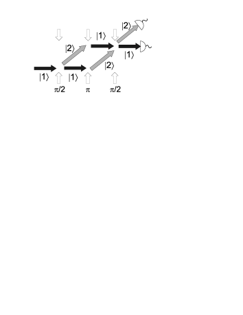
Figure 1: Scheme of the atom interferometer. $\frac{\pi}{2}$ and $\pi$ label the beamsplitting and the mirror pulses, respectively. The populations in the two exit ports are detected state-selectively via fluorescence measurements.

These pulses can be represented as rotations of the collective spin vectors ${\langle\hat{\bf J}\rangle}$ and ${\langle\hat{\bf L}\rangle}$ around an axis in the $x-y$ plane, the angle being given by $\pi/2$ for beam splitters and by $\pi$ for mirrors. For a fixed coordinate system the angle between the $x$ axis and the rotation axis is given by the laser phase atominterferometry . The laser phases change if the setup (laboratory frame) rotates with respect to the path of the freely flying ensembles, which causes the Sagnac phase shift. This change corresponds to a rotation of the collective spin vectors in the $x-y$ plane around the $z$ direction.

In order to make the scheme applicable to a more general scenario for differential interferometers, we model it as follows for each of the ensembles labeled by $\hat{\bf J}$ and $\hat{\bf L}$, respectively: the first beam splitter rotates each collective spin vector by $\pi/2$ around the $y$ axis, then we collect all the phase shifts occurring in the interferometer in rotations around $z$ of $\hat{{\bf J}}$ and $\hat{{\bf L}}$ by $\Phi_{J}$ and $\Phi_{L}$, respectively. Finally, a $\pi$ and a $\pi/2$ pulse, both around $x$, implement the mirror and the final beam splitter, respectively. These last two pulses can be combined to a single rotation around the $x$ axis by $-\pi/2$.

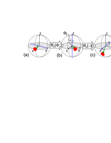
Figure 2: (Color online) Interferometric scheme for a coherent input state: (a) collective spin after the first beam splitter, (b) the total phase $\phi$ accumulated in the interferometer results in a rotation around $z$, before (c) a final rotation around $x$ by $-\pi/2$ implements the mirror and the final beam splitter, encoding the phase in the $z$ direction.

All relevant interferometric steps are described in Fig. 2, where the atomic spin vector is depicted together with a disc representing the corresponding uncertainties of the spin operators. To simplify notation we will take the state after the first beam splitter as the initial state: $\hat{{\bf J}}^{\rm in}={\cal R}_{y}(\pi/2)\hat{{\bf J}}$, see Fig. 2(a). Here ${\cal R}_{i}(\alpha)$, $i\in\{x,y,z\}$, is the matrix rotating a vector by the angle $\alpha$ around the direction $\hat{\bf e}_{i}$. In the Heisenberg picture, and neglecting collisions between the atoms within the ensemble, the spin operator changes according to $\hat{{\bf J}}^{\rm out}={\cal R}_{x}(-\pi/2){\cal R}_{z}(\Phi_{J})\hat{{\bf J}}^{\rm in}$. This leads to

$$\hat{{\bf J}}^{\rm out}=\left(\begin{array}[]{c}\hat{J}_{x}^{\,\rm in}\cos\Phi_{J}-\hat{J}_{y}^{\,\rm in}\sin\Phi_{J}\\ \hat{J}_{z}^{\rm in}\\ -\hat{J}_{x}^{\,\rm in}\sin\Phi_{J}-\hat{J}_{y}^{\,\rm in}\cos\Phi_{J}\end{array}\right).$$ (3)

It is also possible to consider a balanced atom interferometer in which all rotations are around the $x$ axis. In this case, an extra $\pi/2$ shift around $z$ leads to the same result. The advantage of the extra pulse is that for the initial state of Eq. (2)

$${\langle\hat{J}_{z}^{\rm out}\rangle}=-\frac{N_{J}}{2}\sin\Phi_{J}\approx-\frac{N_{J}}{2}\Phi_{J}$$ (4)

for small angles $\Phi_{J}$, while with the unmodified balanced scheme ${\langle\hat{J}_{z}^{\rm out}\rangle}$ would be proportional to $\cos\Phi_{J}$, and hence sensitive to $\Phi_{J}$ only in second order around $\Phi_{J}=0$.

As explained in the introduction, the phase will be given by $\Phi_{J}=\phi+\theta$ for $\hat{\bf J}$ and by $\Phi_{L}=-\phi+\theta$ for $\hat{\bf L}$, because the Sagnac phase $\phi$ takes a different sign, depending on direction in which the ensemble passes the interferometer. We define the phase operator for the case of coherent states (cs) as

$$\hat{\phi}_{\rm cs}=-\frac{\hat{J}_{z}^{\rm out}}{N_{J}}+\frac{\hat{L}_{z}^{\rm out}}{N_{L}}$$ (5)

and obtain to the first order in $\phi$ and $\theta$

$${\langle\hat{\phi}_{\rm cs}\rangle} = \phi$$ (6)

$$(\Delta\hat{\phi}_{\rm cs})^{2} = \frac{1}{4N_{J}}+\frac{1}{4N_{L}}.$$ (7)

The variance of $\hat{\phi}_{\rm cs}$ corresponds to the standard quantum limit. Note that $\theta$ can be obtained in an analogous way. From the definition it is obvious that determining the number of atoms is important for the calculation of the phase shift. A major source of error will come from fluctuations in the number of atoms of the ensembles and hence we will discuss how to include this process into the calculations in the next section.

II.2 II.B. Number fluctuations

There are two sources of deviations of the number of atoms: the preparation process and the number measurement process. The atomic ensembles produced from the source are best described as a statistical mixture of states with different atom numbers, but we will assume that the final number measurement projects onto a number state with $N_{J}$ and $N_{L}$ atoms in the two ensembles. Defining $\bar{N}=(N_{J}+N_{L})/2$, we assume that $|N_{J}-N_{L}|=\gamma\sqrt{\bar{N}}$, which reflects the variances of the number operators $\hat{N}_{J,L}$ of the ensembles after the production. Thus, $\gamma$ is the parameter which describes how well the atom numbers in the two ensembles match.

We treat the number measurements by introducing operators $\delta\hat{N}$ with

$${\langle\delta\hat{N}\rangle}=0,\quad[\Delta(\delta\hat{N})]^{2}=\alpha N,$$ (8)

where $\alpha$ describes the quality of the number measurement. For fluorescence measurements, $\alpha^{-1}$ is given by the mean number of times an atom goes through the fluorescence cycle and scatters a photon which subsequently is registered in the detectors numbers . Typical values in nowadays experiments are $\alpha^{-1}\approx 50\ldots 100$. We replace $N_{J}$ by $N_{J}^{0}+\delta\hat{N}_{J}^{(1)}+\delta\hat{N}_{J}^{(2)}$ and $\hat{J}_{z}^{\rm out}$ by $\hat{J}_{z}^{{\rm out},0}+(\delta\hat{N}_{J}^{(1)}-\delta\hat{N}_{J}^{(2)})/2$. $N_{J}^{0}$ refers to the actual number that would have been measured in perfect number projection measurements, and in $\delta\hat{N}_{J}^{(i)}$ the index $i$ corresponds to the atomic levels $|i\rangle$.

With these substitutions, we obtain

$${\langle\hat{\phi}_{\rm cs}\rangle} = \phi-\alpha\Big{(}\frac{1}{N_{J}^{0}}+\frac{1}{N_{L}^{0}}\Big{)}$$ (9)

$$(\Delta\hat{\phi}_{\rm cs})^{2} = \frac{1}{4N_{J}^{0}}+\frac{1}{4N_{L}^{0}}+\alpha\Big{(}\frac{1}{N_{J}^{0}}+\frac{1}{N_{L}^{0}}\Big{)},$$ (10)

where terms of higher order have been neglected. The contribution from the number fluctuations is in agreement with Ref. numbers . The expectation value of $\hat{\phi}_{\rm cs}$ is shifted for $\alpha\neq 0$. As this shift is of the order of the second term in $(\Delta\hat{\phi}_{\rm cs})^{2}$, it is of second order of the standard deviation only, and can thus safely be neglected. From the expressions it is clear that $\alpha\ll 1$ is required in order to reach the fundamental limit for the phase resolution using coherent input states.

In the following, we will drop the superscript $0$ on the atom number, as long as there is no danger of confusion.

III III. Separately squeezed ensembles

It is known that by taking squeezed input states it is possible to surpass the standard quantum limit in interferometry inter . In this section, we consider the case where both ensembles are squeezed separately with the method introduced in QND , i.e., by a QND interaction with a laser beam shortly after the first beam splitter.

III.1 III.A. Squeezing a single ensemble

We assume to have the situation of Fig. 3, i.e., the electromagnetic field mode $a_{1}$ couples states $|1\rangle$ and $|3\rangle$, and $a_{2}$ couples states $|2\rangle$ and $|4\rangle$. Here transitions $|1\rangle\leftrightarrow|4\rangle$ and $|2\rangle\leftrightarrow|3\rangle$ have to be suppressed to the first order in the coupling constant (QND , see also the discussion in Section V).

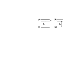
Figure 3: For the QND interaction, the levels $|1\rangle$ and $|2\rangle$ are coupled off-resonantly to states $|3\rangle$ and $|4\rangle$.

For the light, an effective spin vector can be defined, the so-called Stokes vector. Its components are given by

$$\hat{S}_{z} = \frac{1}{2}\left(\hat{a}_{1}^{\dagger}\hat{a}_{1}-\hat{a}_{2}^{\dagger}\hat{a}_{2}\right),\ \hat{S}_{x}=\frac{1}{2}\left(\hat{a}_{1}^{\dagger}\hat{a}_{2}+\hat{a}_{2}^{\dagger}\hat{a}_{1}\right),$$ (11)

$$\hat{S}_{y} = \frac{1}{2i}\left(\hat{a}_{1}^{\dagger}\hat{a}_{2}-\hat{a}_{2}^{\dagger}\hat{a}_{1}\right),$$ (12)

where $\hat{a}_{1}^{\dagger}$ and $\hat{a}_{2}^{\dagger}$ create a photon in mode $a_{1}$ and $a_{2}$, respectively. $\hat{S}_{z}$ measures the difference of photons in the two modes. By an appropriate choice of the parameters, the Hamiltonian describing the interaction of the light with the first atomic ensemble can be brought to the form QND

$$\hat{H}=\hbar\Omega_{J}\hat{S}_{z}\hat{J}_{z},$$ (13)

with a frequency $\Omega_{J}$. Due to the interaction, the collective spin vector of the atoms is rotated around the $z$ axis by $\chi_{J}\hat{S}_{z}$, with the atom–photon coupling $\chi_{J}=\Omega_{J}t$ and the effective interaction time $t$. The Stokes vector undergoes the same variation with $\chi_{J}\hat{S}_{z}$ replaced by $\chi_{J}\hat{J}_{z}$. This rotation of the Stokes vector is due to the Faraday effect of the light passing the atoms, while the rotation of the atomic spin vector is due to an AC Stark shift originating from the light field. The coupling $\chi_{J}$ is given by QND

$$\chi_{J}=2g^{2}\frac{L}{c}\frac{\Delta}{\frac{1}{4}\Gamma^{2}+\Delta^{2}},\quad g=\sqrt{\frac{\omega d^{2}}{2\hbar\epsilon_{0}AL}},$$ (14)

where $A$ and $L$ are cross section and length of the atomic sample, $\Gamma$ and $d$ are line-width and dipole moment of the atomic transition, respectively, and $\Delta$ is the detuning from the atomic resonance frequency $\omega$.

After the interaction,

$$\hat{S}_{y}^{\rm out}=\sin(\chi_{J}\hat{J}_{z})\hat{S}_{x}^{\rm in}+\cos(\chi_{J}\hat{J}_{z})\hat{S}_{y}^{\rm in},$$ (15)

and if initially

$${\langle\hat{\bf S}^{\rm in}\rangle}=\frac{n_{\!J}}{2}\hat{\bf x},\quad(\Delta\hat{S}_{x}^{\rm in})^{2}=0,\quad(\Delta\hat{S}_{y,z}^{\rm in})^{2}=\frac{n_{\!J}}{4},$$ (16)

where $n_{\!J}$ is the number of photons in the ensemble $\hat{{\bf J}}$, then we can effectively replace $\hat{S}_{x}^{\;\rm in}$ by its macroscopic expectation value $n_{\!J}/2$. Furthermore, developing the trigonometric expressions and assuming that $N_{J}\chi_{J}^{2}\ll 1$, we obtain in leading order

$$\hat{S}_{y}^{\rm out}\approx\frac{n_{\!J}\chi}{2}\hat{J}_{z}^{\rm in}+\hat{S}_{y}^{\rm in}.$$ (17)

Hence a measurement of the $y$ component of the outgoing light vector gives information about ${\langle\hat{J}_{z}\rangle}$, while $\hat{J}_{z}$ itself is not affected by the rotation around the $z$ axis.

If such a QND measurement is performed after the first beam splitter of the interferometer, then the operator

$$\hat{J}^{\prime}_{z}\equiv\hat{J}_{z}^{\rm out}-\frac{2}{n_{\!J}\chi_{J}}\hat{S}_{y}^{\rm out}$$ (18)

measures the difference between the $z$ component of the ensemble’s atomic spin vector after the second beam splitter and the estimated value after the first one. The fluctuations of this operator are reduced as compared to $\hat{J}_{z}^{\rm out}$ QND , while the fluctuations of $\hat{J}_{y}$ are enlarged, which is depicted in Fig. 4. Hence, the state of the atomic spin vector is squeezed in the $z$ direction.

III.2 III.B. Modified interferometric scheme

We modify the scheme introduced in Section II by inserting the QND interaction shortly after the first beam splitter, followed by an extra rotation around $x$ by $\pi/2$, which rotates the uncertainty ellipse such that the phase uncertainty is reduced as desired, cf. Fig. 4. In the experiment, the latter pulse must not transfer momentum to the particles, which can be achieved by using co-propagating Raman lasers for this step, provided that the two transition frequencies are approximately equal, so that the two recoil momenta cancel in the transitions.

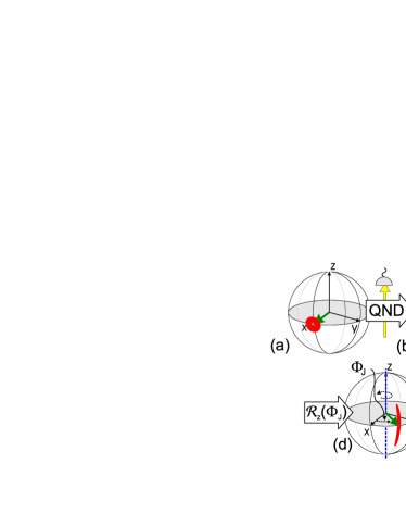
Figure 4: (Color online) The interferometric scheme for squeezed input states: (a) collective spin after the first beam splitter, (b) the QND measurement prepares a spin squeezed state which (c) is rotated around $x$ by $\pi/2$; step (d)$\to$(e) as step (b)$\to$(c) in Fig. 2.

The outgoing spin vector now is calculated as $\hat{\bf J}^{\rm out}={\cal R}_{x}(-\pi/2){\cal R}_{z}(\Phi_{J}){\cal R}_{x}(\pi/2){\cal R}_{z}(\chi\hat{S}_{z})\hat{\bf J}^{\rm in}$, and in analogy for the second ensemble $\hat{\bf L}$, with corresponding Stokes vector $\hat{\bf T}$.

In comparison to Eq. (5), $\hat{J}_{z}^{\rm out}$ now has to be corrected to incorporate the spin squeezing (ss) as described above:

$$\hat{\phi}_{\rm ss} = -\frac{1}{N_{J}}\Big{(}\hat{J}_{z}^{\rm out}-\frac{2}{n_{\!J}\chi_{J}}\hat{S}_{y}^{\rm out}\Big{)}$$ (19)

$$+\frac{1}{N_{L}}\Big{(}\hat{L}_{z}^{\rm out}-\frac{2}{n_{\!L}\chi_{L}}\hat{T}_{y}^{\rm out}\Big{)}.$$

Calculating the expectation value and variance as before yields

$${\langle\hat{\phi}_{\rm ss}\rangle} = \phi-\alpha\Big{(}\frac{1}{N_{J}}+\frac{1}{N_{L}}\Big{)}$$ (20)

$$(\Delta\hat{\phi}_{\rm ss})^{2} = \frac{1}{n\chi^{2}}\Big{(}\frac{1}{N_{J}^{2}}+\frac{1}{N_{L}^{2}}\Big{)}+\alpha\Big{(}\frac{1}{N_{J}}+\frac{1}{N_{L}}\Big{)}.$$ (21)

Here it has been assumed $n_{J}=n_{L}=:n$ and $\chi_{J}=\chi_{L}=:\chi$. Deviations from these assumptions enter the variance only in higher order terms as long as $||\chi_{J}|-|\chi_{L}||/(|\chi_{J}|+|\chi_{L}|)\ll 1$, and similar for $n_{J}$. Further assumptions leading to these expressions are $\bar{N}\chi^{2}\ll 1$ as mentioned before, as well as $n\chi^{2}\ll\sqrt{8}\cdot[\sqrt{\bar{N}}(\theta^{2}+\phi^{2})]^{-1}$. Now, provided that $\alpha$ is small enough, the variance is dominated by the first two terms scaling as $N_{J/L}^{-2}$. They originate from the projection noise of the light, and in principle allow to improve the resolution below the standard quantum limit. However, $n\chi^{2}$ equals, except for a factor of order unity, the fraction of atoms which are lost due to spontaneous processes during the squeezing process, cf. Section V. Thus, $n\chi^{2}\ll 1$ is necessary, and even though we obtained a Heisenberg-like scaling $(\Delta\hat{\phi}_{\rm ss})^{2}\sim 1/N_{J,L}^{2}$, we are far from reaching the Heisenberg limit.

Furthermore, as it becomes clear from the second term, the resolution is limited by the accuracy of the fluorescence number measurements. These measurements are necessary in any case to determine the phase, because ${\langle\hat{J}_{z}^{\rm out}\rangle}$ and ${\langle\hat{L}_{z}^{\rm out}\rangle}$ have to be rescaled properly. However, $\hat{J}_{z}$ and $\hat{L}_{z}$ itself can be measured using another QND interaction. As will be shown in the next section, this reduces the dependence on the quality of the number measurements.

III.3 III.C. QND output measurement

Let us consider now a modification of the scheme using squeezed states, where a second QND laser beam is sent through each ensemble shortly after the last beam splitter. We define

$$\hat{\phi}_{\rm ss+}=-\frac{1}{N_{J}}\frac{2}{n\chi}\Big{(}\hat{S}_{y,r}^{\rm out}-\hat{S}_{y}^{\rm out}\Big{)}$$

$$+\frac{1}{N_{L}}\frac{2}{n\chi}\Big{(}\hat{T}_{y,r}^{\rm out}-\hat{T}_{y}^{\rm out}\Big{)},$$ (22)

where the extra index $+$ is supposed to indicate the additional QND measurement. Furthermore, $\hat{{\bf S}}_{r}$ and $\hat{{\bf T}}_{r}$ correspond to individually prepared light pulses used to read out $\hat{J}_{z}$ and $\hat{L}_{z}$, respectively. The resulting expectation value and variance in leading order are

$${\langle\hat{\phi}_{\rm ss+}\rangle} = \phi+\alpha\theta\Big{(}\frac{1}{N_{J}}+\frac{1}{N_{L}}\Big{)}$$ (23)

$$(\Delta\hat{\phi}_{\rm ss+})^{2} = \frac{2}{n\chi^{2}}\Big{(}\frac{1}{N_{J}^{2}}+\frac{1}{N_{L}^{2}}\Big{)}$$ (24)

$$+\alpha(\theta^{2}+\phi^{2})\Big{(}\frac{1}{4N_{J}}+\frac{1}{4N_{L}}\Big{)}.$$

Let us compare the modified scheme including an additional QND measurement with the scheme using squeezed states. The magnitude of $\alpha$ in the variance of the modified scheme is effectively reduced for small $\theta$ and $\phi$, $\alpha\to\alpha(\theta^{2}+\phi^{2})/4$, as compared to Eq. (21). Hence, the dependence on the number measurement is reduced. Furthermore, the leading term shifting the expectation value from the desired result $\phi$ is smaller by a factor $\theta$ as compared to Eq. (20).

As a further possible advantage, the effect of a non-symmetric atom-light interaction is compensated if the coupling of the read-out QND pulse is similar to the coupling of the squeezing pulse kuzmichPRL . However, this advantage is probably not very relevant for the Sagnac interferometer considered here due to the long time-of-flight of the ensembles in the interferometer between the two QND pulses.

A disadvantage of this scheme is that the first term of the variance of Eq. (24) comes with a factor of $2$ because of the two projection measurements of the light necessary per atomic ensemble. It is possible, although technically demanding, to reduce this contribution by re-using the light from the first QND interaction for the read-out. In this case, $\chi\to-\chi$ is needed in the second interaction in order to obtain the difference $\hat{J}_{z}^{\rm out}-\hat{J}_{z}^{\rm in}$ kuzmichPRL , and in analogy for the second ensemble. The sign can also be achieved by a $\pi$ rotation of the atom spin vector around the $x$ axis in between the final beam splitter and the QND read-out pulse.

IV IV. Jointly squeezed ensembles

In the preceding section we have seen that the $1/(n\chi^{2}N_{J}^{2})$ term in the variance comes with a factor given by the number of QND interactions with different ensembles of light, cf. Eq. (24). For this reason let us consider the case of preparing the initial state of the two atomic ensembles with only a single QND pulse that interacts with both ensembles consecutively. The first interaction (with ensemble $\hat{{\bf J}}$) transforms $\hat{{\bf J}}^{\text{in}}\rightarrow{\cal R}_{z}(\chi\hat{S}_{z}^{\rm in})\hat{{\bf J}}^{\text{in}}$, the second interaction (with ensemble $\hat{{\bf L}}$) transforms $\hat{{\bf L}}^{\text{in}}\rightarrow{\cal R}_{z}(\chi\hat{S}_{z}^{\rm in})\hat{{\bf L}}^{\text{in}}$, because $\hat{S}_{z}^{\rm in}$ itself remains unchanged during the QND interaction. The Stokes vector $\hat{{\bf S}}$ transforms as $\hat{{\bf S}}^{\text{out}}={\cal R}_{z}(\chi\hat{L}_{z}^{\rm in}){\cal R}_{z}(\chi\hat{J}_{z}^{\rm in})\hat{{\bf S}}^{\text{in}}$, and the $y$ component of the outgoing light is given by

$$\hat{S}_{y}^{\text{out}} = \cos(\chi\hat{L}_{z}^{\rm in})\left[\cos(\chi\hat{J}_{z}^{\,\rm in})\hat{S}_{y}^{\,\rm in}+\sin(\chi\hat{J}_{z}^{\,\rm in})\hat{S}_{x}^{\,\rm in}\right]+$$ (25)

$$\,\sin(\chi\hat{L}_{z}^{\rm in})\left[\cos(\chi\hat{J}_{z}^{\,\rm in})\hat{S}_{x}^{\,\rm in}-\sin(\hat{J}_{z}^{\,\rm in}\chi)\hat{S}_{y}^{\,\rm in}\right],$$

such that for $N\chi^{2}\ll 1$, and $\hat{{\bf S}}$ initially prepared as in Eq. (16), we have

$$\hat{S}_{y}^{\text{out}}\approx\frac{n\chi}{2}(\hat{J}_{z}^{\,\rm in}+\hat{L}_{z}^{\rm in})+\hat{S}_{y}^{\,\rm in}.$$ (26)

Measuring $\hat{S}_{y}^{\text{out}}$ thus reveals information about $\hat{J}_{z}^{\rm in}+\hat{L}_{z}^{\rm in}$ and performs a squeezing operation on this joint operator. Now we apply the same operations as before to the ensemble $\hat{{\bf J}}$, but for the ensemble $\hat{{\bf L}}$ we perform a rotation by $\pi$ around the $x$ axis before the final measurement. After the extra pulse, the Sagnac shift $\phi$ is effectively encoded in the sum of the $z$ components instead of into the difference.

We define the phase operator for the scheme employing jointly squeezed (js) ensembles as

$$\hat{\phi}_{\rm js}=-\Big{(}\frac{1}{N_{J}}\hat{J}_{z}^{\,\text{out}}+\frac{1}{N_{L}}\hat{L}_{z}^{\text{out}}-\frac{2}{n\chi\bar{N}}\hat{S}_{y}^{\,\text{out}}\Big{)}.$$ (27)

Note that in this definition $\hat{J}_{z}^{\,\text{out}}$ and $\hat{L}_{z}^{\text{out}}$ are divided by the atom numbers of the respective ensembles as before, while the QND measurement yields an estimate of $\hat{J}_{z}^{\,\text{out}}+\hat{L}_{z}^{\text{out}}$ without such a correction, cf. Eq. (26). As a consequence we expect that we loose the advantages of squeezing if the numbers of atoms in the two ensembles differ strongly, i.e., if $\gamma\gg 1$. We find in leading order

$${\langle\hat{\phi}_{\rm js}\rangle} = \phi-\frac{2\alpha}{\bar{N}}$$ (28)

$$(\Delta\hat{\phi}_{\rm js})^{2} = \frac{1}{n\chi^{2}\bar{N}^{2}}+\frac{2\alpha}{\bar{N}}+\frac{\gamma^{2}}{8\bar{N}^{2}}.$$ (29)

The importance of the number fluctuations at the preparation stage is reflected in the fact that in order to arrive at these equations, the assumption

$$\gamma\sqrt{\bar{N}}(n\chi^{2})^{2}(\theta^{2}+\phi^{2})\ll 1$$ (30)

is necessary in addition to the assumptions leading to Eq. (21). Furthermore, now $1/(n\chi^{2}\bar{N}^{2})$ is the leading term only if $n\chi^{2}\gamma^{2}/8\ll 1$.

A QND measurement could also be used after the interferometer to directly read out the joint observable $\hat{J}^{\text{out}}_{z}+\hat{L}_{z}^{\text{out}}$ by defining

$$\hat{\phi}_{\rm js+}=-\frac{2}{n\chi}\frac{1}{\bar{N}}\left(\hat{S}_{y,r}^{\text{out}}-\hat{S}_{y}^{\text{out}}\right),$$ (31)

where again the indices $r$ refers to the read-out QND measurement. Notice that in this way it is not possible to measure the correct rescaled observable $\hat{J}_{z}^{\text{out}}/N_{J}+\hat{L}_{z}^{\text{out}}/N_{L}$, and consequently there is an important contribution from the difference of the atom numbers in the expectation value already:

$${\langle\hat{\phi}_{\rm js+}\rangle}=\phi+\frac{N_{L}-N_{J}}{N_{L}+N_{J}}\theta+\frac{\alpha\phi}{2\bar{N}}.$$ (32)

Compared to the variance of the scheme using jointly squeezed ensembles without the QND read-out measurement, Eq. (29), the dependence of the variance on the number measurements and on the atom number difference in the two ensembles is reduced for small $\theta,\,\phi$:

$$(\Delta\hat{\phi}_{\rm js+})^{2} = \frac{2}{n\chi^{2}\bar{N}^{2}}+\frac{\alpha}{2\bar{N}}(\theta^{2}+\phi^{2})+$$ (33)

$$\,\,+\frac{\gamma^{2}}{8\bar{N}^{2}}\alpha(\theta^{2}+\phi^{2}).$$

However, the $\gamma$-dependent correction to the expectation value ${\langle\hat{\phi}_{\rm js+}\rangle}$ is only negligible compared to the standard deviation $\Delta\phi_{\rm js+}$ if $\gamma^{2}\bar{N}n\chi^{2}\theta^{2}/8\ll 1$. This is generally a stronger criterion than the limit on $\gamma$ encountered without the QND read-out, cf.Eq. (30).

The offset can be compensated by using an estimate for $\theta$ from the final fluorescence measurement

$$\hat{\theta}=-\frac{1}{N_{J}}\hat{J}_{z}^{\text{out}}+\frac{1}{N_{L}}\hat{L}_{z}^{\text{out}},$$ (34)

to define a corrected phase operator

$$\hat{\phi}^{c}_{js+}=\hat{\phi}_{js+}-\frac{N_{L}-N_{J}}{N_{L}+N_{J}}\hat{\theta}$$ (35)

which takes into account the bias of ${\langle\hat{\phi}_{\rm js+}\rangle}.$ We find that to leading order

$${\langle\hat{\phi}^{c}_{\rm js+}\rangle} = \phi+\frac{\alpha\phi}{2\bar{N}}-\frac{\gamma^{2}\alpha}{2\bar{N}^{2}}$$ (36)

$$\left(\Delta\hat{\phi}^{c}_{\rm js+}\right)^{2} = \frac{2}{n\chi^{2}\bar{N}^{2}}+\frac{\alpha\phi^{2}}{2\bar{N}}+\frac{\gamma^{2}}{8\bar{N}^{2}}.$$ (37)

Hence, the $\gamma$-dependent bias in the expectation value is reduced by a factor $\alpha\gamma/(\bar{N}^{3/2}\theta)\ll 1$, while the $1/\bar{N}$ term in the variance still has a factor $\alpha\phi^{2}$.

These are the same advantages that we also found in the case of separately squeezed ensembles with QND read-out, cf. Eq. (24). However, the contribution of the term proportional to $1/n\chi^{2}\bar{N}^{2}$ is reduced by a factor of $2$ in $(\Delta\hat{\phi}^{c}_{\rm js+})^{2}$, because only two instead of four projective measurements of the light are necessary in this case.

V V. Decoherence

The attainable squeezing is limited by the absorption of photons during the interaction between light and atoms squeezingGaussian . Each atom which absorbs and subsequently spontaneously emits a photon is no longer correlated to the rest of the atoms, but still adds to the variance. We estimate the number of atoms contributing to such an uncorrelated background as the number of scattered photons $n\kappa$, where $\kappa=N_{J}\chi\Gamma/\Delta$ is the optical density. Then, in the limit of $\kappa\ll 1$ and for just a single ensemble, one finds squeezingGaussian

$${\langle J_{z}^{\,\rm out}\rangle} \rightarrow {\langle J_{z}^{\,\rm out}\rangle}\left(1-\frac{n\chi\Gamma}{\Delta}\right),$$ (38)

$${\langle\left(J_{z}^{\,\rm out}\right)^{2}\rangle} \rightarrow \left(1-\frac{n\chi\Gamma}{\Delta}\right)^{2}{\langle\left(J_{z}^{\,\rm out}\right)^{2}\rangle}+\frac{nN_{J}\chi\Gamma}{2\Delta}$$ (39)

for the collective atomic spin vector and

$${\langle S_{z}^{\,\rm out}\rangle} \rightarrow {\langle S_{z}^{\,\rm out}\rangle}\left(1-\frac{N_{J}\chi\Gamma}{\Delta}\right),$$ (40)

$${\langle\left(S_{z}^{\,\rm out}\right)^{2}\rangle} \rightarrow \left(1-\frac{N_{J}\chi\Gamma}{\Delta}\right)^{2}{\langle\left(S_{z}^{\,\rm out}\right)^{2}\rangle}+\frac{N_{J}^{2}\chi\Gamma}{4\Delta}$$ (41)

for the Stokes vector. The leading order corrections to the variance $(\Delta\hat{\phi}_{\rm ss})^{2}$ given in Eq. (21) for the case of separately squeezed ensembles reads

$$(\Delta\hat{\phi}_{\rm ss})^{2} \rightarrow (\Delta\hat{\phi}_{\rm ss})^{2}+\frac{n\chi\Gamma}{\Delta}\frac{1}{\bar{N}}+\frac{2\Gamma}{n^{2}\chi\Delta},$$ (42)

and similarly for the other schemes. We will use this estimate in the following discussion and leave an in-depth analysis of decoherence processes, e.g., following the lines of squeezingGaussian , to further investigations. Generally, according to Eq. (38) also the expectation value changes due to decoherence. This can be accounted for by rescaling, and doing so gives only higher-order corrections to Eq. (42).

For usual choices of parameters, the last term in Eq. (42) is negligible, while the contribution proportional to $\bar{N}^{-1}$ is comparable in size to the terms in Eq. (21). This limits the coupling $\chi$ and thus the achievable squeezing. For all other experimental parameters fixed, there exists an optimal choice for the detuning $\Delta$ and thus for $\chi$ [see Eq. (14)] which minimizes the variance. Taking into account only the first term in Eq. (21), and in the limit $\Delta\gg\Gamma$, this optimal choice of $\Delta$ leads to a minimal value for $(\Delta\hat{\phi}_{\rm ss})^{2}$:

$$\min_{\Delta}\left[(\Delta\phi_{\rm ss})^{2}\right]=\frac{2}{N^{\frac{3}{2}}\,d}\sqrt{\frac{2\epsilon_{0}\hbar cA\Gamma}{\omega}}.$$ (43)

The scaling is thus no longer as in the Heisenberg limit, but it is still better than in shot-noise limited measurements (see also auzinsh:2004 ).

In addition, the decay of the states $|1\rangle$ and $|2\rangle$ during the interferometer step has to be taken into account. Choosing long-lived hyperfine ground-state levels to implement $|1\rangle$ and $|2\rangle$ minimizes this decay. Also, spin squeezed states have been shown to be robust with respect to both, particle loss and dephasing stockton:2003 , in contrast to, e.g., GHZ states, which are maximally fragile under particle losses.

VI VI. Comparison of the schemes

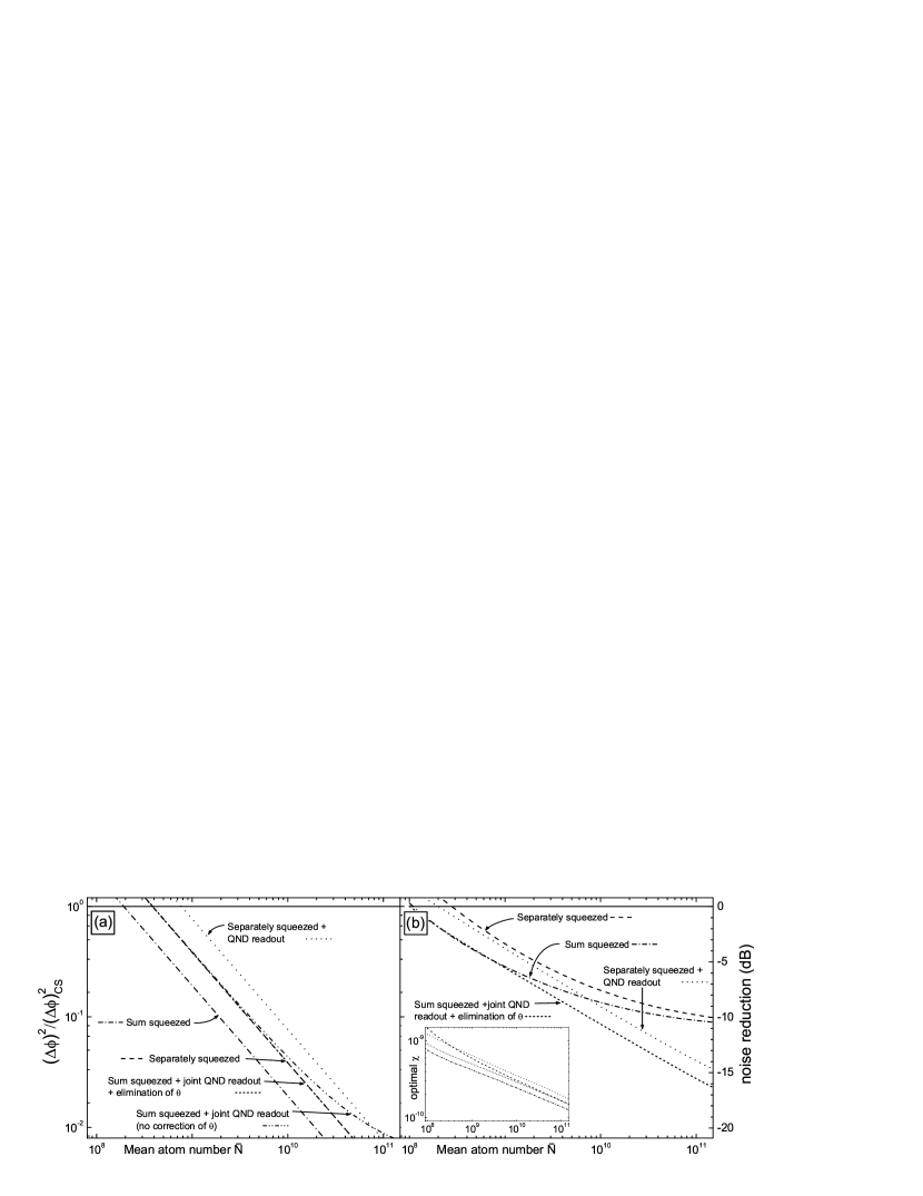
Figure 5: Double-logarithmic plot of the variances $(\Delta\phi)^{2}$ for the methods discussed in the text normalized to the variance for coherent states $(\Delta\phi_{\rm cs})^{2}$, as a function of the mean number of atoms $\bar{N}$. The scale on the right hand site gives the noise reduction in dB. In both figures $n=10^{11}$, and we fixed $\theta=\phi=0.01$ in order to operate close to the point of maximal sensitivity of the interferometer. In (a) we consider the close-to-ideal scenario with $\alpha=2\times 10^{-7}$, $\gamma=10$, and decoherence is not included. $\chi=3.23\times 10^{-10}$ is used, corresponding to a detuning $\Delta=2.28\times 10^{10}\;$s^-1 for the Rb D₂ line and a cross section $A=0.3\;$mm² of the laser beam. In this close-to-ideal scenario, the scaling as $\bar{N}^{-2}$ is visible for all the methods employing squeezing. The graphs for separately squeezed ensembles (without QND read-out) and for jointly squeezed ensembles with QND read-out and corrected expectation value lie on top of each other. In the case of a joint QND read-out, failing to correct the expectation value for the contribution from $\theta$ results in a scaling as $1/\bar{N}$ for $\bar{N}\gtrsim 10^{9}$. (b) Realistic scenario with $\alpha=2\times 10^{-2}$, $\gamma=10^{4}$, and including decoherence. In each case and for each value of $\bar{N}$ the detuning has been adjusted to minimize the variance parameters . The inset shows the corresponding optimal values of the coupling parameter $\chi$. For large atom numbers it is clearly seen that the schemes which do not employ a final QND measurement are strongly affected by the limitations from the fluorescence detection. The curve for jointly squeezed ensembles using a joint QND readout lies outside the range of the figure.

To analyze the performance of the schemes discussed in the preceding sections we will fix the number of photons as $n=10^{11}$ and take $\bar{N}=10^{10}$ as a reasonable parameter for the mean atom number per ensemble. We will first consider a close-to-ideal scenario and assume that the noise from the fluorescence measurements can be neglected by setting $\alpha=2\times 10^{-7}$. Also, we will set $\gamma=10$, which for $\bar{N}=10^{10}$ atoms corresponds to $|N_{J}-N_{L}|=10^{-4}\bar{N}$, and we will initially not include decoherence. Fig. 5 (a) shows the scaling with $\bar{N}$ of $(\Delta\phi)^{2}/(\Delta\phi_{\rm cs})^{2}$, i.e., of the various variances normalized to the case of coherent ensembles. For all the methods involving squeezing of some observable a Heisenberg like scaling is visible. The offsets of these curves are given by the numbers of QND measurements performed, i.e., by the factor multiplying the $1/(n\chi^{2}\bar{N}^{2})$ term in the variance of each of the considered schemes that involve squeezing. For the measurement of $\phi$ via reading out $\hat{J}_{z}+\hat{L}_{z}$ through a QND interaction, the term proportional to $\theta$ shifting the expectation value [see Eq. (32)] has been included into the variance, in order to allow for a fair comparison. It is this term which makes the variance scale only proportional to $1/\bar{N}$ for $\bar{N}\gtrsim 10^{9}$. Obviously, correcting this contribution of $\theta$ as described in Section IV avoids this term and maintains the improvement by a factor of $2$ compared to the case of squeezing and QND measuring both ensembles separately.

In Fig. 5 (b), the relative variances are plotted for realistic experimental parameters and including decoherence. $\alpha=2\times 10^{-2}$ corresponds to $50$ fluorescence cycles per atom, and $\gamma=10^{4}$ is equivalent to a difference of the number of atoms in the two ensembles of $10$% of the mean number $\bar{N}$ at $\bar{N}=10^{10}$. With all other parameters fixed, for each value of $\bar{N}$ the interaction strength $\chi$ is determined by choosing the detuning $\Delta$ from atomic resonance such that the variance $(\Delta\phi)^{2}$ is minimized, see Eq. (43) parameters .

As can be seen from Fig. 5 (b), in such a realistic scenario the noise reduction obtained from squeezing decreases for all methods. For large atom numbers, in all cases the variance scales as $1/\bar{N}$ due to decoherence and the noise from the fluorescence measurements. For all the procedures not involving a QND read-out, the strong influence of the latter contribution can be observed, though for $\bar{N}=10^{10}$ atoms the total noise still is reduced by around $7\;$dB with respect to the limit set by quantum projection noise. On the other hand, the read-out via QND measurements allows to reduce the noise by more than $10\;$dB compared to this limit, while this method does not require an additional experimental setup as compared to the scheme where QND measurements are performed only on the incoming atomic ensembles.

While in the close-to-ideal case squeezing of a joint observable gives an advantage of a factor of $2$ in the variance compared to individual squeezing and read-out (corresponding to a $3\;$dB noise reduction), for an experimental reasonable scenario this advantage reduces to about $1.5\;$dB. Of course the method of squeezing a joint observable of both ensembles has a basic advantage since it only needs a single squeezing operation instead of two, and thus less technical effort is necessary.

VII VII. Entangled ensembles

Julsgaard et al. demonstrated experimentally in Ref. Polzik the generation of macroscopic entanglement between two atomic ensembles. The scheme to generate such a macroscopically entangled state, described first in Ref. Duan1 , is motivated by the fact that under the ideal condition of $\gamma=0$ two commuting joint observables can be constructed from $\hat{{\bf J}}$ and $\hat{{\bf L}}$:

$${\langle[\hat{J}_{y}-\hat{L}_{y},\hat{J}_{z}+\hat{L}_{z}]\rangle}\propto(N_{J}-N_{L})=0,$$ (44)

i.e., $\hat{J}_{y}-\hat{L}_{y}$ can be measured without affecting $\hat{J}_{z}+\hat{L}_{z}$, and vice versa. This can be seen directly from

$$({\cal R}_{z}(\chi\hat{S}_{z})\hat{{\bf J}}^{\text{in}}-{\cal R}_{z}(\chi\hat{S}_{z})\hat{{\bf L}}^{\text{in}})_{y}=\hat{J}_{y}^{\text{in}}-\hat{L}_{y}^{\text{in}},$$ (45)

i.e., the first QND interaction leaves the difference of the $y$ components unaffected. Thus after squeezing the sum $\hat{J}_{z}+\hat{L}_{z}$, also the difference $\hat{J}_{y}-\hat{L}_{y}$ can be squeezed without loosing the information gained in the first measurement. To realize this experimentally in the interferometer, after the first squeezing interaction $\hat{\bf J}$ is rotated by a classical $\pi/2$ pulse around the $x$ axis so that $\hat{J}_{y}\to\hat{J}_{z}$ while $\hat{\bf L}$ is rotated by $-\pi/2$ around $x$ giving $-\hat{L}_{y}\to\hat{L}_{z}$. Then a second laser pulse, prepared again as in Eq. (16), interacts consecutively with both ensembles and thus finally carries information about $\hat{J}_{y}-\hat{L}_{y}$. The outgoing state corresponds to a macroscopically entangled EPR state Duan1 . It is now a natural question to ask whether entangled atomic ensembles are of use in Sagnac atom interferometry.

For the schemes discussed so far, the collective spin vectors lie in the $x-z$ plane after the last step of the interferometer. Therefore always ${\langle\hat{J}_{y}-\hat{L}_{y}\rangle}=0$, and an additional operation is necessary in order to encode phase information in the $y$ components as well. This can be achieved by rotating both ensemble vectors $\hat{{\bf J}}$ and $\hat{{\bf L}}$ by an angle $\varphi$ and $-\varphi$ around the $x$ axis before and after the interferometric phase is applied, respectively. In this way the plane of rotation of the phase shift is effectively tilted by $\varphi$ around the $x$ axis.

The measurement process now consists of first rotating $\hat{{\bf J}}$ and $\hat{{\bf L}}$ by $\pm\pi/2$ and using another QND interaction to measure the sum of the $z$ components. This measurement, scaled correctly by a $\varphi$-dependent factor, reveals $\phi$. To be more explicit, the corresponding operator for entangled ensembles (EE) reads

$$\hat{\phi}_{\rm EE}=\frac{1}{\cos\varphi}\frac{2}{\bar{N}n\chi^{2}}\left(\hat{S}^{\rm out}_{y,r}-\hat{S}^{\rm out}_{y}\right).$$ (46)

A measurement of the sum of the $y$ components can be realized after another rotation around $x$ by either a QND or a projection measurement. In the former case

$$\hat{\theta}_{\rm EE}=\frac{1}{\sin\varphi}\frac{2}{\bar{N}n\chi^{2}}\left(\hat{T}_{y,r}^{\rm out}-\hat{T}^{\rm out}_{y}\right).$$ (47)

These measurements yield both angles:

$${\langle\hat{\phi}_{\rm EE}\rangle} = \phi+\frac{N_{L}-N_{J}}{N_{L}+N_{J}}\theta+\frac{\alpha\;\phi}{2\bar{N}}$$ (48)

$${\langle\hat{\theta}_{\rm EE}\rangle} = \theta+\frac{N_{L}-N_{J}}{N_{L}+N_{J}}\phi+\frac{\alpha\;\theta}{2\bar{N}},$$ (49)

where the offsets can be corrected as above. For parameters as in Section V. the leading terms of the corresponding variances read (at $\theta=0$ and $\phi=0$)

$$(\Delta\hat{\phi}_{\rm EE})^{2} = \frac{1}{\cos^{2}\varphi}\frac{2}{\bar{N}^{2}n\chi^{2}}+\frac{\gamma^{2}\;n\chi^{2}}{8\bar{N}}.$$ (50)

$$(\Delta\hat{\theta}_{\rm EE})^{2} = \frac{1}{\sin^{2}\varphi}\frac{2}{\bar{N}^{2}n\chi^{2}}+\frac{\gamma^{2}\;n\chi^{2}}{8\bar{N}}.$$ (51)

Changing $\varphi$ allows to trade in a lower variance of one component for a higher variance of the other. But these variances are only scaling with $1/\bar{N}^{2}$ if $\gamma$ is close to zero, otherwise the last term $\propto\gamma^{2}n\chi^{2}/\bar{N}$ in Eqs. (50) and (51) is dominating the scaling. However, $\gamma\approx 0$ is an obvious requirement in this case, as otherwise the commutator does not vanish in Eq. (44), and thus the two squeezing operations are not compatible.

VIII VIII. Conclusion and outlook

We have presented and compared in detail several methods to improve the detection of a differential phase shift of two atomic interferometers beyond the standard quantum limit, having in mind especially the application to Sagnac interferometry. For this purpose, we have analyzed the squeezing of individual and joint observables and, in both cases, the read-out of the interferometer via fluorescence detection of the atoms only or by an additional QND interaction.

If decoherence and measurement imperfections are neglected, all the methods of squeezing improve the behavior of the variance of the differential phase to a $1/\bar{N}^{2}$ scaling, modified by a factor $k/(n\chi^{2})\gg 1$, which is determined by the number $k$ of QND interactions involved, by the number of photons $n$, and by the coupling $\chi$ between atoms and photons. In the case of jointly squeezed observables, we found that this limit can only be attained if some constraints on the difference of the number of atoms in both ensembles can be fulfilled. In all cases, the achievable squeezing is limited by decoherence due to the absorption of photons during the QND measurement.

Using fluorescence measurements to read out the atomic spins after the interferometer always produces additional noise scaling as $1/\bar{N}$ due to the photon shot noise. As an alternative method, a QND measurement can be employed to read out the final state of the interferometer. Although in this case fluorescence measurements are still necessary to determine the number of atoms in the two ensembles, their contribution to the noise is reduced to a large extent. We have shown that the best method to achieve this is to perform squeezing and read-out via a QND measurement of a joint observable of the two ensembles, provided that the difference between the number of atoms in the two ensembles can be made smaller than approximately $10$% of the mean number of atoms. This procedure minimizes the number of QND interactions necessary, thereby minimizing the factor multiplying the $1/\bar{N}^{2}$ term in the variance, and it reduces the experimental effort.

Finally, we considered the creation of a macroscopically entangled state of the two atomic ensembles via squeezing of two non-local, commuting observables. We showed that in this case both the sum and the difference of the phase shifts can be measured with a variance scaling with $1/\bar{N}^{2}$, and that the relative uncertainty can be shifted between both quantities. However, this scaling can only be reached here if the number difference between the two ensembles can be made very small. Therefore, it would be desirable to identify methods to control the numbers of atoms in the ensembles, for instance by employing the superfluid – Mott insulator transition in an optical lattice embedded in a weakly confining harmonic potential micirac ; mibloch . Controlling this confinement, which plays the role of a local chemical potential, the number of atoms in the Mott phase at $T>0$ can be controlled and should only depend mildly on the total number of atoms in the system. A detailed analysis of this idea is left for future investigations.

IX VIII. Acknowledgments

It is a pleasure to thank H.A. Bachor, M. Drewsen, J. Eschner, P. Grangier, O. Gühne, K. Mølmer, and A. Sanpera for illuminating discussions. This work has been supported by the DFG (SPP 1116, SPP 1078, GRK 282, POL 436, CRK, and SFB 407), by the EC (QUPRODIS, FINAQS), and by the ESF (QUDEDIS). UVP acknowledges support from the Danish Natural Science Research Council.

References

- (1) R. Bluhm, V.A. Kostelecky, C.D. Lane, and N. Russell, Phys. Rev. Lett. 88, 090801 (2002).
- (2) C. Jentsch, T. Müller, E. Rasel, and W. Ertmer, Gen. Rel. Grav. 36, 2197 (2004).
- (3) S. Fray, C. Alvarez-Diez, T.W. Hänsch, and M. Weitz, Phys. Rev. Lett. 93, 240404 (2004).
- (4) M.J. Snadden, J.M. McGuirk, P. Bouyer, K.G. Haritos, and M.A. Kasevich, Phys. Rev. Lett. 81, 971 (1998).
- (5) J.M. McGuirk, G.T. Foster, J.B. Fixler, M.J. Snadden, and M.A. Kasevich, Phys. Rev. A 65, 033608 (2002).
- (6) M.A. Kasevich and S. Chu, Phys. Rev. Lett. 67, 181 (1991)
- (7) A. Peters, K.Y. Chung, and S. Chu, Metrologia 38, 25 (2001).
- (8) B. Yurke, S.L. McCall, and J.R. Klauder, Phys. Rev. A 33, 4033 (1986).
- (9) P. Kok, S.L. Braunstein, and J.P. Dowling, Jour. Opt. B 6, 811 (2004).
- (10) D. Oblak, J.K. Mikkelsen, W. Tittel, A.K. Vershovski, J.L. Sørensen, P.G. Petrov, C.L. Garrido Alzar, and E.S. Polzik, preprint: quant-ph/0312165 (2003).
- (11) A. Kuzmich, N.P. Bigelow, and L. Mandel, Europhys. Lett. 42, 481 (1998).
- (12) A. Kuzmich, K. Mølmer, and E.S. Polzik, Phys. Rev. Lett. 79, 4782 (1997); J. Hald, J.L. Sørensen, C. Schori, and E.S. Polzik, Phys. Rev. Lett. 83, 1319 (1999).
- (13) C. Mewes and M. Fleischhauer, Phys. Rev. A 66, 033820 (2002); H. Kaatuzian, A. Rostami, A.A. Oskouei, preprint: quant-ph/0402057 (2004); D.N. Matsukevich and A. Kuzmich, Science 306, 663 (2004); B. Julsgaard, J. Sherson, J.I. Cirac, J. Fiurášek, and E.S. Polzik, Nature 432, 482 (2005).
- (14) A. S. Sørensen and K. Mølmer, Phys. Rev. Lett. 86, 4431 (2001).
- (15) L.M. Duan, J.I. Cirac, P. Zoller, and E.S. Polzik, Phys. Rev. Lett. 85, 5643 (2000).
- (16) B. Julsgaard, A. Kozhekin, and E. Polzik, Nature 413, 400 (2001).
- (17) V. Petersen, L.B. Madsen, and K. Mølmer, Phys. Rev. A 71, 012312 (2005).
- (18) T.L. Gustavson, A. Landragin, and M.A. Kasevich, Class. Quantum Grav. 17, 2385 (2000).
- (19) B. Young, M. Kasevich, and S. Chu, Precision Atom Interferometry with Light Pulses, in: Atom interferometry, ed. by P.R. Berman, Academic Press 1997.
- (20) G. Santarelli et al., Phys. Rev. Lett. 82, 4619 (1999).
- (21) A. Kuzmich and T. A. B. Kennedy, Phys. Rev. Lett. 92, 030407 (2004).
- (22) L.B. Madsen and K. Mølmer, Phys. Rev. A 70, 052324 (2005).
- (23) M. Auzinsh, D. Budker, D.F. Kimball, S.M. Rochester, J.E. Stalnaker, A.O. Sushkov, and V.V. Yashchuk, Phys. Rev. Lett. 93, 173002 (2004).
- (24) J.K. Stockton, J.M. Geremia, A.C. Doherty, H. Mabuchi, Phys. Rev. A 67, 022112 (2003).
- (25) For the parameters in the figure, the optimal values for the detuning and the interaction parameter are (at atoms for the Rb D2 line and a laser beam cross section of mm2): separately squeezed ensembles s-1, ; separately squeezed ensembles (QND readout) s-1, ; joint squeezing s-1, ; joint squeezing (QND readout and correction) s-1, .
- (26) D. Jaksch, C. Bruder, J.I. Cirac, C. W. Gardiner, and P. Zoller, Phys. Rev. Lett. 81, 3108 (1998).
- (27) M. Greiner, O. Mandel, T. Esslinger, T.W. Hänsch, and I. Bloch, Nature 415, 39 (2002).