Extended Jaynes-Cummings models and (quasi)-exact solvability

Abstract

The original Jaynes-Cummings model is described by a Hamiltonian which is hermitian and exactly solvable. Here we extend this model by several types of interactions leading to a non hermitian operator which doesn’t satisfy the physical condition of space-time reflection symmetry (PT symmetry). The new Hamiltonians are either exactly solvable admitting an entirely real spectrum or quasi exactly solvable with a real algebraic part of their spectrum.

1 Introduction

Several new theoretical aspects of quantum mechanics have been developped in the last years. In series of papers (see e.g. [1, 2] and [3] for a recent review) it is shown that the traditional self adjointness requirement of the Hamiltonian operator is not a necessary condition to guarantee a real spectrum and that the weaker condition of PT-invariance of the Hamiltonian is sufficient for that purpose. An alternative possibility for an operator to admit a real spectrum is also developed in [4]. It is the notion of pseudo-hermiticity. Following the ideas of [4], we remind here that a Hamiltonian is called $\eta$ pseudo-hermitian if it satisfies the relation $\eta H\eta^{-1}=H^{\dagger}$, where $\eta$ denotes a linear hermitian operator. It is this new notion (i.e pseudo-hermiticity property) of non hermitian Hamiltonians which explains the reality of their energy spectrum. This important property has further been considered in Refs.[5, 6].

Another direction of development of quantum mechanics is the notion of quasi exact solvability [7, 8]. It provides techniques to construct linear operators preserving a finite dimensional subspace ${\cal V}$ of the Hilbert space. Accordingly, the so called Quasi Exactly Solvable operators, once restricted on ${\cal V}$ can be diagonalized by means of algebraic methods. The QES property is strongly connected to finite dimensional representation of Lie or graded Lie algebras [7, 9, 10]. Amongst many models used to describe quantum properties of physical systems, the Jaynes-Cummings model play an important role [11, 12, 13, 14]. It describes, in a simple way the interaction of photons with a spin-1/2 particle. From the mathematical point of view, the Jaynes-Cummings model is described by a self-adjoint operator and it is completely solvable in a sense that the entire spectrum can be computed algebraically.

The purpose of this paper is to consider operators generalizing the Jaynes-Cummings Hamiltonians which are neither self-adjoint nor PT-invariant but which are pseudo-hermitian with respect to two different operators. In particular, from the original Jaynes-Cummings model (JCM in the following), we construct an extended one by adding a polynomial of the form $P(a^{\dagger},a)$ ($a^{\dagger},a$ are the usual creation and annihilation operators) of degree $d\geq 2$ in the diagonal part of the hamiltonian. Some particular choices of $P$ are constructed in such a way that the resulting operator becomes QES. The non-diagonal interaction part is also modified in such a way that (i) multiple photon exchanges are allowed and (ii) the full operator can be hermitian or pseudo-hermitian.

Here is the plan of the paper. In section 2, we revisit the Hamiltonian considered in Ref.[5] and express it in terms of differential operator of a real variable $x$. This reveals its exact solvability in terms of differential operators acting on sets of polynomials of appropriate degrees in $x$. In Sect. 3 we propose a family of operators which generalize the original JC Hamiltonian in several respects. The (pseudo)-hermiticity of these operators are analysed and the spectra and the eigenvectors are computed in details for a few of them. The differences in the spectrum corresponding to Hermitian and pseudo-Hermitian are pointed out. In particular, the energy eigenvalues are entirely real in spite of the fact that they are associated to a non hermitian and non $PT$-invariant Hamiltonian. The reality of those eigenvalues is ensured by the pseudo-hermiticity of the Hamiltonians. The section 4 is devoted to QES extensions of the JCM. These are constructed in such a way that, both, one-photon and two-photons exchange terms coexist in the non-diagonal interacting terms. By construction, these new models preserve finite dimensional vector spaces of the Hilbert spaces ,the algebraic part of the spectrum is computed in Sect 5. Further properties of these new types of QES operators, say $H_{T}$, can be discussed. Namely, following the ideas of [15] we show in Sect. 6 that the solutions of the spectral equation $H_{T}\psi=E\psi$ for generic values of $E$ lead to new types of recurence relations. The relations between $H_{T}$ and specific graded algebras are pointed out in Sect 7. Finally, the section 8 is kept for concluding remarks.

2 Exactly solvable pseudo-hermitian Hamiltonian

In this section we consider the Hamiltonian describing a system of a spin-$\frac{1}{2}$ particle in the external magnetic field, $\vec{B}$ which couples to a harmonic oscillator through some nonhermitian interaction [5]

$$H=\mu\vec{\sigma}\cdot\vec{B}+\hbar\omega a^{\dagger}a+\rho(\sigma_{+}a-\sigma_{-}a^{\dagger}).$$ (1)

Here $\vec{\sigma}$ denotes Pauli matrices, $\rho$ is some arbitrary real parameter and $\sigma_{\pm}\equiv\frac{1}{2}[\sigma_{x}\pm i\sigma_{y}]$. $\sigma_{+}$ and $\sigma_{-}$ can be expressed in matrix form

$$\sigma_{+}=\left(\matrix{0&1\cr 0&0\cr}\right)\ \ ,\ \ \sigma_{-}=\left(\matrix{0&0\cr 1&0\cr}\right).$$ (2)

Our purpose is to relate the Hamiltonian above to an appropriate differential operator preserving a family of spaces of polynomials in the variable $x$, following the ideas of exactly and quasi-exactly solvable operators [7]. With this aim, we use the usual creation and annihilation operators respectively $a^{\dagger}$ and $a$ which are defined as follows

$$a^{\dagger}=\frac{p+im\omega x}{\sqrt{2m\omega\hbar}}\ \ ,\ \ a=\frac{p-im\omega x}{\sqrt{2m\omega\hbar}},$$ (3)

where $p=-i\frac{d}{dx}$. The external magnetic field is chosen in $z$-direction (i.e $\vec{B}=B_{0}\vec{z}$) in order to reduce the Hamiltonian defined in Eq.(1) and it has the form

$$H=\frac{\epsilon}{2}\sigma_{z}+\hbar\omega a^{\dagger}a+\rho(\sigma_{+}a-\sigma_{-}a^{\dagger}),$$ (4)

where $\epsilon=2\mu B_{0}$. As $\sigma_{\pm}^{\dagger}=\sigma_{\mp}$, it is pointed out that this Hamiltonian is not hermitian

$$H^{\dagger} =\frac{\epsilon}{2}\sigma_{z}+\hbar\omega a^{\dagger}a-\rho(\sigma_{+}a-\sigma_{-}a^{\dagger}),$$ (5)

$$\not=H.$$

Thus as,

$$PTH(PT)^{-1} =-\frac{\epsilon}{2}\sigma_{z}+\hbar\omega a^{\dagger}a+\rho(\sigma_{+}a^{\dagger}-\sigma_{-}a),$$ (6)

$$\not=H,$$

one can see that the Hamiltonian (1) is not PT symmetric i.e $H\not=H^{PT}$ [1].

The next step is to write $H$ in terms of differential operators(i.e $p=-i\frac{d}{dx}$) and of variable $x$. The purpose of these transformations is to reveal the exact solvability of the operator $H$ by using the quasi-exactly solvable (QES) technique as has been considered in Ref.[14]. Replacing the operators $a^{\dagger}$ and $a$ by their expressions(as given in Eq.(3))in the Eq.(4), the Hamiltonian of the model is written now as follows

$$H=\frac{\epsilon}{2}\sigma_{z}+\frac{p^{2}-m\omega+m^{2}\omega^{2}x^{2}}{2m}+\rho\frac{[\sigma_{+}(p-im\omega x)-\sigma_{-}(p+im\omega x)]}{\sqrt{2m\omega\hbar}}$$ (7)

In order to reveal the solvability of the above operator $H$, we first perform the standard (often called ” gauge”) transformation

$$\tilde{H}=R^{-1}HR\ \ ,\ \ R=exp(-\frac{m\omega x^{2}}{2}).$$ (8)

After some algebra, the new Hamiltonian $\tilde{H}$ is obtained and is given by

$$\tilde{H} =\frac{\epsilon}{2}\sigma_{z}-\frac{1}{2m}\frac{d^{2}}{dx^{2}}+\omega x\frac{d}{dx}+\rho\frac{[\sigma_{+}p-\sigma_{-}(p+2im\omega x)]}{\sqrt{2m\omega\hbar}}$$ (9)

$$=\frac{\epsilon}{2}\sigma_{z}+\frac{p^{2}}{2m}+\omega x\frac{d}{dx}+\rho\frac{[\sigma_{+}p-\sigma_{-}(p+2im\omega x)]}{\sqrt{2m\omega\hbar}}$$

Replacing $\sigma_{z}$, $\sigma_{+}$ and $\sigma_{-}$ by their matrix form, the final form of the Hamiltonian $\tilde{H}$ reads

$$\tilde{H} =\frac{\epsilon}{2}\left(\matrix{1&0\cr 0&-1\cr}\right)+\left(\matrix{\frac{p^{2}}{2m}+\omega x\frac{d}{dx}&0\cr 0&\frac{p^{2}}{2m}+\omega x\frac{d}{dx}\cr}\right)-\rho\left(\matrix{0&-\frac{p}{\sqrt{2m\omega\hbar}}\cr\frac{p+2im\omega x}{\sqrt{2m\omega\hbar}}&-0\cr}\right)$$ (10)

$$=\left(\matrix{\frac{p^{2}}{2m}+\omega x\frac{d}{dx}+\frac{\epsilon}{2}&\rho\frac{p}{\sqrt{2m\omega\hbar}}\cr-\rho\frac{p+2im\omega x}{\sqrt{2m\omega\hbar}}&\frac{p^{2}}{2m}+\omega x\frac{d}{dx}-\frac{\epsilon}{2}\cr}\right).$$

Then, the operator $\tilde{H}$ is typically QES because it preserves a finite dimensional vector spaces of polynomials namely ${\cal V}_{n}=(P_{n-1}(x),P_{n}(x))^{t}$ with $n\in{\rm IN}$. Moreover $\tilde{H}$ is exactly solvable because $n$ does not have to be fixed (it can be any nonnegative integer).

Note that the above Hamiltonian $\tilde{H}$ is not invariant under simultaneous parity operator(P) and time reversal (T)reflection (i.e respectively $x\rightarrow-x$ and $i\rightarrow-i$) [1]. Even if the operator $\tilde{H}$(therefore $H$)is nonhermitian and not PT invariant, it was pointed out that its spectrum is real. The reality of the eigenvalues of $H$ is a consequence of the unbroken $P\sigma_{z}$(i.e combined parity operator $P$ and Pauli matrice $\sigma_{z}$)invariance of $H$ (i.e $[H,P\sigma_{z}]=0$). In other words, the spectrum is real because $H$ is pseudo-hermitian with respect to $\sigma_{z}$(i.e $\sigma_{z}H\sigma_{z}^{-1}=H^{\dagger}$) and also to the parity operator $P$ (i.e $PHP^{-1}=H^{\dagger}$) [4, 5, 6]. We would like to mention that it is not necessary to calculate the energy eigenvalues and their corresponding eigenvectors of $H$ because they have been determined in [5]. In the following section, we will construct the spectrum of the generalized Hamiltonian of the one given by Eq.(1).

3 Family of exactly solvable Hamiltonians

The original JCM is defined by the Hamiltonian

$$H=\frac{\epsilon}{2}\sigma_{3}+\hbar\omega a^{\dagger}a+\rho(a\sigma_{+}+a^{\dagger}\sigma_{-}),$$ (11)

where $\rho$ is a real parameter(i.e it is a real coupling constant). Note here that the Hamiltonian $H$ is hermitian.

In the next, we consider an extension of the above JCM Hamiltonian in the form

$$H=\frac{\epsilon}{2}\sigma_{3}+\hbar\omega a^{\dagger}a+P(a^{\dagger}a)+\rho(a^{k}\sigma_{+}+\phi(a^{\dagger})^{k}\sigma_{-}),$$ (12)

where $\phi=\pm 1$ and $P(a^{\dagger}a)$ denotes a polynomial of degree $d\geq 2$, $k$ is an integer $\geq 1$ and $\rho$ is an arbitrary real parameter. In fact, the above Hamiltonian is nonhermitian( i.e for $\phi=-1$ ) and not PT invariant but it satisfies the pseudo-hermiticity with the operators $P$ (operator of parity) and $\sigma_{3}$ (Pauli matrice ). considering $\phi=+1$ the Hamiltonian given by the Eq.(12) becomes hermitian. Both for these cases, it can be easily observed that the energy spectrum is entirely real. Thus, notice that the above Hamiltonian (12) is a generalization of the Hamiltonians given by the Eqs.(1) and (11). The matrix form of $H$ reads

$$\left(\matrix{\hbar\omega a^{\dagger}a+P(a^{\dagger}a)+\frac{\epsilon}{2}&\rho a^{k}\cr\phi\rho(a^{\dagger})^{k}&\hbar\omega a^{\dagger}a+P(a^{\dagger}a)-\frac{\epsilon}{2}\cr}\right)$$ (13)

which can be easily checked to preserve the vector spaces

$${\cal V}_{n}=span\Biggl{\{}\left(\matrix{\mid n\rangle\cr 0\cr}\right),\left(\matrix{0\cr\mid n+k\rangle\cr}\right)\Biggr{\}}\ \ ,\ \ n\in{\rm IN}.$$ (14)

It means that the action of the operator $H$ on the vectors states $\left(\matrix{\mid n\rangle\cr 0\cr}\right)$ and $\left(\matrix{0\cr\mid n+k\rangle\cr}\right)$ can expressed as linear combinations of these same states. Here, we are allowed to conclude that $H$ is exactly solvable because it preserves the vector space ${\cal V}_{n}$ for any integer $n$.

The next step is to find the energy eigenvalues and their corresponding eigenvectors of the Hamiltonian $H$ for $\phi=-1$ and for $\phi=+1$. For this purpose we recall the following identities[5]

$$a^{\dagger}a\mid n,\frac{1}{2}m_{s}\rangle =n\mid n,\frac{1}{2}m_{s}\rangle,$$ (15)

$$\sigma_{3}\mid n,\frac{1}{2}m_{s}\rangle =m_{s}\mid n,\frac{1}{2}m_{s}\rangle,$$

$$\sigma_{+}\mid n,\frac{1}{2}\rangle =0\ \ ;\ \ \sigma_{+}\mid n,-\frac{1}{2}\rangle=\mid n,\frac{1}{2}\rangle,$$

$$\sigma_{-}\mid n,-\frac{1}{2}\rangle =0\ \ ;\ \ \sigma_{-}\mid n,\frac{1}{2}\rangle=\mid n,-\frac{1}{2}\rangle,$$

with $n$ and $m_{s}=\pm 1$ are respectively the eigenvalues of the number operator $a^{\dagger}a$ and the operator $\sigma_{3}$. It is readily seen that the state $\mid 0,-\frac{1}{2}\rangle$ is a ground state of the operator $H$(i.e it is constructed by the lowest values of $n$ and $m_{s}$ which are respectively $0$ and $-1$). We have now to consider the action of $H$ to the state $\mid 0,-\frac{1}{2}\rangle$ in order to find its associated eigenvalue

$$H\mid 0,-\frac{1}{2}\rangle =\frac{\epsilon}{2}\sigma_{3}\mid 0,-\frac{1}{2}\rangle+\hbar\omega a^{\dagger}a\mid 0,-\frac{1}{2}\rangle+P(a^{\dagger}a)\mid 0,-\frac{1}{2}\rangle$$ (16)

$$+\rho a^{k}\sigma_{+}\mid 0,-\frac{1}{2}\rangle+\phi\rho(a^{\dagger})^{k}\sigma_{-}\mid 0,-\frac{1}{2}\rangle,$$

$$=\frac{\epsilon}{2}\sigma_{3}\mid 0,-\frac{1}{2}\rangle,$$

$$=-\frac{\epsilon}{2}\mid 0,-\frac{1}{2}\rangle.$$

It is proved now that $-\frac{\epsilon}{2}$ is the eigenvalue of the ground state $\mid 0,-\frac{1}{2}\rangle$. It is easily understood that the next state $\mid 0,\frac{1}{2}\rangle$ is not an eigenstate alone of the Hamiltonian $H$ because applying this operator to this state, we obtain a linear combination of two states $\mid 0,\frac{1}{2}\rangle$ and $\mid k,-\frac{1}{2}\rangle$,

$$H\mid 0,\frac{1}{2}\rangle=\frac{\epsilon}{2}\mid 0,\frac{1}{2}\rangle\pm\rho\sqrt{k!}\mid k,-\frac{1}{2}\rangle.$$ (17)

The state $\mid k,-\frac{1}{2}\rangle$ under the action of $H$ leads to a linear combination also of two above states

$$H\mid k,-\frac{1}{2}\rangle=(\hbar\omega k+P(k)-\frac{\epsilon}{2})\mid k,-\frac{1}{2}\rangle+\rho\sqrt{k!}\mid 0,\frac{1}{2}\rangle.$$ (18)

The excited states $\mid 0,\frac{1}{2}\rangle$ and $\mid k,-\frac{1}{2}\rangle$ span an invariant subspace in the space of states so that the Hamiltonian matrix is written as follows

$$H_{k}=\left(\matrix{\frac{\epsilon}{2}&\rho\sqrt{k!}\cr\phi\rho\sqrt{k!}&\hbar\omega k+P(k)-\frac{\epsilon}{2}\cr}\right)$$ (19)

In particular, note that for $k=1$, $P(k)=0$(i.e $P(k)=k^{d}$  ,  $d\geq 2$) and considering $\phi=-1$, $H_{k}$ becomes the matrix $H_{1}$ constructed in [5]. In order to find the eigenvalues of the Hamiltonian matrix(19), we have to solve the following usual equation(i.e characteristic polynomial)

$$det(H_{k}-\lambda{\rm 1I}) =0,$$ (20)

$$\left(\matrix{\frac{\epsilon}{2}-\lambda&\rho\sqrt{k!}\cr\phi\rho\sqrt{k!}&\hbar\omega k+P(k)-\frac{\epsilon}{2}-\lambda\cr}\right) =0,$$

$$4\lambda^{2}-4(\hbar\omega k+P(k))\lambda+2(\hbar\omega k+P(k))\epsilon-\epsilon^{2}+\phi 4k!\rho^{2} =0.$$

After some algebra, the energy eigenvalues(i.e square-roots of the above equation in $\lambda$) of $H_{k}$ are

$$\lambda_{k}^{I} =\frac{\hbar\omega k+P(k)+\sqrt{(\hbar\omega k+P(k)-\epsilon)^{2}+\phi 4k!\rho^{2}}}{2},$$ (21)

$$\lambda_{k}^{II} =\frac{\hbar\omega k+P(k)-\sqrt{(\hbar\omega k+P(k)-\epsilon)^{2}+\phi 4k!\rho^{2}}}{2}.$$

It is easily checked that for $k=1$, $P(k)=0$ and for $\phi=-1$), we obtain the eigenvalues $\lambda_{1}^{I,II}$ determined in[5]. These are the energy eigenvalues of the Hamiltonian (1). The next step now is to calculate the associated eigenvectors of the above eigenvalues $\lambda_{k}^{I,II}$. Here, we propose to consider two cases : the first case for $\phi=-1$ and the second one for $\phi=+1$.

3.1 The case $\phi=-1$

Considering $\phi=-1$, the eigenvalues (21) are given by

$$\lambda_{k}^{I} =\frac{\hbar\omega k+P(k)+\sqrt{(\hbar\omega k+P(k)-\epsilon)^{2}-4k!\rho^{2}}}{2},$$ (22)

$$\lambda_{k}^{II} =\frac{\hbar\omega k+P(k)-\sqrt{(\hbar\omega k+P(k)-\epsilon)^{2}-4k!\rho^{2}}}{2}.$$

For the sake simplicity, we can impose $P(k)=0$ and the eigenvalues $\lambda_{k}^{I,II}$ have the form

$$\lambda_{k}^{I} =\frac{\hbar\omega k+\sqrt{(\hbar\omega k-\epsilon)^{2}-4k!\rho^{2}}}{2},$$ (23)

$$\lambda_{k}^{II} =\frac{\hbar\omega k-\sqrt{(\hbar\omega k-\epsilon)^{2}-4k!\rho^{2}}}{2}.$$

The following relations are considered as in [5]

$$|\hbar\omega k-\epsilon| \geq 2\rho\sqrt{k!},$$ (24)

$$2\rho\sqrt{k!} =(\hbar\omega k-\epsilon)\sin\theta_{k}$$

and the Hamiltonian matrix given by (19) reads

$$H_{k} =\left(\matrix{\frac{\epsilon}{2}&\rho\sqrt{k!}\cr-\rho\sqrt{k!}&\hbar\omega k-\frac{\epsilon}{2}\cr}\right),$$ (25)

$$=\left(\matrix{\frac{\epsilon}{2}&\frac{1}{2}(\hbar\omega k-\epsilon)\sin\theta_{k}\cr-\frac{1}{2}(\hbar\omega k-\epsilon)\sin\theta_{k}&\hbar\omega k-\frac{\epsilon}{2}\cr}\right).$$

Taking account of the following equation

$$\left(\matrix{\frac{\epsilon}{2}&\frac{1}{2}(\hbar\omega k-\epsilon)\sin\theta_{k}\cr-\frac{1}{2}(\hbar\omega k-\epsilon)\sin\theta_{k}&\hbar\omega k-\frac{\epsilon}{2}\cr}\right)\left(\matrix{A\cr B\cr}\right)=\lambda_{k}^{I,II}\left(\matrix{A\cr B\cr}\right),$$ (26)

the associated eigenvectors of $\lambda_{k}^{I,II}$ are determined

$$\mid\psi_{k}^{I}\rangle =\sin\frac{\theta_{k}}{2}\mid 0,\frac{1}{2}\rangle+\cos\frac{\theta_{k}}{2}\mid k,-\frac{1}{2}\rangle,$$ (27)

$$for\ \lambda_{k}^{I}=\frac{\hbar\omega k}{2}(1+\cos\theta_{k})-\frac{\epsilon}{2}\cos\theta_{k},$$

with $A=\sin\frac{\theta_{k}}{2}$ and $B=\cos\frac{\theta_{k}}{2}$.

$$\mid\psi_{k}^{II}\rangle =\cos\frac{\theta_{k}}{2}\mid 0,\frac{1}{2}\rangle+\sin\frac{\theta_{k}}{2}\mid k,-\frac{1}{2}\rangle,$$ (28)

$$for\ \lambda_{k}^{II}=\frac{\hbar\omega k}{2}(1-\cos{\theta_{k}})+\frac{\epsilon}{2}\cos{\theta_{k}},$$

with $A=\cos\frac{\theta_{k}}{2}$ and $B=\sin\frac{\theta_{k}}{2}$.

In particular, for $k=1$, it is easily checked that $\psi_{k}^{I}$ and $\psi_{k}^{II}$ become respectively $\psi_{1}^{I}$ and $\psi_{1}^{II}$ which were determined in [5].

3.2 The case $\phi=+1$

Taking account of $\phi=+1$ and imposing $P(k)=0$ , the eigenvalues (21) read

$$\lambda_{k}^{I} =\frac{\hbar\omega k+\sqrt{(\hbar\omega k-\epsilon)^{2}+4k!\rho^{2}}}{2},$$ (29)

$$\lambda_{k}^{II} =\frac{\hbar\omega k-\sqrt{(\hbar\omega k-\epsilon)^{2}+4k!\rho^{2}}}{2}.$$

The relations considered in Eq.(24) become

$$|\hbar\omega k-\epsilon| \geq 2\rho\sqrt{k!},$$ (30)

$$2\rho\sqrt{k!} =(\hbar\omega k-\epsilon)\sinh\theta_{k}.$$

Following the same method used in the previous case, the eigenvectors associated to above eigenvalues (29) are written as follows

$$\mid\psi_{k}^{I}\rangle =\sinh\frac{\theta_{k}}{2}\mid 0,\frac{1}{2}\rangle+\cosh\frac{\theta_{k}}{2}\mid k,-\frac{1}{2}\rangle,$$ (31)

$$for\ \lambda_{k}^{I}=\frac{\hbar\omega k}{2}(1+\cosh\theta_{k})-\frac{\epsilon}{2}\cosh\theta_{k},$$

$$\mid\psi_{k}^{II}\rangle =\cosh\frac{\theta_{k}}{2}\mid 0,\frac{1}{2}\rangle-\sinh\frac{\theta_{k}}{2}\mid k,-\frac{1}{2}\rangle,$$

$$for\ \lambda_{k}^{II}=\frac{\hbar\omega k}{2}(1-\cosh{\theta_{k}})+\frac{\epsilon}{2}\cosh{\theta_{k}},$$

For $H\not=H^{\dagger}$ (i.e for $\phi=-1$), it may be easily observed that two states given in (27) and (28) are not orthogonal to each other. But one can prove that the states given by Eq.(31) (i.e for $\phi=+1$, $H=H^{\dagger}$) are orthogonal.This property is a consequence of the hermiticity of $H$. In order to find the next excited states, one has to consider the next invariant subspace which is spanned by the vectors $\mid 1,\frac{1}{2}\rangle$ and $\mid k+1,-\frac{1}{2}\rangle$. The eigenvalues and eigenvectors for this doublet can be determined following the same method used previously.

3.3 The excited states

The next step is to generalize the previous results to the invariant subspace which is spanned by the vectors $\mid n,\frac{1}{2}\rangle$ and $\mid n+k,-\frac{1}{2}\rangle$. Following the same technique used in the previous section and after some algebra, the Hamiltonian matrix for the above doublet is written as,

$$H_{n+k}=\left(\matrix{\hbar\omega n+P(n)+\frac{\epsilon}{2}&\rho\sqrt{n+1}\dots\sqrt{n+k}\cr\phi\rho\sqrt{n+1}\dots\sqrt{n+k}&\hbar\omega(n+k)+P(n+k)-\frac{\epsilon}{2}\cr}\right)$$ (32)

For the sake simplicity, we impose $P(n)=P(n+k)=0$ and $H_{n+k}$ is of the form

$$H_{n+k}=\left(\matrix{\hbar\omega n+\frac{\epsilon}{2}&\rho\sqrt{n+1}\dots\sqrt{n+k}\cr\phi\rho\sqrt{n+1}\dots\sqrt{n+k}&\hbar\omega(n+k)-\frac{\epsilon}{2}\cr}\right)$$ (33)

and its eigenvalues are

$$\lambda_{n+k}^{I}=\frac{\hbar\omega(2n+k)+\sqrt{(\hbar\omega k-\epsilon)^{2}+\phi 4\rho^{2}(n+1)\dots(n+k)}}{2},$$

$$\lambda_{n+k}^{II}=\frac{\hbar\omega(2n+k)-\sqrt{(\hbar\omega k-\epsilon)^{2}+\phi 4\rho^{2}(n+1)\dots(n+k)}}{2},$$ (34)

In particular, putting $k=1$ and $\phi=-1$ only in (3.3), the above eigenvalues become the eigenvalues $\lambda_{n+1}^{I,II}$ associated to the operator $H$ given by the Eq.(1). These eigenvalues were determined in [5].

Now putting $2\rho\sqrt{n+1}\dots\sqrt{n+k}=(\hbar\omega k-\epsilon)\sin\theta_{n+k}$ and $2\rho\sqrt{n+1}\dots\sqrt{n+k}=(\hbar\omega k-\epsilon)\sinh\theta_{n+k}$ in Eq.(3.3) respectively for $\phi=-1$ and for $\phi=+1$, we find the eigenvectors corresponding to the doublet $\mid n,\frac{1}{2}\rangle$ and $\mid n+k,-\frac{1}{2}\rangle$.

First considering $\phi=-1$, the eigenvectors associated to this doublet are

$$\mid\psi_{n+k}^{I}\rangle =\sin\frac{\theta_{n+k}}{2}\mid n,\frac{1}{2}\rangle+\cos\frac{\theta_{n+k}}{2}\mid n+k,-\frac{1}{2}\rangle,$$ (35)

$$for\ \lambda_{n+k}^{I}=\hbar\omega n+\frac{\hbar\omega k}{2}(1+\cos\theta_{n+k})-\frac{\epsilon}{2}\cos\theta_{n+k},$$

$$\mid\psi_{n+k}^{II}\rangle =\cos\frac{\theta_{n+k}}{2}\mid n,\frac{1}{2}\rangle+\sin\frac{\theta_{n+k}}{2}\mid n+k,-\frac{1}{2}\rangle,$$

$$for\ \lambda_{n+k}^{I}=\hbar\omega n+\frac{\hbar\omega k}{2}(1-\cos\theta_{n+k})+\frac{\epsilon}{2}\cos\theta_{n+k}.$$

Finally considering $\phi=+1$ for the Eq.(3.3), the eigenvectors for the doublet $\mid n,\frac{1}{2}\rangle$ and $\mid n+k,-\frac{1}{2}\rangle$ are of the form

$$\mid\psi_{n+k}^{I}\rangle =\sinh\frac{\theta_{n+k}}{2}\mid n,\frac{1}{2}\rangle+\cosh\frac{\theta_{n+k}}{2}\mid n+k,-\frac{1}{2}\rangle,$$ (36)

$$for\ \lambda_{n+k}^{I}=\hbar\omega n+\frac{\hbar\omega k}{2}(1+\cosh\theta_{n+k})-\frac{\epsilon}{2}\cosh\theta_{n+k},$$

$$\mid\psi_{n+k}^{II}\rangle =\cosh\frac{\theta_{n+k}}{2}\mid n,\frac{1}{2}\rangle-\sinh\frac{\theta_{n+k}}{2}\mid n+k,-\frac{1}{2}\rangle,$$

$$for\ \lambda_{n+k}^{I}=\hbar\omega n+\frac{\hbar\omega k}{2}(1-\cosh\theta_{n+k})+\frac{\epsilon}{2}\cosh\theta_{n+k}.$$

Note that all the discussions considered in the previous section are confirmed by these generalized results.

4 Quasi-exactly solvable Hamiltonians

In this section let us consider an extension of the Jaynes-Cummings Hamiltonian which includes two-photon interaction

$$H_{2}=\frac{\epsilon}{2}\sigma_{3}+\hbar\omega a^{\dagger}a+\rho(\sigma_{+}a^{2}+\sigma_{-}{a^{\dagger}}^{2})$$ (37)

The matrix form of the above Hamiltonian reads

$$H_{2}=\left(\matrix{\hbar\omega a^{\dagger}a+\frac{\epsilon}{2}&\rho a^{2}\cr\rho(a^{\dagger})^{2}&\hbar\omega a^{\dagger}a-\frac{\epsilon}{2}\cr}\right).$$ (38)

It is clear that this Hamiltonian $H$ is similar of the one reported in Ref.[11] and is also a particular case of the Hamiltonian given in Eq.(13) (i.e if $k=2,P(a^{\dagger}a)=0$) and one can prove easily its exact solvability. However, if one would like to construct an JC-type Hamiltonian including both a one-photon and a two-photon interaction, the above Hamiltonian should be modified as follows

$$H_{12}=\left(\matrix{\hbar\omega a^{\dagger}a+\frac{\epsilon}{2}&\rho a^{2}+\rho_{1}a\cr\rho(a^{\dagger})^{2}+\hat{\rho}_{1}a^{\dagger}&\hbar\omega a^{\dagger}a-\frac{\epsilon}{2}\cr}\right).$$ (39)

where $\rho,\rho_{1},\hat{\rho}_{1}$ are, a priori, arbitrary constants.

Unfortunately, the corresponding operator $H_{12}$ is not anylonger exactly solvable. Indeed, it is easy to show that it fails to admit any finite dimensional invariant vector spaces. Accordingly, it is impossible (to our knowledge) to find its energy spectrum by algebraic methods.

In order to restaure, at least partly, a certain algebraic solvability of $H_{12}$, one can attemp to supplement the Hamitonian $H_{12}$ with an appropriate interation term. After some algebra, one can convince oneself that adding an interaction term of the form

$$H_{I}=\frac{1}{n}\left(\matrix{0&\rho_{1}aa^{\dagger}a\cr\hat{\rho}_{1}a^{\dagger}aa^{\dagger}&0\cr}\right)$$ (40)

leads to a new Hamiltonian $H_{T}=H_{12}+H_{I}$ which is quasi-exactly solvable, as we will now demonstrate.

Assuming $n$ to be an integer and redefining $c\equiv-\frac{\rho_{1}}{n}$, $\hat{c}\equiv-\frac{\hat{\rho_{1}}}{n}$, the operator $H_{T}$ reads

$$H_{T}=\left(\matrix{\hbar\omega a^{\dagger}a+\frac{\epsilon}{2}&\rho a^{2}+ca(a^{\dagger}a-n)\cr\phi\rho(a^{\dagger})^{2}+\hat{c}(a^{\dagger}a-n)a^{\dagger}&\hbar\omega a^{\dagger}a-\frac{\epsilon}{2}\cr}\right),$$ (41)

where that $a^{\dagger}$ and $a$ are respectively the usual creation and annihilation operator and $\epsilon$ is chosen as previously according to $\epsilon=2\mu B_{0}$.

The main idea now is to reveal that the above operator $H_{T}$ is quasi-exactly solvable(QES). In this purpose we construct a finite dimensional vector space which is invariant under the action of $H_{T}$. Let us apply now the Hamiltonian $H$ to the states $\left(\matrix{\mid N\rangle\cr 0\cr}\right)$ and $\left(\matrix{0\cr\mid M\rangle\cr}\right)$ with $N,M\in{\rm IN}$ as follows

$$H_{T}\left(\matrix{\mid N\rangle\cr\mid M\rangle\cr}\right)=\left(\matrix{(\hbar\omega N+\frac{\epsilon}{2})\mid N\rangle+\rho\sqrt{M(M-1)}\mid M-2\rangle+c\sqrt{M}(M-n)\mid M-1\rangle\cr\phi\rho\sqrt{(N+1)(N+2)}\mid N+2\rangle+\hat{c}\sqrt{N+1}(N+1-n)\mid N+1\rangle+(\hbar\omega M-\frac{\epsilon}{2})\mid M\rangle\cr}\right).$$ (42)

In order to be in agreement with the invariance of the two vectors states $\left(\matrix{\mid N\rangle\cr 0\cr}\right)$ and $\left(\matrix{0\cr\mid M\rangle\cr}\right)$ under the action of the Hamiltonian $H_{T}$, we have to impose the value of the integer $n$ according to $n=M=N+2$ (i.e $N=M-2$). Taking account of the above fixed value of $n$, we obtain

$$H_{T}\left(\matrix{\mid N\rangle\cr\mid M\rangle\cr}\right)=\left(\matrix{\biggl{[}(\hbar\omega N+\frac{\epsilon}{2})+\rho\sqrt{(N+2)(N+1)}\biggr{]}\mid N\rangle\cr\biggl{[}\hbar\omega(N+2)-\frac{\epsilon}{2}+\phi\rho\sqrt{(N+1)(N+2)}\biggr{]}\mid N+2\rangle-\hat{c}\sqrt{N+1}\mid N+1\rangle\cr}\right).$$ (43)

Finally the Hamiltonian $H_{T}$ is of the new form

$$H_{T}=\left(\matrix{\hbar\omega a^{\dagger}a+\frac{\epsilon}{2}&\rho a^{2}+ca(a^{\dagger}a-(N+2))\cr\pm\rho(a^{\dagger})^{2}+\hat{c}(a^{\dagger}a-(N+2))a^{\dagger}&\hbar\omega a^{\dagger}a-\frac{\epsilon}{2}\cr}\right).$$ (44)

As it is clear from the Eq.(43), the Hamiltonian $H_{T}$ preserves the finite dimensional vector space namely

$${\cal V}_{n}=span\Biggl{\{}\left(\matrix{\mid j\rangle\cr 0\cr}\right),\left(\matrix{0\cr\mid k\rangle\cr}\right)\ \ ,\ \ j=N,\dots,0\ ;\ k=N+2,\dots,0\Biggr{\}},$$ (45)

and $n$ is fixed according to $n=N+2$. From this, we conclude that the Hamiltonian $H_{T}$ is quasi-exactly solvable. Hence the terms of perturbation added to $H_{12}$ have broken its non solvability.

Notice that is also easily to reveal the quasi-exact solvability of the operator expressed in Eq.(41) by considering the matrix Hamiltonian Eq.(41) in terms of differential expressions. Here we have to replace the operators $a^{\dagger}$ and $a$ respectively by their differential expressions given by Eq.(3), performing the standard gauge transformation as,

$$\tilde{H}_{T}=exp({\frac{\omega x^{2}}{2}})\ H_{T}\ \ exp({-\frac{\omega x^{2}}{2}}),$$ (46)

and thus, after some algebra, we obtain a matrix Hamiltonian which preserves the finite dimensional vector space of the form ${\cal V}_{k}=(P_{k}(x),P_{k+2}(x))^{t}$ with $k\in{\rm IN}$ and $n=k+2$ ( i.e $n$ which is expressed in Eq.(41)). This operator $\tilde{H}_{T}$ (therefore $H_{T}$) is quasi-exactly solvable because it is expressed in terms of the integer $n$ which is fixed according to $n=k+2$.

5 Spectral properties

In this section, we would like to emphasize a few properties of the spectrum of the Hamiltonian discussed above. First we stress that for given $k$ the JC model admits $k$ levels which are $\rho$-independant and which are not involved in the list given above. They are of the form

$$\psi_{j}=\left(\matrix{\vec{0}\cr|j\rangle\cr}\right)\ \ ,\ \ 0\leq j\leq k-1\ \ ,$$

where $\vec{0}$ denotes the null vector of the Hilbert space. The corresponding eigenvalue is $E_{j}=j-\frac{\epsilon}{2}$.

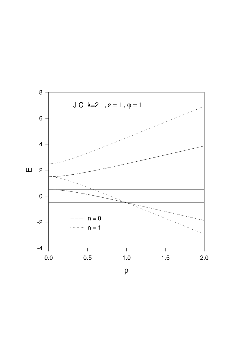
Figure 1: The first few energy levels in the $k=2$-JC Hamiltonian for $\epsilon=1$ and $\phi=1$.

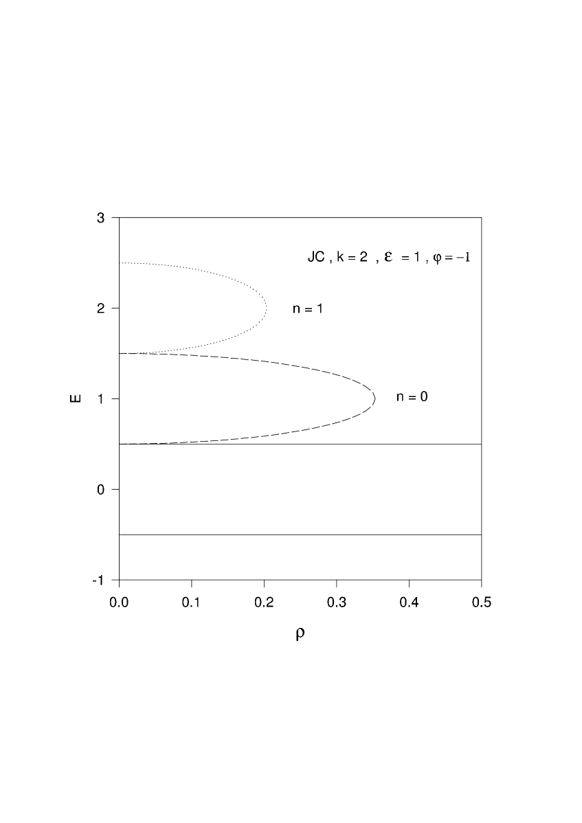
Figure 2: The first few energy levels in the $k=2$-JC Hamiltonian for $\epsilon=1$ and $\phi=-1$.

The spectrum of the JC model (and of its generalisations for $k>1$) varies considerably with the parameter $\rho$. In Fig. 1, we show the evolution of six levels in the $k=2,\phi=1$ case. They correspond to the two $\rho$-independant eigenstates and the ones with $n=0,1$ in Eq.(34). In Fig. 1 and in the following we assume $\epsilon=1$ for simplicity but the features pointed out below remain similar for $\epsilon\neq 1$. The same levels corresponding to the non hermitian case $\phi=-1$ are reported on Fig. 2. The contrast with Fig.1 is obvious. Couples of eigenvalues regularly disappear at finite values of the coupling constants $\rho$. So that, at finite $\rho$ only a finite number of real eigenvalues subsist, the other being real. In this respect, the Hamiltonian is like a quasi exactly solvable operator.

The energy levels displayed on Fig.1 corresponds to the six lowest ones in the limit $\rho=0$. The figure clearly shows that they mix relatively quickly for increasing $\rho$ and that, for instance, eigenvectors involving two or more quanta become the ground state for $\rho\sim 1$.

We have studied the evolution of the spectrum when the QES-extension of the model, $H_{12}=\rho a^{2}+\theta a(1-\frac{1}{N+2}a^{\dagger}a)$ namely characterized by the new coupling constant $\theta$, is progressivel switched on. Notice that the vector $\psi_{0}=(\vec{0}\ ,|0\rangle)^{t}$ is an eigenvector with $E=-\epsilon/2$, irrespectively of $\rho,\theta$

In the case $\rho=0,N=1$ the effect of the new term on the eigenvalues under consideration leads to

$$E=-\frac{1}{2}\ ,\ \ \frac{1}{6}(3\pm 4\theta)\ \ ,\ \ \frac{1}{6}(9\pm 2\sqrt{2})\theta,\ \ \frac{5}{2}$$

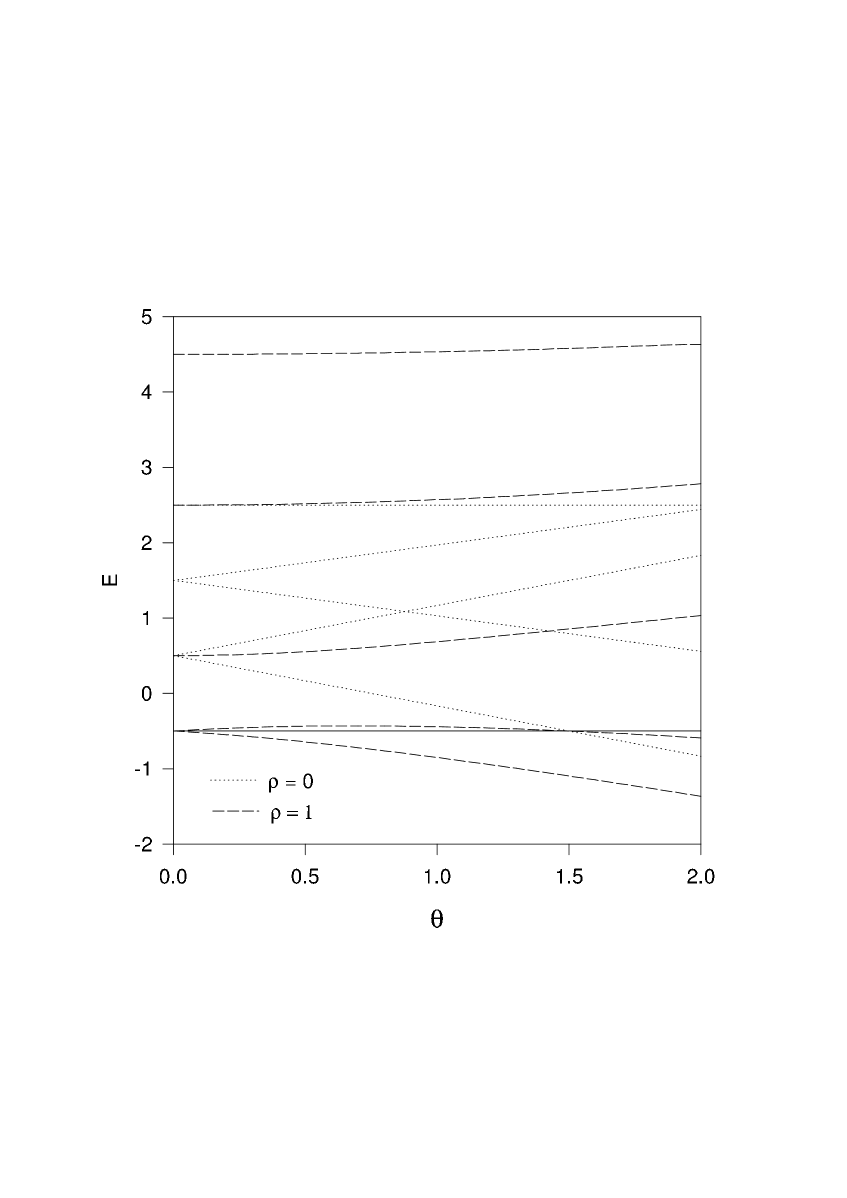
Figure 3: The first few energy levels in the QES deformed $k=2$ JC Hamiltonian as function of the parameter $\theta$, the energy level $E=-1/2$ (solid line) is independant of $\rho$.

These levels are indicated on Fig. 3 by the dotted lines and it is clearly seen that they also lead to numerous level crossing.

The evolution of the eigenvalues corresponding to the case $\rho=1$ is displayed by the dashed lines in Fig.3, supplemented by the black line $E=-1/2$ which is present irrespectively of $\rho$. The figure clearly shows that the occurence of the new term induced only one level mixing, namely two levels cross at $E=-1/2$ for $\theta=1.5$ For larger values of $\rho$, e.g. $\rho=2$, the analysis reveals that the algebraic eigenvalues depend only weakly of $\theta$.

6 Series expansion and Recurence relations

Here we would like to present another aspect of the QES Hamiltonian presented in the previous section. Following the ideas of [15] we will construct the solution for energy $E$ under the form of a formal serie in the basic vector whose coefficients are polynomials in $E$. More precisely, we write the solution of the equation

$$H_{T}\psi=E\psi,$$ (47)

in the form

$$\psi=\left(\matrix{\sum_{j=0}^{\infty}p_{j}(E)\mid j\rangle\cr\sum_{j=-2}^{\infty}q_{j}(E)\mid j+2\rangle\cr}\right)$$ (48)

and where $H_{T}$ is given by the Eq.(41). After some algebra it can be seen that the polynomials $p_{j}(E),q_{j}(E)$ obey the following recurence relations

$$A_{j+1}P_{j+1}+B_{j}P_{j}=0,$$ (49)

where

$$A_{j+1} =\left(\matrix{\rho\sqrt{(j+2)(j+3)}&-(E-(j+1)-\frac{\epsilon}{2})\cr 0&\hat{c}(j+2-n)\sqrt{j+2}\cr}\right),$$ (50)

$$B_{j} =\left(\matrix{c(j+2-n)\sqrt{j+2}&0\cr-(E-(j+2)+\frac{\epsilon}{2})&\rho\sqrt{(j+1)(j+2)}\cr}\right),$$

$$P_{j} =\left(\matrix{q_{j}\cr p_{j}\cr}\right)\ ,\ j=-2,-1,0,1,\dots$$

These equations have to be solved with the initial conditions

$$q_{-2}=0\ ,\ q_{-1}={\cal N}$$ (51)

with ${\cal N}$ fixing the normalisation of the solution. Then the solution for $q_{j}$ turns out to be a polynomial of degree $E^{2j}$. The quasi-exact solvability of the system leads to the fact that $A_{n-1}$ is not invertible and that $p_{n-1}$ can be choosen arbitrarily. With the choice $p_{n-1}=0$ it turns out that all polynomials $p_{j},q_{j}$ with $j\geq n-2$ are proportional to $q_{n-3}(E)$. As a consequence for fixed $n$ and for the values of $E$ such that $q_{n-3}(E)=0$ the serie above is truncated and the set of algebraic eigenvectors are recovered. We would like to stress that series considered in this section are built with the basis vector of the harmonic oscillator and not on monomials in $x$ contrasting with the construction of Ref.[15]. In the case of standard QES equations [15] there it appears a three terms recurence relations which leads to sets of orthogonal relation. In the case of systems of QES equations adressed in [16] the recurence relation is also three terms but the situation here is quite different. Actually, it is to our knowledge, an open question to know whether the set of polynomials $(p_{j}(E),q_{j}(E))$ are somehow orthogonal as it is the case for standard scalar equation.

7 Hidden algebraic structures

As pointed out in the previous sections, the different Hamiltonians studied here posses the property that their spectrum can be (partly or fully) computed. This property is deeply related to the fact that the corresponding operators are elements of the enveloping algebra of particular graded algebra in an appropriate finite dimensional representation. The classification of linear operators preserving the vector spaces ${\cal V}(m,n)=(P_{m}(x),P_{n}(x))^{t}$ was reported in [10]. It is shown that these operators are the elements of the enveloping algebra of some non-linear graded algebra depending essentially of $|m-n|$. Note that, in the present context, the difference $|m-n|$ is nothing else but the parameter called $k$ in Sect. 3. The cases $k=1$ and $k=2$ are special because the underlying algebra is indeed a graded Lie algebra. In the case $k=1$, related to the conventional JC model, the Hamiltonian is an element of the enveloping algebra of $osp(2,2)$; in the representation constucted in [9]. The generators involved in this relation do not depend explicitely on $n$, i.e. of the dimension of the representation, explaining that the Hamiltonian is exactly solvable. Finally, in the case $k=2$, the Hamiltonian is an element of the graded Lie algebra q(2), as shown in [17, 18]. This algebra possesses an sl(2)$\times$U(1) bosonic subalgebra and six fermionic operators splitted into three triplets of the sl(2) subalgebra. In the case of the JC model corresponding to $k=2$, the Hamiltonian is independant on the dimension of the representation $n$ and the model is exactly solvable. For the modified model of Sect. 4, the supplementary interaction term $H_{I}$ defined in (40) indeed depends on $n$ and the operator admit only the vector space ${\cal V}_{n}$ as finite dimensional invariant vector space.

8 Conclusions

In this letter, we have considered several extensions of JCM by adding to its original Hamiltonian the polynomial $P(a^{\dagger}a)$ of degree $d\geq 2$ and an arbitrary sign, say $\phi=\pm 1$, in the non-diagonal interaction term. In fact, considering this sign $\phi=-1$, these extended Hamiltonians are nonhermitian and not PT invariant but they satisfy the pseudo-hermiticity with respect of different operators $P$ and $\sigma_{3}$. This new property reveals the reality of the energy spectrum which has been constructed algebraically. They become hermitian when one considers the sign $\phi=1$. Notice that these Hamiltonians are completely solvable as it has been pointed out by the QES technique.

Several usual properties available with hermitian Hamiltonian are not kep with pseudo-hermitican. Namely the eigenstates given by (27) and (28)(i.e corresponding to the doublet $\mid 0,\frac{1}{2}\rangle$ and $\mid k,-\frac{1}{2}\rangle$) are not orthogonal to each other, but they are orthogonal to all eigenstates corresponding to other doublets. For example, the eigenstate (27) and the one given by Eq.(35)(i.e it corresponds to the doublet $\mid n,\frac{1}{2}\rangle$ and $\mid n+k,-\frac{1}{2}\rangle$) are orthogonal to each other. The eigenstates of any particular doublet are orthogonal to each other only if $\theta_{m}=m\pi$ (i.e with $m=0,1,2,\dots,k,\dots,n+k$), this implies $\rho=0$ because it depends to $\sin\theta_{m}$. In fact, as the energy eigenvalues are entirely real, it is impossible to have all eigenstates orthogonal to each other. This is explained by the unbroken symmetry of the operator $P\sigma_{3}$. But for energy eigenvalues complex, the orthonormality condition is satisfied by all the associated eigenstates. All these discussions are the result of the scalar product applied to those eigenstates.

We manage to construct a JC-type Hamiltonian describing both one and two-photons interactions in terms of quasi exactly solvable operators. This involves a very specific interaction term of degree one in the creators and annihilators which can be seen as a perturbation of more conventional p-photons interacting term. Several properties of this new family of QES-operators have been presented. Namely, (i) they can be written in terms of the generators of the graded Lie algebra osp(2,2) in a suitable representation; (ii) when expressed as series, the formal solutions of $H_{T}\psi=E\psi$ leads to a different type of recurence relation between the different terms of the series.

References

• [1] C. M. Bender and S. Boettcher, Phys. Rev. Lett. 80, 5243(1998); C. M. Bender, S. Boettcher and P. N. Meisinger, J. Math. Phys. 40, 2210(1999).
• [2] C. M. Bender and S. Boettcher, Phys. Rev. Lett. 89, 270401(2002).
• [3] C. M. Bender hep-th/0501052.
• [4] A. Mostafazadeh, J. Math. Phys. 43, 205(2002); 43, 2814(2002); 43, 3944(2002); A. Mostafazadeh and A. Batal, J. Phys. A37, 11645(2004).
• [5] B. P. Mandal, hep-th/0412160 Mod. Phys. Lett A 20 655 (2005).
• [6] P. K. Ghosh, quant-ph/0501087, J. Phys. A 38, 7313 (2005).
• [7] A. Turbiner, Commun. Math. Phys. 119, 467 (1988).
• [8] A.G. Ushveridze, Quasi exactly Solvable Models in Quantum Mechanics (IOP 1995).
• [9] M. Shifman and A. Turbiner, Commun. Math. Phys.
• [10] Y. Brihaye and P. Kosinski, J. Math. Phys. 35 3089 (1994).
• [11] C. C. Gerry, Phys. Rev. A37, 2683(1988).
• [12] B. Deb and D. S. Ray, Phys. Rev.A48, 3191(1993).
• [13] P. L. Knight and P. M. Radmore, Phys. Rev. A26, 676(1982).
• [14] N. Debergh and A.B. Klimov, J.Mod.Phys.Vol.16, 4057(2001).
• [15] C. M. Bender and G. V. Dunne, J.Math. Phys. 37, (1996).
• [16] Y. Brihaye, J. Ndimubandi and B. Prasad Mandal, ”QES polynomials, invariant spaces and polynomials recursion”, math-ph/0601004.
• [17] N. Debergh and J. Van der Jeugt, J. Phys. A 34,
• [18] Y. Brihaye and B. Hartmann, Phys. Lett. A 306, 291