Microwave emission from a crystal of molecular magnets – The role of a resonant cavity

Abstract

We discuss the effects caused by a resonant cavity around a sample of a magnetic molecular crystal (such as Mn₁₂-Ac), when a time dependent external magnetic field is applied parallel to the easy axis of the crystal. We show that the back action of the cavity field on the sample significantly increases the possibility of microwave emission. This radiation process can be supperradiance or a maser-like effect, depending on the strength of the dephasing. Our model provides further insight to the theoretical understanding of the bursts of electromagnetic radiation observed in recent experiments accompanying the resonant quantum tunneling of magnetization. The experimental findings up to now can all be explained as being a maser effect rather than superradiance. The results of our theory scale similarly to the experimental findings, i.e., with increasing sweep rate of the external magnetic field, the emission peaks are shifted towards higher field values.

I Introduction

Magnetic complex molecules have attracted a great deal of attention in recent years, because they have remarkable properties, related to their high magnetic anisotropy and large value of spinBarbara et al. (1999); Wernsdorfer and Sessoli (1999); Villain (2003): for Mn₁₂Ac as well as for Fe₈O, the quantum number of the total spin is $S=10.$ Accordingly, the eigenvalues of $S_{z}$, (the spin component in the direction of the easy axis), can take $21$ different values: $m=-10,\ldots,10.$ One of the most interesting properties of these molecules is that in a slowly changing external magnetic field the magnetization of the crystal consisting of such molecules exhibit series of steps at sufficiently low temperatures.Friedman et al. (1996) The effect can be explained by assuming that the energy levels of the molecules become doubly degenerate at the corresponding values of the magnetic field and this resonance condition increases the possibility of the transition between the degenerate states with different values of $m$ and $m^{\prime}$. This kind of quantum tunneling between spin levels leads to a sudden change in the magnetic moment of the crystal and is therefore of fundamental importance as being a macroscopically observable quantum effect.

In an important theoretical work Chudnovsky and GaraninChudnovsky and Garanin (2002) proposed that resonant magnetic tunneling could be accompanied by the emission of electromagnetic radiation, the possibility of superradiance from magnetic molecules has been considered further in Ref. [Henner and Kaganov, 2003] and bursts of microwave pulses have actually been detected in recent experiments.Tejada et al. (2004); Vanacken et al. (2004); Hernandez-Minguez et al. (2005) According to Refs. [Chudnovsky and Garanin, 2002; Henner and Kaganov, 2003; Joseph et al., 2004], the possible physical mechanism responsible for this phenomenon can be superradiance (SR)Dicke (1954); Benedict et al. (1996); Gross and Haroche (1982) which is an interesting collective effect predicted first by Dicke in 1954, and has been experimentally observed in several physical systems since then.Benedict et al. (1996) However, when the radiation emitted by magnetic molecules was detected, the sample was placed in a container, which acted as a waveguide. This cavity changes the mode structure of the electromagnetic field surrounding the sample, which is known to have crucial effects on the dynamics of the emitted radiation. Studies in SR with other physical systems like the ensemble of proton spins Benedict et al. (1996); Kiselev et al. (1988); Bazhanov et al. (1990); Yukalov and Yukalova (2004) in the MHz, and with Rydberg atoms in the GHz domainHaroche and Raimond (1985) show that the presence of a resonant cavity may enhance the collectivity of the radiating individual dipoles, as first proposed by Bloembergen and Pound Bloembergen and Pound (1954), and which seems to be necessary to obtain radiation in the case of molecular magnets, as well.Yukalov and Yukalova (2005a, b) Additionally, it has also been demonstrated that external resonators such as Fabry-Perot mirrors can enhance the relaxation of a crystal of molecular nanomagnets.Tejada et al. (2003) Inspired by these facts, we investigate in this paper the interplay between the radiation and the changes of the magnetization of a macroscopic sample of molecules Mn₁₂-Ac inside a nearly resonant cavity. We also note that the interesting proposal of Ref. [Leuenberger and Loss, 2001] to use these molecules for implementing a quantum algorithm gives another motivation to study their radiative properties.

The present paper is organized as follows: In Sec. II we investigate the relevant magnetic level structure and describe a method that allows us to reduce the problem to a set of level pairs. The interaction of the molecules with the cavity field is considered in Sec. III. In Sec. IV we discuss the approximate analytical consequences of our model and present numerical results as well. Finally we summarize and draw the conclusions (Sec. V).

II Magnetic level structure

Experiments including magnetization measurements, Friedman et al. (1996); Mertes et al. (2001) neutronMirebeau et al. (1999) and EPRBarra et al. (1997); Hill et al. (1998, 2003) studies on crystals of Mn₁₂Ac and Fe₈O suggest that the Hamiltonian responsible for the magnetic properties can be written as a sum of two terms:

$$H_{S}=H_{0}+H_{1}.$$ (1)

Here $H_{0}$ is diagonal in the eigenbasis $\{|m\rangle\}$ of the (dimensionless) $z$ component of the spin operator, $S_{z}$:

$$H_{0}=-DS_{z}^{2}-FS_{z}^{4}-\tilde{\mu}B_{0}S_{z},$$ (2)

where the last term describes the coupling to an external magnetic field applied in the $z$ direction (easy axis): $\mathbf{B}_{0}=(0,0,B_{0})$ with $\tilde{\mu}=g\mu_{B}$. On the other hand, $H_{1}$ consists of termsMertes et al. (2001); Barra et al. (1997) that do not commute with $S_{z}$:

$$H_{1}=C(S_{+}^{4}+S_{-}^{4})+E(S_{+}^{2}+S_{-}^{2})/2+K(S_{+}+S_{-})/2.$$ (3)

As most of the experiments where microwave radiation emitted by magnetic molecules was detected have been performed on Mn₁₂-Ac, from now on, we shall consider this molecule as the representative example. In this case the values of the parameters in $H_{0}$ are $D/k_{B}=0.56K,$ and $F/k_{B}=1.1\cdot 10^{-3}K$. The coefficients in $H_{1}$ do not have unanimously accepted values, but $H_{1}$ can be considered as a small correction to $H_{0}$. However, as the transitions between levels with different $m$ and $m^{\prime}$ are induced by terms that do not commute with $S_{z}$, the importance of $H_{1}$ is fundamental from this point of view. Tetragonal symmetry would allow only the quartic term, but there is experimental evidenceMertes et al. (2001) showing the presence of weak quadratic and linear terms in $H_{1}$. We shall return to the determination of the coefficients in $H_{1}$ at the end of this section.

In a typical experimental situation the external field $B_{0}$ slowly changes in time, and consequently so does $H_{0}$. Considering the total Hamiltonian (1) as the generator of the time evolution (which means that relaxation effects are not taken into account), the corresponding time dependent Schrödinger equation governs the dynamics. However, it turns out that its solution is not feasible, because the time independent part of $H_{0}$ forces a much faster evolution than the slow variation due to the change of the magnetic field. The fundamental frequencies $\omega_{mm^{\prime}}\approx(D/\hbar)(m^{\prime 2}-m^{2})$ are in the range $10^{10}-10^{11}s^{-1}$ being very fast compared with the time dependence of the magnetic field $B_{0}$ that among ordinary circumstancesTejada et al. (2004) cause a change on the scale $10s^{-1}$. Therefore there is a significant variation in the molecular state as a consequence of the first term in (2), while nothing happens due to $-\tilde{\mu}B_{0}S_{z}$, which appears in the last term of $H_{0}$. On the other hand, we know that an appreciable change in the state occurs only if two energy levels become close to each other, as stipulated by a simple time dependent perturbation calculation, where the energy difference between the levels appears in the denominator of the transition probability. As the dominant term in the Hamiltonian (1) is $H_{0}$, we can approximately find the points where two energy levels are close to each other by calculating the eigenvalues of $H_{0}$, which are obtained by the mere substitution $S_{z}\rightarrow m$. Simple algebra shows that these eigenvalues become doubly degenerate with given $m$ and $m^{\prime}$ at the following values of $B_{0}$:

$$\tilde{\mu}B_{0}=-D(m+m^{\prime})\left(1+\frac{F}{D}\left[m^{2}+m^{\prime 2}\right]\right).$$ (4)

A part of the level scheme of the total Hamiltonian $H_{S}$ is shown in Fig. 1 as function of $B_{0}$. The special values of $B_{0}$ given by Eq. (4) – where the levels of $H_{0}$ cross – can be clearly identified in this figure. However, as it is known, the presence of $H_{1}$ perturbs the eigenvalues leading to a splitting of the levels instead of crossing as shown by the inset. The resonance condition implies that appreciable changes in the population of the levels is expected around these avoided crossings (sometimes also called anticrossings). Thus the system can be efficiently approximated by a set of level pairs, each of which is to be considered as an effective two-level system, similarly to the figure shown in the inset.

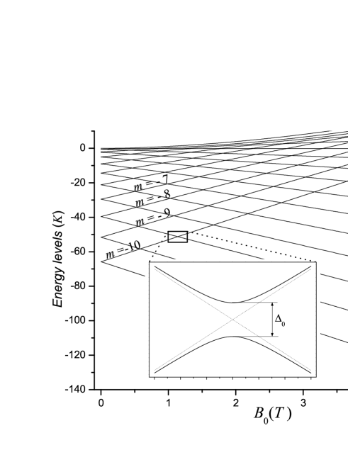
Figure 1: The energy levels of Hamiltonian (1) as a function of the external magnetic field $B_{0}$. The parameters are $D/k_{B}=0.56K,$ $F/k_{B}=1.1\cdot 10^{-3}K,$ $K=0.025\tilde{\mu}B_{0}$, $E/k_{B}=-4.48$ $10^{-3}$ $K$ and $C/k_{B}=1.36$ $10^{-5}$ $K.$ The inset zooms on the vicinity of $B_{0}=1.13$ T, where – due to the presence of $H_{1}$ – we can see a level splitting of $\Delta_{0}$ between the levels $m=-10$ and $m^{\prime}=8$.

Reducing the problem to a set of level pairs means technically that one applies degenerate perturbation theory around each avoided level crossing (determined by the values of $B_{0}$ in Eq. (4)) following a technique proposed independently by van Vleckvan Vleck (1929), Des Cloiseauxdes Cloizeaux (1960) and other authors as summarized in Ref. [Klein, 1974]. In the vicinity of a given avoided level crossing we find a unitary transformation that block diagonalizes $H_{S}$ on the zero order two-dimensional eigensubspaces and generate an effective Hamiltonian $H_{e}$ that has the same eigenvalues as $H_{S}$:

$$H_{e}=UH_{S}U^{\dagger}$$ (5)

with

$$U=\sum_{a}(P_{a}^{0}P_{a}P_{a}^{0})^{-1/2}P_{a}^{0}P_{a},$$ (6)

where $a$ labels the various eigensubspaces with quasi-degenerate eigenvalues, and $P_{a}^{0}$ are orthogonal projections on the degenerate eigensubspaces of $H_{0}$. For a given value of $a,$ corresponding to the avoided crossing of levels $m$ and $m^{\prime}$, we have $P^{0}=|m\rangle\langle m|+|m^{\prime}\rangle\langle m^{\prime}|.$ As the perturbation is turned on, the $\{\left|m\right\rangle,\left|m^{\prime}\right\rangle\}$ eigenstates of $H_{0}$ evolve into $\{\left|\phi_{m}\right\rangle,\left|\phi_{m^{\prime}}\right\rangle\}$ and we consider $P=|\phi_{m}\rangle\langle\phi_{m}|+|\phi_{m^{\prime}}\rangle\langle\phi_{m^{\prime}}|$ which projects onto the space arising from the zero order subspace of interest. By appropriate expansionsGaranin (1991); Leuenberger and Loss (2000); Yoo and Park (2005) of this unitary operator $U$, one can obtain a perturbation series, leading to useful analytical approximations of $H_{e}.$ Alternatively, the numerically exact projections $P_{a}$ can be found by the diagonalization of $H_{S}$, and then Eqs. (5) and (6) provide the operator $H_{e}$. The latter method is followed in this paper and we obtain in each two-dimensional subspace spanned by $\{\left|m\right\rangle,\left|m^{\prime}\right\rangle\}$ the following matrix for the effective Hamiltonian:

$$H_{e}(t)=\left(\begin{array}[]{cc}\varepsilon_{0}+w/2&\Delta_{0}/2\\ \Delta_{0}/2&\varepsilon_{0}-w/2\end{array}\right)_{m,m^{\prime}}$$ (7)

with time dependent elements, and of course the values depend also on the pair $\{\left|m\right\rangle,\left|m^{\prime}\right\rangle\}$. Here $\varepsilon_{0}$ is the energy where the given crossing would occur, $w$ is proportional to the time dependent external field in the $z$ direction, while the offdiagonal element $\Delta_{0}$ is the level splitting responsible for the effective coupling between the levels. $w$ will be assumed to be linear in time with constant $\dot{B}_{0}$, yielding $w(t)=-\tilde{\mu}\dot{B}_{0}(t-t_{0})(m-m^{\prime})$ with $t_{0}$ being the time instant when the crossing would occur. Note that this is a reasonable approximation even for a time scale much longer than the expected duration of the transition to be described (see e.g. Fig. 1. in Ref. [Vanacken et al., 2004]). This linear approximation corresponds to the usual Landau-Zener-Stückelberg (LZS) model Landau (1932); Zener (1932); Stückelberg (1932), by the aid of which we can calculate the probability of a given $m\rightarrow m^{\prime}$ transition: $P_{mm^{\prime}}=1-\exp(-\pi\Delta_{0}^{2}/2\hbar w)$. Note that in this expression both $w$ and $\Delta_{0}$ depend on the labels $m,m^{\prime}$. For a given pair of levels and sweep rate $\dot{B}_{0}$, $P_{m,m^{\prime}}$ is determined by the magnitude of the level splitting $\Delta_{0}$, i.e., essentially by the parameters in $H_{1}$. If we assume that initially the system is in thermal equilibrium, we can consider a series of transitions at the values of $B_{0}$ given by Eq. (4). Calculating the expectation value of the operator $S_{z}$ (which is proportional to the magnetization) we obtain a staircase-like hysteresis loop that can be compared with the experimental curvesMertes et al. (2001) at a given temperature and sweep rate. As our results depend on the coefficients in $H_{1}$, the minimization of the difference between the steps in the calculated hysteresis curve and the experimental plots gives the desired parameter values. We have found the best agreement for $K=0.025\tilde{\mu}B_{0}$, $E/k_{B}=-4.48$ $10^{-3}$ $K$, $C/k_{B}=1.36$ $10^{-5}$ $K$, therefore these parameter values will be used in the following.

The method summarized in this section, first of all, gives us information about the magnitude of the terms in the spin Hamiltonian, and describes how to obtain the level splittings $\Delta_{0}$. As we shall see in the next section, the coupling of the molecular system to the cavity field at a given $m\rightarrow m^{\prime}$ transition can also be determined in this way.

III Interaction with the resonant cavity field

In this section we describe the interaction of an ensemble of magnetic molecules with a quasi-resonant cavity field. The time dependence of the level structure, considered in the previous section, will bring a certain level pair into resonance with the cavity field at a given value of the external magnetic field $\mathbf{B}_{0}.$ Usually there are avoided level crossings before the resonance, where for low lying $m$ and $m^{\prime}$ the LZS transition probabilities $P_{m,m^{\prime}}$ are small, leading to an almost complete inversion. We shall consider a dynamical equation for the density operator of the molecules and assume that a dipole moment is generated during a certain transition between the split levels $m$ and $m^{\prime}$ of a given molecule which in turn serves as a source of microwave radiation influencing the transitions in all other molecules. To take into account this radiation mediated interaction, we have to add a new term to the effective two-level Hamiltonian describing the interaction with the magnetic dipole field of the cavity, $\mathcal{\vec{B}}$, which is an additional field beyond the stronger but almost static magnetic field $\mathbf{B}_{0}$ creating the inversion between the levels. The fast dynamics of the magnetic dipoles will be a forced oscillation generated by the interaction with the external field that is characterized by the interaction Hamiltonian $H_{I}=\tilde{\mu}\mathcal{\vec{B}}\mathbf{\tilde{S}}_{e}.$ Here $\mathbf{\tilde{S}}_{e}=USU^{\dagger}=(\tilde{S}_{x},\tilde{S}_{y},\tilde{S}_{z})$ denotes the spin operator one obtains after the unitary transformation (5) described in the previous section, by restricting it to the actual two-dimensional subspace we consider. The matrix elements of $\mathbf{\tilde{S}}_{e}$ usually differ from those of $\mathbf{S.}$ As for the field strength $\mathcal{\vec{B}},$ a detailed model should take into account the mode structure of the cavity. However, the characteristic features of the dynamics due to the cavity field can be captured by a simpler model to be discussed here. We consider the microwave field as a single transverse (TM) mode being perpendicular to the $z$ (easy) axis and having a frequency $\Omega$ and equal amplitudes in the $x$ and $y$ directions: $H_{I}=-\tilde{\mu}\mathcal{B}(\tilde{S}_{x}+\tilde{S}_{y})/\sqrt{2}$. We note that the choice of the polarization does not have essential influence on the results presented here. Now the equations describing the dynamics of the two-level system (without relaxation) can be written as

$$\frac{\partial\varrho}{\partial t}=-\frac{i}{\hbar}\left[H^{\prime},\varrho\right],$$ (8)

where $\varrho$ is the density operator of the effective two-level system and

$$H^{\prime}=H_{e}+H_{I}=\left(\begin{array}[]{cc}\varepsilon_{0}+\hbar\omega/2&\Delta/2\\ \Delta^{\ast}/2&\varepsilon_{0}-\hbar\omega/2\end{array}\right)_{mm^{\prime}}.$$ (9)

Here $\hbar\omega(t)=w(t)-2\tilde{\mu}\mathcal{B}s^{\prime}$ and $\Delta=\Delta_{0}-2\tilde{\mu}\mathcal{B}s$ with $s^{\prime}$ and $s$ being the diagonal and offdiagonal elements resulting from the coupling operator $(\tilde{S}_{x}+\tilde{S}_{y})/\sqrt{2}$. This leads to the following equations for the population differences and the coherences between the states:

$$\frac{d}{dt}(\varrho_{mm}-\varrho_{m^{\prime}m^{\prime}}) = \frac{i}{\hbar}(\Delta^{\ast}\varrho_{mm^{\prime}}-\Delta\varrho_{m^{\prime}m})$$ (10)

$$\frac{d}{dt}\varrho_{mm^{\prime}} = -i\omega(t)\varrho_{mm^{\prime}}+\frac{i}{2\hbar}\Delta(\varrho_{mm}-\varrho_{m^{\prime}m^{\prime}}).$$ (11)

As $\Omega$ is in the terahertz domain, we can separate a slowly varying amplitude of the time varying field and write

$$\mathcal{B}=\left(\frac{1}{2}B(t)e^{-i\Omega t}+c.c.\right)u_{k}(z),$$ (12)

where $u_{k}(z)$ is the corresponding mode function of the cavity, and $\left|\dot{B}(t)\right|\ll\Omega\left|B\right|$. This makes straightforward a similar separation for the offdiagonal elements of the density matrix: $\varrho_{mm^{\prime}}=R_{mm^{\prime}}e^{-i\Omega t}$ where $R_{mm^{\prime}}$ is again assumed to vary slowly compared with $e^{-i\Omega t}.$ Substituting into Eq. (10) we can neglect terms oscillating with frequency $2\Omega$ as they do not contribute essentially to the evolution of the state, i.e, this is the standard rotating wave approximation (RWA)Sargent et al. (1974). Introducing the notation $Z_{mm^{\prime}}=\varrho_{mm}-\varrho_{m^{\prime}m^{\prime}}$ for the inversion between levels $m$ and $m^{\prime}$, we obtain:

$$\frac{d}{dt}Z_{mm^{\prime}} = \frac{i}{2\hbar}\left\{\left(R_{mm^{\prime}}\Delta_{0}^{\ast}e^{-i\Omega t}-R_{mm^{\prime}}^{\ast}\Delta_{0}e^{i\Omega t}\right)-\tilde{\mu}(B^{\ast}s_{mm^{\prime}}^{\ast}R_{mm^{\prime}}-Bs_{mm^{\prime}}R_{mm^{\prime}}^{\ast})u_{k}^{2}(z)\right\}$$ (13)

$$\frac{d}{dt}R_{mm^{\prime}} = -i(\omega(t)-\Omega)R_{mm^{\prime}}+\frac{i}{\hbar}(\Delta_{0}e^{i\Omega t}-\tilde{\mu}Bs_{mm^{\prime}})Z_{mm^{\prime}}\text{.}$$ (14)

At a given time instant only one of the level pairs get into resonance with the cavity, therefore from now on we shall omit the indices $m,m^{\prime}$. We shall come back to this point, and discuss the mechanism which selects the actual level pair. We can also average out the equations over a time period of a cycle of the oscillation that eliminates the terms varying with frequency $\Omega$. A similar procedure can be performed in space over the wavelength $\lambda=2\pi/k$, and we shall make use of $\frac{1}{\lambda}\int_{0}^{\lambda}u_{k}^{2}(z)=1/2$.

We also have to describe the effects caused by other degrees of freedom. These additional interactions – among which the strongest one is the spin phonon coupling, i.e, the oscillation of the atoms in the lattice – are not taken into account by the Hamiltonian (1), but can significantly influence the dynamics. The effects due to the reservoir of phonons (i) can be dissipative, by simply taking up the energy from the spin system and (ii) dephasing, by randomly disturbing the relative phases of the magnetic states. Dissipative terms lead to a decay of the diagonal elements while dephasing reduce the off-diagonal elements of $\mathcal{\varrho}$. The diagonal terms relax generally much slower than the offdiagonal ones, therefore we consider only this (so called transversal) relaxation. As usual, it will be taken into account by assuming a simple exponential decay with a time constant $T_{2}$, the order of magnitude of which can be estimated between $10^{-5}$ and $10^{-7}$ s in the temperature range we are interested inLeuenberger and Loss (2000). With this term we have:

$$\frac{d}{dt}Z = -\frac{i\tilde{\mu}}{2\hbar}(B^{\ast}s^{\ast}R-BsR^{\ast}),$$ (15)

$$\frac{d}{dt}R = -i(\omega(t)-\Omega)R-\frac{i}{2\hbar}\tilde{\mu}BsZ-R/T_{2}.$$ (16)

These equations are familiar from the theory of magnetic resonance, and as it is known, the effect of the field $B$ is essential when the frequency originating from the slowly varying longitudinal field gets close to the cavity frequency: $\omega(t)\approx\Omega$.

We also treat the mode amplitude of the cavity as a dynamical quantity. Following the usual semiclassical approach of radiation-matter interaction theorySargent et al. (1974), the time varying field resulting from the magnetic molecules of the crystal will be described here as the field of a sample with time dependent magnetic dipole moment density $\mathcal{M}$ in the $x-y$ plane. The appropriate component of the transverse $\mathcal{H}$ field originating from $\mathcal{M}$ as a source, obeys the damped inhomogeneous wave equation

$$\Delta\mathcal{H}-\mathcal{\dot{H}}/(c^{2}T_{c})\mathcal{-}\ddot{\mathcal{H}}/c^{2}=\ddot{\mathcal{M}}/c^{2},$$ (17)

where $T_{c}$ is the cavity lifetime. Within the cavity we expand the field into modes, and in accordance with Eq. (12), we also write:

$$\mathcal{H=}\left(\frac{1}{2}He^{-i\Omega t}+c.c.\right)u_{k}(z),\quad\mathcal{M=}\left(\frac{1}{2}Me^{-i\Omega t}+c.c.\right)f(z)$$ (18)

where $f(z)$ is nonzero only within the sample, where it can be taken equal to $u_{k}(z)$. If one substitutes into Eq. (17), and makes an approximation exploiting that the amplitudes, $H$ and $M$ are slowly varyingSargent et al. (1974) with respect to $e^{-i\Omega t}$, one obtains the equation

$$\frac{dH}{dt}=i\Omega\eta\frac{M}{2}-\frac{1}{2T_{c}}H.$$ (19)

The filling factor

$$\eta=\int_{\mathcal{C}}u_{k}(z)f(z)dz/\int_{\mathcal{C}}u_{k}^{2}(z)dz\approx l/L$$ (20)

arises when we project the resulting equation on the mode in question, by integrating over the volume of the cavity. Here $l/L$ is the ratio of the lengths of the sample and the cavity, corresponding to the geometries reported in the experimentsTejada et al. (2004); Vanacken et al. (2004).

The corresponding component of the transverse magnetization of the sample is given by

$$\mathcal{M}=N_{0}\tilde{\mu}Tr\left[\varrho(\tilde{S}_{x}+\tilde{S}_{y})/\sqrt{2}\right]=N_{0}\tilde{\mu}(s^{\ast}\varrho_{mm^{\prime}}+s\varrho_{m^{\prime}m}),$$ (21)

where $N_{0}$ is the number density of the molecules participating in the transition $m\rightarrow m^{\prime}$. We note that the static part of $\mathcal{M}$ containing $s^{\prime},$ does not give rise to radiation. Eq. (21) connects the microscopic dynamical variables with the macroscopic ones. Recalling that $\varrho_{mm^{\prime}}=R_{mm^{\prime}}e^{-i\Omega t}$, we see that $M=2N_{0}\tilde{\mu}s^{\ast}R_{mm^{\prime}}.$ The slowly varying magnetic induction field acting on the molecules is given by $B=\mu_{0}(H+\beta M)$, where $\mu_{0}$ is the vacuum permeability and $\beta$ may differ from unity giving account of a local field correction resulting from the near field of the dipolesJackson (1998). It is natural to measure the time variable in units of the characteristic time

$$T_{0}=\left(\frac{2\hbar}{\eta N_{0}\Omega\mu_{0}\tilde{\mu}^{2}\left|s\right|^{2}}\right)^{1/2}.$$ (22)

As we shall see, the relation of $T_{0}$ and the rate of relaxation characterizes the dynamics: in case of $T_{0}/T_{2}\ll 1$ the phase correlation of the individual emitters is conserved during the process and a superradiant pulse (or a sequence of pulses) can be emitted. On the other hand, $T_{0}/T_{2}>1$ indicates that relaxation effects are too strong to allow SR to occur.

To perform the calculations it is straightforward to introduce the dimensionless magnetic field strength and induction amplitudes:

$$h=\left(\frac{\mu_{0}}{N_{0}\hbar\Omega}\right)^{1/2}H,\quad\text{ \ }b=\left(\frac{1}{\mu_{0}N_{0}\hbar\Omega}\right)^{1/2}B.$$ (23)

The field intensity can be measured as the energy density averaged out over the time and space period. The dimensionless field intensity $I=\left|h\right|^{2}/2$ gives the number of emitted photons of energy $\hbar\Omega$ per number of molecules participating in the given transition. Outside the sample $h=b,$ while within the sample one has

$$b=h+2\beta\frac{1}{\eta T_{0}\Omega}Re^{-i\psi},$$ (24)

where $\psi$ is the phase of the offdiagonal coupling constant: $s=|s|e^{i\psi}$. The dynamical equation for the magnetic field in dimensionless form reads:

$$\frac{dh}{d\tau}=-\frac{\kappa}{2}h+iRe^{-i\psi},$$ (25)

where $\tau=t/T_{0}$ and $\kappa=(T_{0}/T_{c}),$ is the damping coefficient of the cavity. These equations are to be solved together with Eqs. (15,16), which take the dimensionless form:

$$\frac{d}{d\tau}Z = -i(b^{\ast}Re^{-i\psi}-bR^{\ast}e^{i\psi}),$$ (26)

$$\frac{d}{d\tau}R = -iT_{0}(\omega(\tau)-\Omega)R-ibe^{i\psi}Z-\gamma R.$$ (27)

with $\gamma=T_{0}/T_{2}$. Note that numerically (using SI units) $T_{0}\approx|s|^{-1}\times 10^{-8}s$, where we substituted $N_{0}\eta=10^{23}m^{-3}$, corresponding to the values reported in the experimentTejada et al. (2004). Depending on the transition $m\rightarrow m^{\prime}$, usually the magnitude of the dimensionless matrix element $|s|$ is much less than unity, thus $10ns$ (obtained with $|s|=1$) is basically a lower bound for $T_{0}$. This value – at least at low temperatures – is less than the time scale of the relaxation, $T_{2}$, but clearly by orders of magnitude larger than the period of the microwave radiation $1/\Omega$, thus our rotating wave approximation leading to Eqs. (15,16) is valid. Additionally, as $\Omega$ is around $10^{11}$ $s^{-1}$, Eq. (24) shows that it is a very good assumption to take $h=b$ within the sample as well.

IV Results and Discussion

The generic scheme for the emission from the ensemble of magnetic molecules considered in this paper starts with inverted two-level systems that come into resonance with the cavity field at a certain value of the external magnetic field $B_{0}$. Besides resonance, an additional requirement for the transverse radiation to begin is that the wavelength corresponding to the transition frequency should be comparable or smaller than the size of the sample, otherwise the non-transverse near-field of the sources would dominate the emitted field at the location of the other molecules. This explains why in the experiments reported in Ref. [Tejada et al., 2004] the emission is in the $mm$ range wavelength.

Now we shall analyze if the observed radiation can be considered as superradiance demanding $\gamma\ll 1$, or is it rather a maser effect, where the absence of phase relaxation is not crucial. Therefore we first assume that $\gamma=0,$ and  see that equations (26) and (27) admit a simple constant of motion:

$$Z^{2}+2\left|R\right|^{2}=Z_{0}^{2}.$$ (28)

If $\omega(\tau)$ is changing sufficiently slowly, the condition of resonance $\omega(\tau)-\Omega_{c}=0$ is sustained during the dynamics of the emission. Then writing $Z=Z_{0}\cos\theta(\tau)$, and $\left|R\right|=(Z_{0}/\sqrt{2})\sin\theta(\tau)$, a simple equation yielding essential physical insight into the nature of the problem can be obtained. With the assumptions that $R$ is real, $\psi=\pi/2$ and using Eqs. (26,27), one has $b=\frac{d}{d\tau}\theta(\tau)/\sqrt{2}\equiv\dot{\theta}/\sqrt{2}$, and from Eq. (25) we obtain

$$\ddot{\theta}(\tau)+\kappa\dot{\theta}(\tau)/2-Z_{0}\sin\theta(\tau)=0,$$ (29)

which is the equation of a damped pendulum ($\theta$ measured from the inverted position), being often discussed in coherent atom-field interactions. The physically realistic initial condition for $\theta_{0}$ is a small ($\theta_{0}\approx 0$) value, as initially we expect the offdiagonal element of the density matrix to be small. This comes from the small initial polarization as a remnant of the coherence between the levels during the magnetic tunneling transition. Putting in such an initial condition takes into account the rapidly varying terms omitted in Eqs. (14) and (13) which would also lead to a small but nonzero $R$ initially. Experimental results reported in Ref. [Tejada et al., 2004] suggest that the radiation appears after a crossing with small tunneling probability $P_{mm^{\prime}}$, thus there is a significant inversion present in the system, meaning $Z_{0}\approx 1$ in the beginning of the radiation process.

If the cavity lifetime is short, $\kappa$ is large, the second term dominates over the first in Eq. (29). Neglecting $\ddot{\theta},$ the equation of the overdamped pendulum admits an analytical solution. For the emitted intensity one obtains

$$\left|b\right|^{2}=\dot{\theta}^{2}(\tau)/2=\frac{1}{2\tau_{R}^{2}}\mathrm{sech}^{2}[(\tau-\tau_{d})/\tau_{R}],$$ (30)

where $\tau_{R}=\frac{\kappa}{2Z_{0}}$, and $\tau_{d}=\tau_{R}(\ln\theta_{0}/2)$. In this bad cavity limit $T_{c}$ can be estimated as $L/c,\$the time needed for a photon to leave the cavity of length $L$. Assuming $Z_{0}=1$, the characteristic time of the emission in usual units is given by $T_{R}=T_{0}\tau_{R}=T_{0}^{2}\frac{c}{2L}=\frac{\hbar c}{\eta LN_{0}\Omega_{c}\mu_{0}\tilde{\mu}^{2}\left|s\right|^{2}}$. We see that this time constant is inversely proportional to the number density of the molecules, $N_{0}$, while according to Eq. (30), the intensity of the radiation is proportional to $N_{0}^{2}$: these are the characteristic features of superradiance Benedict et al. (1996). In addition, there is a delay time $T_{d}=\tau_{d}T_{0}$ necessary for the appearance of the pulse described in Eq. (30).

In the case the cavity losses do not dominate the process, the energy of the field is fed back into the crystal and according to Eq. (29) this leads to a damped periodic process. Assuming a perfect cavity one has a kind of Rabi oscillations with a time dependent field: energy is exchanged periodically between the crystal and the field.

These considerations based on the analytic solutions, however, become only valid approximately, as they do not take into account the factor $\omega(\tau)-\Omega_{c}$ in Eq. (27). As we assume a constant $\dot{B}_{0}$, we can introduce a constant dimensionless external field sweep rate $v$ via

$$T_{0}(\omega(\tau)-\Omega_{c})=v\tau,$$ (31)

where the origin of the time axis is chosen so that $\tau=0$ corresponds to exact resonance: $\omega(0)=\Omega_{c}$. As an example, at the $m=-10\rightarrow m^{\prime}=8$ transition with $\dot{B}_{0}=30$ mT/s and $T_{0}=10^{-6}s$ we have $v=T_{0}^{2}\tilde{\mu}\dot{B}_{0}(m-m^{\prime})/\hbar\approx 0.1$, leading to a dynamics significantly different from the analytical solution.

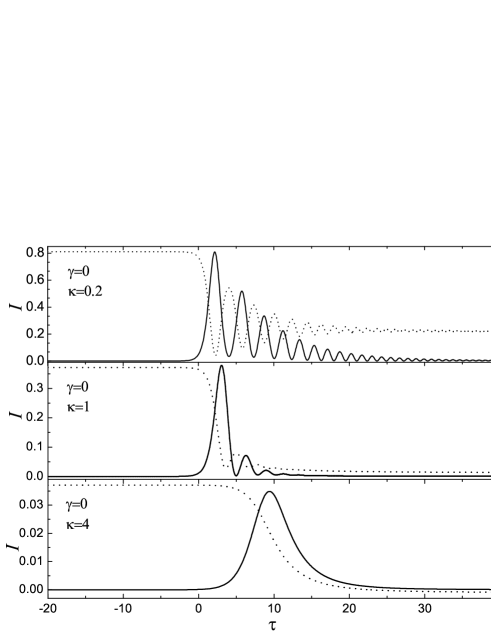
Figure 2: Population difference $Z$ (dotted line) and the dimensionless intensity (solid line) of the radiation emitted by the molecular system as a function of $\tau$ for different cavity decay rates. The transversal relaxation rate $\gamma=0$ and the dimensionless sweep rate corresponding to these plots is $v=0.2$. Note that the energy per unit volume that corresponds to the field $I=1$ means that each active molecule in the sample emits a photon of energy $\hbar\Omega.$

Qualitatively, we expect that around $\tau=0$ (crossing point) the coupling begins to act, and creates a superposition of the levels. The coherence of the levels begin to increase accompanied by a finite transition probability: $Z$ will differ substantially from $Z(-\infty).$ Then the oscillation of the pendulum, i.e., the radiation starts, but as the levels separate, their energy difference and therefore the oscillation frequency becomes larger. Taking relaxation into account, the amplitude of these oscillations diminishes, the molecules do not emit radiation any longer and simultaneously $Z$ will reach a stationary value $Z(\infty),$ analogously to what is usually called quantum tunneling of magnetization, because a different $Z$ means different value of the expectation value of $S_{z}.$ In this sense the inclusion of this time dependent detuning leads to a similar effect as discussed in the problem of tunneling, but the resonance condition is ensured by the inclusion of the time dependent cavity field, therefore the dynamics is more complicated than in LZS theory.

Quantitatively, Fig. 2 shows the inversion and the intensity of the emitted radiation as a function of time for different strengths of the cavity decay. The effect of the resonance is clear, appreciable radiation and change in $Z$ is seen after $\tau=0$. As the cavity damping becomes stronger we have less oscillations in the emitted intensity and the process starts later. For small values of $\kappa$ the final inversion $Z(\infty)$ is determined by the sweep rate, but when cavity losses become significant, the energy of the molecular system is lost via the cavity field during the process leading to $Z(\infty)\approx-1$. A bad cavity ($\kappa\gg 1$) overdamps the pendulum and the system leaves the vicinity of the resonance before observable emission occurs. We note that the inversion $Z(\infty)$ is not necessarily closely related to the final magnetization of the sample, because following the photon emission, cascade (not purely two-level) transitions related to a given side of the two-well potential can also have a considerable probability.

Figure 3: The effects of the transversal relaxation on the dynamics of the population difference $Z$ (dotted line) and the intensity (solid line) of the radiation emitted by the molecular system. In comparison to Fig. 2, note the saturation effect in $Z$: for a given sweep rate (in this case $v=0.2$) increasing values of $\gamma$ push the final population difference towards positive values.

So far it has been assumed that the phase memory of the system is conserved, $\gamma=T_{0}/T_{2}$ is small and accordingly the damping term $-\gamma R$ was neglected in Eq. (27). This was the assumption that led to the coherent behavior of the molecules resulting in superradiant emission. However, in reality there are at least two reasons to consider nonzero $\gamma$. One of them is the spin-phonon coupling which is temperature dependent, thus can be reduced by cooling the sample. Additionally, if the size of the system is smaller than the wavelength the near field dipole-dipole coupling between the molecules becomes important and can be shown to lead to an effective phase relaxation.Gross and Haroche (1982); Friedberg et al. (1973) Microscopic studies of the latter effect can be found in Refs. [Benedict et al., 1996; Zaitsev et al., 1983], for a detailed recent work see Ref. [Davis et al., 2005]. At very low temperatures this effect can be even stronger than the homogeneous broadening mechanism caused by elastic collisions with the phonons. At temperatures around $2$K, however, where the experiments observing the radiation have been performed, the dephasing is predominantly due to spin-phonon interactions instead of dipole-dipole coupling.Sessoli (1995); Leuenberger and Loss (1999) In the present work all these relaxation mechanisms are incorporated effectively by an appropriately chosen damping coefficient $\gamma$.

The consequences of phase relaxation is shown in Fig. 3, where a moderate constant cavity decay ($\kappa=0.2$) is also taken into account. For weak dephasing, we have similar oscillations in $Z$ and pulse structure as shown in Fig. 2. Increasing the value of $\gamma$ the coherent Rabi oscillations disappear. Additionally, the final inversion $Z(\infty)$ is a monotonically increasing function of $\gamma$, and this can be considered as a remarkable difference between the two decay mechanisms. Note that this saturation effect can be responsible for the additional steps in the hysteresis curve published in Ref. [Tejada et al., 2004] following the most pronounced one which is accompanied by microwave radiation: The nonzero population that remains on the upper level after the transition can lead to an observable change of the magnetization of the sample at a next avoided level crossing.

In the case of strong dephasing, the time derivative of $R$ can be neglected with respect of $\gamma R,$ and from Eq. (27) we obtain that $R$ follows adiabatically the time dependence of $b$. Substituting back into Eq. (26) we obtain the following rate equation description of the process:

$$\frac{dZ}{d\tau} = -Z\left|b\right|^{2}\frac{2\gamma}{\gamma^{2}+v^{2}\tau^{2}},$$

$$\frac{db}{d\tau} = -\frac{\kappa}{2}b+\frac{bZ}{\gamma+iv\tau}.$$ (32)

Here atomic coherence does not play any role, thus the process cannot be termed as superradiance, it is rather a maser, operating on the inverted magnetic levels.

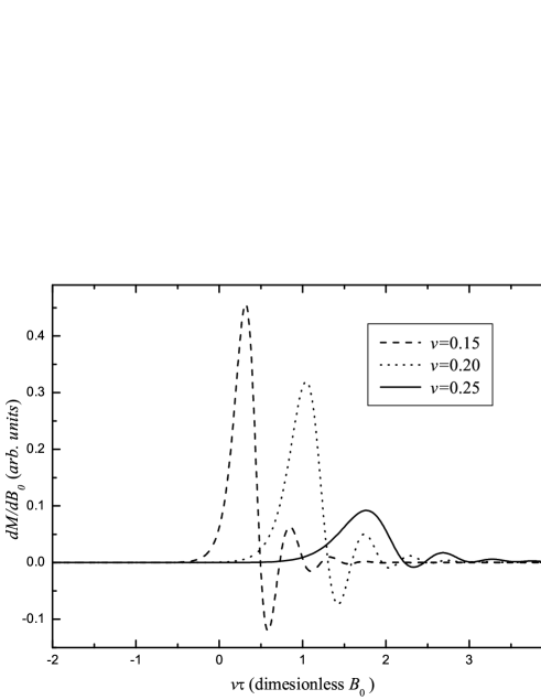
Figure 4: $dM/dB_{0}$ as a function of the dimensionless external magnetic field for different sweep rates. $\gamma=0.1,$ $\kappa=1$ and the dynamics is governed by Eqs. (25,26,27).

An important experimental result is that the position of the peaks in $dM/dB_{0}$ corresponding to the radiation process does depend on the external field sweep rate $v$. In our model this is related to the time spent by the sample around the resonance. For a slowly changing $B_{0}$, the dynamics is similar to the case of constant detuning, where an analytical solution is known, while increasing the value of $v$, an appropriate numerical solution of the dynamics is needed. In the case of superradiance, Fig. 4 shows $dM/dB_{0}$ as a function of $v\tau$, i.e., the dimensionless external field $B_{0}$. As we can see, for larger values of the sweep rate $v$, the height of the emission peak decreases and its position is shifted towards higher field values. The shift is in agreement with the experimental findings, while as a consequence of the coherent interaction, $dM/dB_{0}$ exhibits oscillations with sign changes.

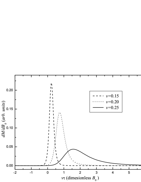
Figure 5: $dM/dB_{0}$ as a function of the dimensionless external magnetic field for different sweep rates. $\gamma=1,$ $\kappa=0.1$ but in contrast with Fig. 4, the rate equations (32) have been used to calculate the time evolution.

If we assume that the maser effect is responsible for the radiation and use the rate equations (32) to calculate the dynamics of the system, somewhat different results are obtained. As Fig. 5 shows, $dM/dB_{0}$ accompanied with maser radiation, scales similarly with $v$ as in the case of weak dephasing: larger sweep rates correspond to peaks at higher $B_{0}$ fields, thus taking the cavity effects into account, this scaling property is not characteristic for SR. However, the oscillations seen in the superradiant case are absent in Fig. 5.

We shall analyze now from the point of view of transversal relaxation if the observed radiation could be superradiance. The reduction procedure summarized in Sec. II allows us to calculate the matrix element $|s|$ and thus the characteristic time (22) of the emission process for any transition. As the experimentally observed radiation peaks were around $1.4$ T, we focus on this value of the external magnetic field. The level structure of the Hamiltonian (1) provides the resonant transition frequency for a given transition $m\rightarrow m^{\prime}$, as well as the population of the upper level according to the Boltzmann factor. In this way we can calculate $T_{0}$ for any transition as a function of the temperature of the sample. As for SR to occur the dephasing rate $\gamma=T_{0}/T_{2}$ must be small, so we should look for the transition with the minimal value of $T_{0}$. We found that below approx. $0.8$ K the transition $m=-10\rightarrow m^{\prime}=8$ provides the shortest $T_{0}$, while above this temperature the transition from $m=-6$ to $m^{\prime}=4$ yields the minimal characteristic time. As Fig. 6 shows, for low temperatures, i.e., ground state tunneling, the minimal $T_{0}$ is of the order of seconds. This is a consequence of the very small coupling coefficient $s$, corresponding to this transition. For higher temperatures when the transition $m=-6\rightarrow m^{\prime}=4$ provides the shortest characteristic time, $T_{0}$ significantly decreases as a function of temperature. This is a consequence of the relation $T_{0}\propto 1/(|s|\sqrt{N_{0}})$ (see Eq. (22)), where $N_{0}$ is temperature dependent. That is, above $0.8$ K, the most favorable conditions for superradiance might be realized in the case of the transition $m=-6\rightarrow m^{\prime}=4,$ with a still strong temperature dependence of $T_{0}$.

However, the energy emitted during a transition process is not necessarily the highest for the lowest $T_{0}$. In fact, the population of the $m=-6$ level – which determines the maximum number of the active molecules – is not large enough to explain the magnitude of the emitted energy observed in a recent experiment. Ref. [Hernandez-Minguez et al., 2005] reports on radiative bursts of duration of a few milliseconds, where (at 2 K) the total energy emitted by the sample was detected to be around $3$ nJ. Using the parameters of the experiment,Hernandez-Minguez et al. (2005) we investigated all the possible transitions and found the best agreement with the experimental data for the transition $m=-8\rightarrow m^{\prime}=6$, giving a value of $T_{0}$ in the ms range and a total emitted energy to be around 1.5 nJ. (Note that for initial states below $m=-8$ the time scale of the process turns out to be too long, while for $m>-8$ the number of active molecules is too small.) Thus our model predicts that the process having the most important role in producing the observed radiation is the transition $m=-8\rightarrow m^{\prime}=6.$

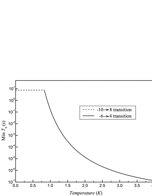
Figure 6: The minimal value (over the possible transitions) of $T_{0}$ given by Eq. (22) at $B_{0}=1.4$ T, where microwave emission from the sample has been detected. The minimum at low temperatures corresponds to the transition $m=-10\rightarrow m^{\prime}=8$, while above approx. $0.8$ K $m=-6\rightarrow m^{\prime}=4$ provides the shortest $T_{0}.$

As we have seen, the character of the emission depends on the ratio $\gamma=T_{0}/T_{2},$ where $T_{2}$ is decreasing with increasing temperature. According to Fig. 6, even for the shortest possible $T_{0}$ and relatively weak dephasing, with $T_{2}$ around $10^{-5}$–$10^{-6}$ s (Ref. [Leuenberger and Loss, 1999]), we have $\gamma>1$ at $2$ K. The millisecond time scale obtained here and observed also in the experiments is clearly longer than the relaxation time $T_{2}$. Thus – unless a yet unknown effect decreases the disturbance caused by phase relaxation – the process responsible for the experimentally observedTejada et al. (2004) bursts of radiation seems to be rather a maser effect than superradiance.

The fact that no emission was seen for external fields lower than 1.4 T (where there can be a resonance as well) can be explained by the strength of the coupling to the transversal mode: $|s|$ is generally at least an order of magnitude larger for the possibly relevant transitions at $1.4$ T than at previous resonances. However, in a good resonator – like the Fabry-Perot mirrors in Ref. [Tejada et al., 2003] – one may expect that several resonances have observable consequences, radiation and – as it has been detected – enhanced magnetic relaxation rates. Additionally, we note that at high sweep ratesVanacken et al. (2004) the system passes not only a single cavity resonance during the emission process, and consecutive resonances can broaden the peaks in the $dM/dB_{0}(B_{0})$ plots.

V Summary and Conclusions

In this paper we developed a model for the interaction of a crystal of molecular magnets with the magnetic field of a surrounding cavity. The sample itself generates this transversal field $B$, while it also acts back on the molecules. The most important point of our treatment is that the cavity mode with fixed frequency $\Omega$ comes to resonance with a magnetic transition at a given value of the external longitudinal magnetic field. Around this resonance the interaction of the molecules with the mode significantly increases leading to an observable burst of electromagnetic radiation as well as a change in the magnetization of the sample. Our model can describe different mechanisms of this radiation, in fact, there is a continuous transition from superradiance to maser-like effects. The crucial parameter here is the ratio of two time scales, the characteristic time of the process and the dephasing time $\gamma=T_{0}/T_{2}$. For small values of $\gamma$ the time evolution of the molecules is coherent allowing for the strong collective effect of superradiance in a cavity. In the case of strong dephasing, the sample still can emit electromagnetic radiation, but now the coherence of the molecules plays no role, the maser rate equations with time dependent detuning can describe the process. For moderate values of $\gamma$ we have a transition between the two processes. By calculating the intensity of the emitted radiation we have shown that with increasing the sweep rate of the external magnetic field, the emission peaks are shifted towards higher field values in accordance with the experimental results. This statement holds for both emission mechanisms, but the detailed functional dependencies are different for SR and maser emission.

Based on realistic approximations for $T_{0}$ and $T_{2}$, the process responsible for the experimentally observed bursts of electromagnetic radiation is most probably not superradiance, but rather a maser effect. The comparison of time resolved experiments on the emitted radiation with our theoretical results would provide the necessary information in order to settle this question. We expect that at very low temperatures, when spin-phonon relaxation is weaker, the collective features of the radiation may become dominant. While this is an interesting problem on its own, it is expected that the analysis of the radiated field can yield additional information on the process of quantum tunneling, as well as on the detailed properties of the interaction of these crystals and the field.