Matter wave pulses characteristics

Abstract

We study the properties of quantum single-particle wave pulses created by sharp-edged or apodized shutters with single or periodic openings. In particular, we examine the visibility of diffraction fringes depending on evolution time and temperature; the purity of the state depending on the opening-time window; the accuracy of a simplified description which uses “source” boundary conditions instead of solving an initial value problem; and the effects of apodization on the energy width.

I Introduction

Diffraction in time was discussed first by Moshinsky Moshinsky (1952). The hallmark of this phenomenon consists in temporal oscillations, deviating from the classical regime, of Schrödinger, matter waves released in one or several pulses from a preparation region in which they are initially confined. The original setting consisted of a sudden opening of a shutter to release a semi-infinite beam, and provided a quantum, temporal analogue of spatial Fresnel-diffraction by a sharp edge Moshinsky (1952); later more compicated shutter windows, initial confinements, and time-slit combinations have been considered Kleber , in particular two temporal slits and the corresponding interferences. Experimental observations have been carried out with ultracold neutrons Hils et al. (1998) and with ultracold atoms SSDD95 ; ASDS96 ; Szriftgiser et al. (1996). Recently, it has also been observed for electrons in a double temporal slit experiment Lindner et al. (2005). The “shutter problem” has indeed important applications, as it is the modelization of turning on and off a beam of atoms as done e.g. in integrated atom-optical circuits or a planar atom waveguide Schneble et al. (2003), and may allow us to translate the principles of spatial diffractive light optics to the time domain for matter waves BAKSZ98 . Besides, it provides a time-energy uncertainty relation Moshinsky (1976); Busch02 which has been verified experimentally for atomic waves, by realizing a Young interferometer with temporal slits SSDD95 ; ASDS96 ; Szriftgiser et al. (1996). The Moshinsky shutter has also been discussed with the Wigner function and tomographic probabilities Mánko et al. (1999), for relativistic equations Moshinsky (1952); GRV99 ; DMRGV , with dissipation Moshinsky et al. (2001); DMR04 , in relation to Feynman paths GVY03 , or for time dependent barriers SK88 , including the time dependence of states initially confined in a box when the walls are suddenly removed Gerasimov and Kazarnovskii (1976); Godoy02 . With adequate interaction potentials added to the model, it has been used to study and characterize transient dynamics of tunnelling matter waves Stevens ; TKF87 ; JJ89 ; Brouard and Muga (1996); GR97 ; GV01 ; GVDM02 ; DMRGV , and the transient response to abrupt changes of the interaction potential in semiconductor structures and quantum dots DCM02 ; AP .

Within the source boundary approximation, in which the form of the wave is imposed for all times at a source point or surface, many works have been carried out within the field of neutron interferometry Gahler et al. (1984); Felber et al. (1984), considering also a triangular aperture functions Felber et al. (1990), atom-wave diffraction Brukner et al. (1997), tunnelling dynamics Stevens ; Ranfa90 ; Ranfa91 ; Mor92 ; Büttiker and Thomas (1998); Muga and Büttiker (2000); DMRGV , and absorbing media, in which an ultrafast peak-propagation phenomenon has been recently described DMR04 .

The importance of pulse formation is nowadays enhanced due to the possibilities to control the aperture function of optical-shutters in atom optics, and to the development of atom lasers. For such devices some of the first mechanisms proposed explicitly implied periodically switching off and on the cavity mirrors, that is, the confining potential of the lasing mode. As an outcome, a pulsed atom laser is obtained. Much effort has been devoted to design a continuous atom laser, whose principle has been demonstrated using Raman transitions Moy et al. (1997); H99 . With this output coupling mechanism, an atom initially trapped suffers a transition to a nontrapped state, receiving a momentum kick during the process due to the photon emission. These transitions can be mapped to the pulse formation, so that the “continuous” nature of the laser arises as a consequence of the overlap of such pulses. There is in summary a strong motivation for a thorough understanding of matter-wave pulse creation, even at an elementary single-particle level.

In this paper we aim to describe the characteristics of one-dimensional, matter-wave pulses within the approximation in which interatomic interactions can be neglected, as it is usually the case in standard low-pressure atomic beams. This will be useful as a reference and first step to consider the interacting case later on. While the most idealized pulses have been studied in several works since the seminal paper of Moshinsky Moshinsky (1952), some aspects of realistic pulse production have not been examined with enough detail yet, such as the effects of statistical mixing in the preparation beam, or the fact that optical shutters do not have absolutely sharp edges, and could be taylored for designing the pulse features. Other main objective of the paper is to compare two ways to model boundary conditions: as a standard initial value problem where the wave is specified in the preparation region at time $t=0$, or according to the “source approach” in which the wave function is given for all times at the source point.

The organization of the papers is as follows: In Sec. II we review the Moshinsky shutter, whose main feature -diffraction in time- is quantified by means of the fringe visibility in Sec. III; Section IV deals with the evolution of finite pulses; In Sec. V the exact results are compared with the usual “source” approximation, and, finally, in Sec. VI the aperture function is modified for different types of apodization and the time-energy uncertainty product is evaluated. We also consider periodical shutter apertures and find analytical solutions for the wavefunction.

II Moshinsky shutter

In this section we review the “Moshinsky shutter” Moshinsky (1952, 1976) and discuss its physical interpretation. Consider a plane wave impinging from the left on a totally absorbing infinite potential barrier located at the origin (shutter) which is suddenly turned off at time zero. For $t=0$ one has the initial condition

$$\psi(x,t=0)=e^{ipx/\hbar}\Theta(-x),$$

where $\Theta$ is the step function, whereas for $t>0$ the wavefunction can be written using the free-particle Green’s function,

$$\psi(x,t) = \int_{-\infty}^{0}dx^{\prime}{\cal{G}}_{0}(x,t;x^{\prime},0)\psi(x,0)$$ (1)

$$= \frac{e^{\frac{imx^{2}}{2t\hbar}}}{2}\,w[-u(p,t)],$$

where

$${\cal{G}}_{0}(x,t;x^{\prime},0):=\sqrt{\frac{m}{2\pi i\hbar t}}\,e^{i\frac{m(x-x^{\prime})^{2}}{2\hbar t}},$$

$$u(p,t):=\frac{1+i}{2}\sqrt{\frac{t}{m\hbar}}\,\left(p-\frac{mx}{t}\right),$$ (2)

and

$$w(z):=e^{-z^{2}}{\rm{erfc}}(-iz)=\frac{1}{i\pi}\int_{\Gamma_{-}}du\frac{e^{-u^{2}}}{u-z},$$

is the “$w$” or “Faddeyeva” function Faddeyeva ; Abram . The contour $\Gamma_{-}$ goes from $-\infty$ to $\infty$ passing below the pole.

The associated “density” $|\psi(x,t)|^{2}$ exhibits diffraction in time, namely, a characteristic oscillation in time, and also in the space domain, see Fig. 1, in contrast with the simple step function for a spatially homogeneous ensemble of classical particles with momentum $p$ released at time $t=0$.

Figure 1: Diffraction in time seen in $P(\theta)$, Eq. (3), for an initial cut-off plane wave state.

Thanks to the relation between the $w$-function and Fresnel integrals Abram ,

$$C(\theta)+iS(\theta) = \frac{1+i}{2}\left[1-e^{i\pi\theta^{2}/2}w\left(\frac{1+i}{2}\pi^{1/2}\theta\right)\right],$$

$$\theta = \left(\frac{t}{m\hbar\pi}\right)^{\!\!\!1/2}\!\!\!(p-mx/t)=\frac{1-i}{\pi^{1/2}}u(p,t),$$

the solution may also be rewritten as

$$|\psi(x,t)|^{2}=P(\theta)=\frac{1}{2}\left\{\left[S(\theta)+\frac{1}{2}\right]^{2}+\left[C(\theta)+\frac{1}{2}\right]^{2}\right\},$$ (3)

and therefore be mapped onto the Cornu espiral, which is plotted in Fig. 2.

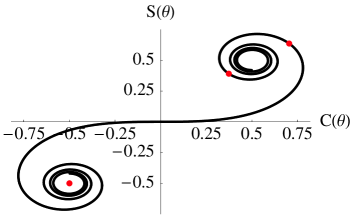
Figure 2: Cornu espiral. The points associated with the maximum and minimum of the largest fringe are plotted. They correspond to a maximum and a minimum of the distance to $(-1/2,-1/2)$.

The “density” can then be read as half the distance from the point $(-1/2,-1/2)$ to any other point of the spiral; and the origin corresponds to the classical particle with momentum $p$ released at time $t=0$ from the shutter position.

Suppose now that the shutter is closed suddenly at time $\tau$. The integrated “density” $N_{+}(\tau):=\int_{0}^{\infty}dx\,|\psi(x,\tau)|^{2}$ grows continuously with $\tau$ and may reach arbitrarily large values, obviously greater than one. Moreover, $|\psi(x,t)|^{2}$ is dimensionless, so $N_{+}$ cannot be taken as a probability in any case. This poses the question of physically interpreting the mathematical results. Clearly we face analogous problems to interpret a plane wave or stationary scattering states, which are not in Hilbert space. The solution is then found similarly, by assuming that $\psi(x,t)$, except for a normalization factor, is just a component of a normalizable state in Hilbert space, to be determined by the experimental preparation setup. A consistent interpretation for several -noninteracting- particles requires the appropriate quantum symmetrization Stevens84 , which will be treated elsewehere. In the present paper we shall limit ourselves to the simplest case an consider only one-particle states.

For a shutter with a non-zero reflectivity, the cut-off plane wave of opposite momentum has to be taken into account, so the initial state takes the form

$$\psi^{(\mathcal{R})}_{p}(x,t=0):=(e^{ip/\hbar x}+\mathcal{R}e^{-ip/\hbar x})\Theta(-x).$$ (4)

The cases $\mathcal{R}=\{1,0,-1\}$ turn out to be the most relevant. We will refer to $\mathcal{R}=-1$ as sine initial conditions, which arise when the shutter is totally reflective; and to $\mathcal{R}=1$ as cosine initial conditions. This last case may seem to be hard to implement but, surprisingly, it is related to the usual source boundary condition,

$$\psi_{p}^{s}(x=0,t)=e^{-i\omega t}\Theta(t),\;\;\psi_{p}^{s}(x>0,t\leq 0)=0,$$ (5)

where $\omega=p^{2}/(2m\hbar)$, and is more tractable mathematically than the sine case. As we shall see, $\psi^{s}_{p}(x,t)=\psi_{p}^{(1)}(x,t)$.

III Visibility of main diffraction fringe

Let us examine first the time evolution from a cut-off plane wave initial condition, i.e., $\mathcal{R}=0$, as in Eqs. (1) and (3). The motion of points of constant “density” is obtained by imposing a constant value of $\theta$, according to Eq. (3). In particular, for the maximum and nearby minimum, see Fig. 2,

$$x_{max}(t) = pt/m-\sqrt{\frac{\pi\hbar t}{m}}\theta_{max},$$

$$x_{min}(t) = pt/m-\sqrt{\frac{\pi\hbar t}{m}}\theta_{min},$$

where $\theta_{max}=1.217$ and $\theta_{min}=1.872$ are universal for $\mathcal{R}=0$. Since the probability is exclusively $\theta$-dependent, see Eq. (3), $P_{max}=1.370$, and $P_{min}=0.778$, independently of time, mass or momentum, and therefore the fringe visibility, defined as

$$\mathcal{V}(T)=\frac{P_{1^{st}max}-P_{1^{st}min}}{P_{1^{st}max}+P_{1^{st}min}},$$

is concluded to be universal (equal to 0.276 for $\mathcal{R}=0$), and of course time-independent.

Other important fringe feature is the width of the main peak. It can be computed from the intersection with the classical probability density (for a cut-off beam of particles released at time $0$ with momentum $p$) Moshinsky (1952, 1976),

$$\Delta x\simeq 0.85\left(\frac{\pi\hbar t}{m}\right)^{1/2}.$$

Next, we consider an initial state given by a statistical mixture,

$$\rho(t=0):=\int dpf(p)|\psi_{p}^{(\mathcal{R})}(t=0)\rangle\langle\psi_{p}^{(\mathcal{R})}(t=0)|,$$ (6)

and focus our attention on the effect of temperature and evolution time on the diffraction pattern. Let us assume, by integrating out the y,z-degrees of freedom of a Maxwell-Boltzmann momentum distribution Metcalf (1999), that the Gaussian momentum probability density

$$f_{MB}(p)=\frac{1}{\sqrt{2\pi mk_{B}T}}\;e^{-\frac{(p-p_{c})^{2}}{2mk_{B}T}},$$ (7)

holds for the momentum in $x$ direction. The introduction of a non-zero mean average momentum $p_{c}$ implies that the atomic ensemble, say in a magneto-optical trap, is launched along the $x$-axis with a velocity $p_{c}/m$. This is realized, for example, in the “moving molasses technique” Salomon within an atomic fountain clock. We shall generally assume that the contribution of negative $p$ in Eq. (7) is negligible.

Figure 3 shows the effect of the temperature on the visibility of the main diffraction fringe for statistical mixtures weighted by the distribution of Eq. (7), with $\mathcal{R}=\{0,\pm 1\}$.

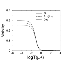
Figure 3: Visibility as a function of temperature and the reflectivity of the shutter for a beam of Argon with the distribution in Eq. (7). $p_{c}/m=10$ cm/s, $t=20\,\mu$s.

It is clear that the diffraction peaks are more visible for sine conditions than for the isolated cut-off plane wave and cosine conditions, the difference being more noticeable at small temperatures. As expected, there is a suppression of the diffraction pattern when the temperature increases. A possible criterion for this suppression is a small value of the ratio, $\alpha$, between the width of the fringe $\Delta x$ and the separation $\Delta x_{cl}$ of the classical arrival points corresponding to fast and slow components of the statistical mixture, namely,

$$\alpha:=\frac{\Delta x}{\Delta x_{cl}}=\frac{0.85}{\Delta p}\sqrt{\frac{m\pi\hbar}{t}}.$$

For the Gaussian distribution, Eq. (7), one can choose $\Delta p$ as the full width at half maximum (FWHM), that is, $2\sqrt{2ln2mk_{B}T}$, so that

$$\alpha=0.36\sqrt{\frac{\pi\hbar}{K_{B}Tt}}.$$

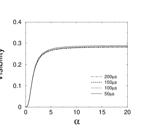
Figure 4: Visibility as a function of the $\alpha$-parameter for an Argon atom with a velocity $p_{c}/m=10$ cm/s. Each curve is computed by varying the temperature for a given opening time. $\mathcal{R}=-1$.

According to Fig. 4, the visibility grows with $\alpha$ for small values and saturates for large $\alpha$, i.e. for small times and/or temperatures.

Moreover, if instead of Eq. (7), the momentum distribution of an effusive atomic beam is used Ramsey ; Metcalf (1999),

$$f_{beam}(p)=\frac{p^{3}}{2(mk_{B}T)^{2}}\,e^{-\frac{p^{2}}{2mk_{B}T}}\Theta(p),$$ (8)

then $\langle p\rangle=\sqrt{9\pi mk_{B}T/8}$, and the upshot is a complete supression of the diffraction in time phenomena for all times and temperatures. This fact points out the relevant role played by the momentum distribution, that is, by the experimental preparation setup being considered.

Summing it up, the fringe visibility, at variance with the pure state case, becomes time-dependent for mixed states. The characteristic oscillations of diffraction in time tend to be washed out with the observation time after opening the shutter, and also by increasing the temperature, or for the momentum distribution of an effusive beam.

IV Evolution of a finite pulse

In this section we focus on the formation and evolution of a matter-wave, single-particle pulse. Suppose that the shutter is opened at the instant $t=0$ and closed at the instant $\tau$. We will refer to the duration $\tau$ as the “opening time”. It is, in other words, the width of the the time slit. The notation $\psi^{(\mathcal{R})}_{p_{0},\tau}(t)$ will denote the state formed in that manner, at time $t\geq\tau$, from the initial state of Eq. (4) with main momentum $p_{0}$.

For an initially pure state the time evolution of the pulse can be written in terms of the inner products with the eigenstates of the free hamiltonian which vanish at the origin,

$$\langle x|\phi_{E}\rangle=\sqrt{\frac{2m\hbar}{\pi p}}\sin{(px/\hbar)},\;\;\;E=p^{2}/(2m).$$

They obey orthonormality and completeness relations,

$$\langle\phi_{E^{\prime}}|\phi_{E}\rangle=\delta(E-E^{\prime}),\;\;\\ \int_{0}^{\infty}dE\,|\phi_{E}\rangle\langle\phi_{E}|=\openone.$$

As shown by Moshinsky Moshinsky (1976), the overlap between these eigenstates and the state that results from a state formed after an opening time $\tau$ with $\mathcal{R}=0$ is

$$\langle\phi_{E}|\psi_{p_{0},\tau}^{(0)}(t=\tau)\rangle=\sqrt{\frac{mp\hbar}{2\pi}}$$

$$\times \Bigg{\{}\!\frac{w[-u_{0}(p_{0},\tau)]}{p^{2}-p_{0}^{2}}\!-\!\frac{w[-u_{0}(p,\tau)]}{2p(p-p_{0})}\!-\!\frac{w[-u_{0}(-p,\tau)]}{2p(p+p_{0})}\Bigg{\}},$$

where

$$u_{0}(p,\tau):=\frac{1+i}{2}\sqrt{\frac{\tau}{m\hbar}}\,p,$$

to be compared with Eq. (2). ($u_{0}(p,\tau)$ is a particular case of $u(p,\tau)$ in which $x=0$.) The overlaps for the cases $\mathcal{R}=\pm 1$ are obtained easily from Eq. (IV).

Writing the final time of observation as $t=\tau+\Delta t$, the evolved pulse can then be calculated as

$$\psi^{(\mathcal{R})}_{p_{0},\tau}(x,t)=\int_{0}^{\infty}dE\,e^{-iE\Delta t/\hbar}\langle x|\phi_{E}\rangle\langle\phi_{E}|\psi^{(\mathcal{R})}_{p_{0},\tau}(t=\tau)\rangle.$$ (10)

This expression is not well-behaved numerically, but such a problem can be swiftly solved by modifying the contour of integration in the complex $p$-plane, since several terms can be written as $w$-functions (see the Appendices A and B for details), and for the rest we gain an integrand with Gaussian decay. Explicitly, for $\mathcal{R}=-1$,

$$\psi^{(-1)}_{p_{0},\tau}(x,t)=\frac{e^{\frac{imx^{2}}{2t\hbar}}}{2}\,\left\{[w[-u(p_{0},t)]+w[-u(-p_{0},t)]\right\}$$ (11)

$$- \frac{e^{-i\frac{p_{0}^{2}\tau}{2m\hbar}}-w[u_{0}(p_{0},\tau)]}{2}e^{\frac{imx^{2}}{2\Delta t\hbar}}$$

$$\times \left\{w[-u(p_{0},\Delta t)]+w[-u(-p_{0},\Delta t)]\right\}$$

$$\!-\! \!\frac{i}{2\pi}\int_{\Gamma_{+}}\!\!\!dp\,e^{-i\frac{p^{2}\tau}{2m\hbar}+ipx/\hbar}$$

$$\times \left\{\frac{w[u_{0}(-p,\tau)]}{p+p_{0}}+\frac{w[u_{0}(p,\tau)]}{p-p_{0}}\right\},$$

where the contour passes above the poles. This result is so far exact. The integral term, $\mathcal{Y}$, can be rewritten by integrating in the $u$ variable,

$$\mathcal{Y} = -\frac{ie^{\frac{imx^{2}}{2\Delta t\hbar}}}{2\pi}\int_{\Gamma_{u}}du\,{e^{-u^{2}}}$$ (12)

$$\times \left[\frac{w(\sqrt{\frac{\tau}{\Delta t}}u+v)}{u-u(p_{0},t)}+\frac{w(-\sqrt{\frac{\tau}{\Delta t}}u-v)}{u-u(-p_{0},t)}\right],$$

see the Appendix A, with

$$v=\frac{1+i}{2}\sqrt{\frac{\tau}{m\hbar}}\frac{mx}{\Delta t}.$$

A way of dealing with this kind of integral to excellent accuracy was discussed by Brouard and one the authors in Brouard and Muga (1996). It consists in extracting the singularities of the integrand, which we shall denote as $g(u)$, in the following way

$$g(u)=\sum_{i}\frac{A_{i}}{u-u_{i}}+h(u).$$

$A_{i}$ is the residue of $g(u)$ at the pole $u_{i}$ and $h(u)$ is an entire function which admits a power series expansion convergent in the whole $u$-plane,

$$\int_{-\infty}^{\infty}h(u)e^{-u^{2}}du$$

$$= \sqrt{\pi}\left[h(u=0)+\sum_{n=1}^{\infty}\frac{(2n-1)!!}{2^{n}(2n)!}\,h^{(2n)}(u=0)\right].$$

Retaining just the first term of the previous expansion leads to

$$\int_{\Gamma_{u}}du\,g(u)\simeq\sum_{i}A_{i}\left[-i\pi w(-u_{i})+\frac{\sqrt{\pi}}{u_{i}}\right]+\sqrt{\pi}g(u=0).$$

In particular,

$$\mathcal{Y} \simeq \!-\frac{e^{\frac{imx^{2}}{2\Delta t\hbar}}}{2}\left\{w[u_{0}(p_{0},\tau)]w[-u(p_{0},\Delta t)]\right.$$ (13)

$$+ \!\left.w[-u_{0}(p_{0},\tau)]w[-u(-p_{0},\Delta t)]\right\}$$

$$\!+\! \!\!\frac{ie^{\frac{imx^{2}}{2\Delta t\hbar}}}{2\sqrt{\pi}}\!\left\{\!\frac{w(v)\!-\!w[u_{0}(p_{0},\tau)]}{u(p_{0},\Delta t)}\right.$$

$$+ \left.\frac{w(-v)\!-\!w[-u_{0}(p_{0},\tau)]}{u(-p_{0},\Delta t)}\!\right\}\!,$$

which we shall use later on in Sec. V to compare the initial value problem and source approaches.

IV.1 Purity of the chopped state: coherence creation from incoherent mixtures by using small opening times

It is possible to “create coherence” from statistical mixtures, simply by means of small opening times. This was seen experimentally with cold atoms by Dalibard and coworkers Szriftgiser et al. (1996). To quantify this effect we use the purity, defined by

$$\mathcal{P}_{t}:=\rm{Tr}\rho_{N,\tau}^{2}(t),$$

where $\rho_{N,\tau}(t)$ is the normalized density operator at time $t$ for an opening time $\tau$. Our starting point is the unnormalized state

$$\rho_{\tau}(t):=\int dpf(p)|\psi^{(0)}_{p,\tau}(t)\rangle\langle\psi^{(0)}_{p,\tau}(t)|.$$ (14)

Thanks to the invariance under cyclic permutation of the trace and unitarity of the time evolution, the purity is invariant for $t\geq\tau$, so it can be calculated in particular at $t=\tau$,

$$\mathcal{P}_{\tau}=\frac{1}{N^{2}}\int\!\!\int dpdp^{\prime}f(p)f(p^{\prime})|\langle\psi^{(0)}_{p,\tau}|\psi^{(0)}_{p^{\prime},\tau}\rangle|^{2},$$

where $N$ is given by

$$N={\rm{Tr}}\rho_{\tau}=\int dpf(p)\langle\psi^{(0)}_{p,\tau}|\psi^{(0)}_{p,\tau}\rangle.$$

Considering the case of an effusive atomic beam, $f(p)=f_{beam}(p)$, Eq. (8), Fig. 5 shows that the purity ${\mathcal{P}}_{t}$ decreases as a function of the opening time and temperature. For short opening times a highly coherent state is created in spite of the mixed preparation state.

Figure 5: Variation of purity versus the opening time for different temperatures. An effusive beam of Argon atoms is considered, see Eq. (8). $\mathcal{R}=0$.

This result, in the limit $\tau\to 0$, may be understood as follows: As long as a (pure state) wavefunction vanishes in $x>0$ at time $t=0$, the wavefunction for $t>t^{\prime}>0$ can be written as Baute et al. (2001)

$$\psi(x,t)=\int_{0}^{t}dt^{\prime}K_{+}(t,x;t^{\prime},x^{\prime}=0)\psi(x^{\prime}=0,t^{\prime}),$$

where

$$K_{+}(t,x;t^{\prime},x^{\prime}=0) = \frac{\hbar}{mi}\frac{d}{dx}{\mathcal{G}}_{0}(x,t;0,t^{\prime})$$

$$= \left[\frac{m}{ih(t-t^{\prime})^{3}}\right]^{1/2}xe^{imx^{2}/2\hbar(t-t^{\prime})}.$$

By performing a Taylor series expansion in $t^{\prime}$ around $t^{\prime}=0$, one finds that

$$\psi(x,t)=tK_{+}(t,x;0,0)+\mathcal{O}(t^{2})$$

for $\psi(x=0,t^{\prime}=0)=1$. Since $\psi^{(0)}_{p,\tau}(x=0,t^{\prime}=0)=1$ for all $p$, then to first order all the momenta that form the preparation mixture give the same contribution, in other words, $|\psi_{p,\tau}(t)\rangle$ in Eq. (14) becomes independent of $p$, and thus the resulting state tends to be independent of the initial distribution $f(p)$, and totally coherent (pure) in the limit of small opening times. For the case of the Gaussian distribution in Eq. (7), the same qualitative behaviour (monotonic decay from $1$ in the same time scale) is observed.

V Comparison between “source” and “initial value problem” approaches

Golub and Gähler Gahler et al. (1984) tackled the diffraction in time problem in two dimensions using the Green’s function formalism, working within the Fraunhoffer limit, and imposed source boundary conditions. This approach was later thoroughly implemented for different combinations of time and space rectangular slits by Brukner and Zeilinger Brukner et al. (1997). Other works have used the simple source boundary conditions of Eq. (5) in one dimension, see Muga and Büttiker (2000), and references therein. In Baute et al. (2001) the relations between source boundary conditions and the initial value problem (IVP) were examined and equivalence conditions established.

In order to compare pulses formed by source or IVP approaches let us introduce the window function $\chi_{[0,\tau]}(t)=\Theta(t)\Theta(\tau-t)$ and impose the source boundary condition

$$\psi^{\,s}_{p_{0},\tau}(x=0,t)=e^{-i\omega_{0}t}\chi_{[0,\tau]}(t),$$ (15)

(the wave function is also assumed to vanish at $x>0$ for all $t\leq 0$) with Fourier transform

$$\widehat{\psi}^{\,s}_{p_{0},\tau}(x=0,\omega)=\frac{i}{\sqrt{2\pi}}\,\frac{1}{\omega-\omega_{0}}\big{[}1-e^{i(\omega-\omega_{0})\tau}\big{]}.$$

At a later time one finds, for $x>0$,

$$\psi^{\,s}_{p_{0},\tau}(x,t)=\frac{i}{2\pi}\int_{-\infty}^{\infty}d\omega\frac{e^{ipx/\hbar-i\omega t}}{\omega-\omega_{0}}\big{[}1-e^{i(\omega-\omega_{0})\tau}\big{]},$$

where ${\rm{Im}}p\geq 0$. This can be written in the complex $p$-plane by introducing the contour of integration $\Gamma_{+}$ which goes from $-\infty$ to $\infty$ passing above the poles,

$$\psi^{\,s}_{p_{0},\tau}(x,t)=\frac{i}{2\pi}\int_{\Gamma_{+}}dp\,2p\,\frac{e^{ipx/\hbar-i\frac{p^{2}t}{2m\hbar}}}{p^{2}-p_{0}^{2}}\big{[}1-e^{i(\omega-\omega_{0})\tau}\big{]}$$

$$= \frac{i}{2\pi}\int_{\Gamma_{+}}\!\!\!dp\,\left(\frac{1}{p+p_{0}}\!+\!\frac{1}{p-p_{0}}\right)e^{ipx/\hbar-i\frac{p^{2}t}{2m\hbar}}\big{[}1\!-\!e^{i(\omega-\omega_{0})\tau}\big{]}.$$

The integral can be carried out exactly using Appendix A,

$$\psi^{\,s}_{p_{0},\tau}(x,t)=\frac{e^{\frac{imx^{2}}{2t\hbar}}}{2}\,\{w[-u(p_{0},t)]+w[-u(-p_{0},t)]\}$$

$$\!\!-\frac{e^{-i\frac{p_{0}^{2}\tau}{2m\hbar}+\frac{imx^{2}}{2\Delta t\hbar}}}{2}\!\{w[-u(p_{0},\Delta t)]\!+\!w[-u(-p_{0},\Delta t)]\},$$

(16)

so the time evolution is straightforward and given by a difference of $w$-functions (in fact, expressing the window function as a difference of step functions $\chi_{[0,\tau]}=\Theta(t)-\Theta(t-\tau)$, the solution can be foreseen to be given by the difference of one source open at $t=0$ and a second one at a later time $t=\tau$, with the associated phase taken into account). The nice thing about this approach is that it allows a clear and intuitive interpretation of the different contributions to the total wavefunction, and it is easy to implement complicated combinations of time and space windows. The flip side is that deviations from the exact result of the initial value problem arise, specially for the back part of the wavefunction cut by the chopper, except in the case $\mathcal{R}=1$. Although the calculation is somewhat tedious -see Appendix C-, it can be proved that for cosine initial conditions, the wave function that results from a shutter opened between $0$ and $\tau$, $\psi_{p_{0},\tau}^{(1)}(x,t)$, is exactly equivalent to using source boundary conditions in that interval, i.e., to Eq. (V). The difference with the solution for the reflecting shutter ($\mathcal{R}=-1$) can be written as

$$\psi^{(-1)}_{p_{0},\tau}(x,t)-\psi^{(1)}_{p_{0},\tau}(x,t)\simeq\frac{e^{\frac{imx^{2}}{2\Delta t\hbar}}}{2}$$ (17)

$$\times \left\{w[u_{0}(p_{0},\tau)]-w[-u_{0}(p_{0},\tau)]\right\}w[-u(-p_{0},\Delta t)]$$

$$+ \!\frac{ie^{\frac{imx^{2}}{2\Delta t\hbar}}}{2\sqrt{\pi}}\left(\frac{w(v)-w[u_{0}(p_{0},\tau)]}{u(p_{0},\Delta t)}\right.$$

$$+ \left.\frac{w(-v)\!-\!w[-u_{0}(p_{0},\tau)]}{u(-p_{0},\Delta t)}\right),$$

where we have used Eqs. (11), (13) and (V). The overlap probability between pulses generated for different values of $\mathcal{R}$ and fixed $\tau$ and $p_{0}$,

$${\mathcal{O}}^{(\mathcal{R,R^{\prime}})}:=\frac{|\langle\psi^{(\mathcal{R})}|\psi^{(\mathcal{R}^{\prime})}\rangle|^{2}}{\langle\psi^{(\mathcal{R}^{\prime})}|\psi^{(\mathcal{R}^{\prime})}\rangle\langle\psi^{(\mathcal{R})}|\psi^{(\mathcal{R})}\rangle},$$ (18)

is independent of the evolution time $t$, and can be calculated exactly at $t=\tau$. It turns out to be a function of the adimensional phase $S/\hbar:=\tau p_{0}^{2}/(2m\hbar)$, see Fig. 6.

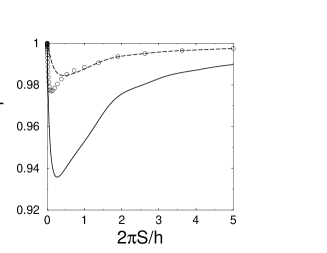
Figure 6: Overlap probability between the wavefunction of one Argon atom associated with sine and cosine initial conditions (continuous line), cut-off plane wave and sine conditions (circles), and cut-off plane wave and cosine conditions (dashed line), as a function of the phase $S/\hbar:=\tau p_{0}^{2}/(2m\hbar)$, see Eq. (18).

The overlaps tend to one as $\tau\to 0,\infty$. Remarkably, there is a lower bound which is 93.56% between sine and ${\emph{cosine}}-$source conditions. We may conclude that in general the result of using source boundary conditions is not at all a bad approximation to the solution of the initial value problem with reflecting or absorbing conditions, except when very accurate results are required.

VI Apodization of matter-wave pulses

Apodization is a technique long used in light optics to avoid the diffraction effect in several devices. Simply put, it consists in suppressing high frequency components by smoothing the aperture function (or “window” for short) of the pulse Fowles (1968). The price to pay is a slight broadening of the energy distribution. In this section such a technique is applied to matter wave pulses within the source approach. In particular, the case of a sine type aperture function can be analytically solved in terms of $w$-functions. Let us consider in Eq. (15), instead of the sudden, rectangular shape, a sine aperture function,

$$\chi_{[0,\tau]}(t)=\sin{(\Omega t)}\,\Theta(t)\,\Theta(\tau-t)$$ (19)

with $\tau=\pi\Omega^{-1}$. (Note that the “sine” aperture function has nothing to do with sine initial conditions.) Then, defining $\omega_{\pm}=\omega_{0}\pm\Omega$ and the corresponding momenta $p_{\pm}=\sqrt{2m\hbar\omega_{\pm}}$, with the branch cut taken along the negative imaginary axis of $\omega_{\pm}$, it is found that

$$\widehat{\psi}^{\,s}_{p_{0},\tau}(x=0,\omega)=\frac{1}{\sqrt{8\pi}}\,\left[\frac{1-e^{i(\omega-\omega_{-})\tau}}{\omega-\omega_{-}}-\frac{1-e^{i(\omega-\omega_{+})\tau}}{\omega-\omega_{+}}\right],$$

and the wavefunction is (we shall distinguish apodized pulses from the rectangular aperture pulses used so far by means of a tilde)

$$\!\widetilde{\psi}^{\,s}_{p_{0},\tau}(x,t)=\frac{-1}{2\pi}\!\sum_{\alpha=\pm}\alpha$$

$$\times \int_{-\infty}^{\infty}\!\!d\omega\,e^{-i\omega t+ipx/\hbar}\left[\frac{1-e^{i(\omega-\omega_{\alpha})\tau}}{\omega-\omega_{\alpha}}\right]$$

$$= \frac{-1}{2\pi}\!\sum_{\alpha=\pm}\!\alpha\!\int_{\Gamma_{+}}\!\!\!dp\,e^{ipx/\hbar}\Big{(}\!e^{-i\omega t}-e^{-i\omega\Delta t-i\omega_{\alpha}\tau}\!\Big{)}$$

$$\times \Bigg{(}\frac{1}{p\!+\!p_{\alpha}}\!+\!\frac{1}{p\!-\!p_{\alpha}}\!\Bigg{)}$$

$$= \!\frac{i}{2}\!\sum_{\alpha=\pm}\!\alpha\!\Bigg{(}\!e^{\frac{imx^{2}}{2t\hbar}}\left\{w[-u(p_{\alpha},t)]\!+\!w[-u(-p_{\alpha},t)]\right\}$$

$$- \!e^{-i\frac{p_{\alpha}^{2}\tau}{2m\hbar}\!+\!\frac{imx^{2}}{2\Delta t\hbar}}\!\left\{w[-u(p_{\alpha},\Delta t)]\!+\!w[-u(-p_{\alpha},\Delta t)]\right\}\Bigg{)}$$

$$= i\sum_{\alpha=\pm}\alpha\,\,\psi_{p_{\alpha},\tau}^{\,s}(x,t).$$

As it is clear from the last line, the apodization with the sine aperture function is equivalent to the introduction of two different momenta components whose values are related to the length of the pulse. Pictorically, a sine window pulse is equivalent to the coherent difference of two simultaneous pulses produced with sudden rectangular windows from speeded up and decelerated sources.

Similarly, other window functions, as the ones shown in Fig. 7 can be worked out.

Figure 7: Different aperture function studied. The smoothness at the edges increases in this order: rectangular (continuous line), sine (dotted line), Hanning (dashed) and Blackman (long dashed line).

For instance, the Hanning aperture function,

$$\chi_{[0,\tau]}(t) = \sin^{2}({\Omega t})\,\Theta(t)\,\Theta(\tau-t)$$ (20)

$$= \frac{1}{2}(1-\cos{2\Omega t})\,\Theta(t)\,\Theta(\tau-t),$$

after introducing $p_{\beta}=\sqrt{2m\hbar(\omega_{0}\pm 2\Omega)}$ with $\beta=\pm$, leads to

$$\widetilde{\psi}^{\,s}_{p_{0},\tau}(x,t)=\frac{1}{2}\left[\psi_{p_{0},\tau}^{\,s}(x,t)-\frac{1}{2}\sum_{\beta=\pm}\psi_{p_{\beta},\tau}^{\,s}(x,t)\right],$$

where the effect of the apodization is to subtract to the pulse with the source momentum two other matter-wave trains associated with $p_{\beta}$, all of them formed with rectangular aperture functions.

A related configuration wich can be solved analytically in terms of $w$-functions is the source apodized periodically to create successive pulses. This can be done extending Eq. (20) to all positive times. The result is

$$\widetilde{\psi}^{\,s}_{p_{0},\tau}(x,t)=\frac{e^{\frac{imx^{2}}{2t\hbar}}}{4}\left\{w[-u(p_{0},t)]+w[-u(-p_{0},t)]\right\}$$

$$- \frac{1}{8}\sum_{\beta=\pm}e^{\frac{imx^{2}}{2t\hbar}}\left\{w[-u(p_{\beta},t)]+w[-u(-p_{\beta},t)]\right\}.$$

Note again the intervention of three different momenta. A consequence is that the $w$-function for the fastest component will eventually separate spatially as a smoother -rather than pulsed- forerunner, see Fig. 8.

Figure 8: Front part of the probability density for the periodic Hanning function at $t=1.2$ ms, with an aperture time $\tau=10\mu$s. The circle, diamond and square mark respectively the classical position of the slow $(p_{-})$, original $(p_{0})$ and accelerated $(p_{+})$ components. $p_{0}/m=10$ cm/s.

Also suitable for suppression of the sidelobes is the so-called Blackman aperture function,

$$\chi_{[0,\tau]}(t)=0.42-0.5\cos(2\Omega t)+0.08\cos(4\Omega t).$$

Using the $p_{\beta}$ defined above and the momenta

$$p_{\gamma}=\sqrt{2m\hbar(\omega_{0}\pm 4\Omega)},\;\,$$

with $\beta,\gamma=\pm$, one can write the time evolved wavefuntion in terms of twenty $w$-functions,

$$\widetilde{\psi}_{p_{0},\tau}^{\,s}(x,t) = 0.42\psi^{\,s}_{{p_{0}},\tau}(x,t)-0.25\sum_{\beta=\pm}\psi^{\,s}_{{p_{\beta}},\tau}(x,t)$$

$$+ 0.04\sum_{\gamma=\pm}\psi^{\,s}_{{p_{\gamma}},\tau}(x,t),$$

so, once again, the smoothed shutter is related to a combination of different pulses from rectangular time slits.

The probability density for a single pulse and the details of the secondary diffraction peaks for four different aperture functions are illustated in Figs. 9 and 10, where all states are normalized to one. As expected, the smoother the time window function, the higher the suppression of the sidelobes. Note that the Blackman apodized pulse is slightly more advanced that the other ones due to the faster components induced by this particular apodization.

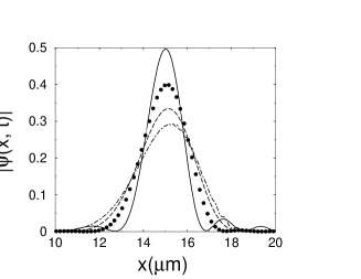
Figure 9: Probability density of a pulse of ultracold Argon atoms ($p_{0}/m=10$ cm/s), with $\tau=10\,\mu$s registered at $t=200\,\mu$s for different window functions: rectangular (continuous line), sine (dotted line), Hanning (dashed line) and Blackman (dot-dashed line).

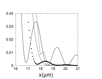
Figure 10: Detail of the sidelobes of the previous figure.

VI.1 Time-Energy uncertainty relation

A time energy uncertainty relation was discussed for the shutter problem by Moshinsky, who calculated the energy distribution of a particle after closing the shutter Moshinsky (1976). Using cosine conditions with energy $E$ and taking the overlap of the wavefunction with the free particle eigenstates which vanish at the origin, he calculated the energy distribution when the shutter was open a time $\tau$,

$$\wp(E,E^{\prime},\tau)=\mathcal{N}\sqrt{E^{\prime}}\,\frac{\sin^{2}[(E-E^{\prime})\tau/2\hbar]}{(E-E^{\prime})^{2}},$$

$\mathcal{N}$ being the normalization constant. Then it was concluded that, for some measure of the energy width Moshinsky (1976) (see Busch02 for a comprehensive review of time-energy uncertainty relation),

$$\Delta E\,\,\tau\,\simeq\,\hbar.$$

In fact, if one introduces the root of the variance $\sigma_{E}$ as the measure of energy spreading, $\Delta E=\sigma_{E}$, such an uncertainty relation cannot be established since $\sigma_{E}$ diverges. This is in consonace with the non-existence of the average displacement, $\langle x\rangle$, for sharply cut waves Marchewka and Schuss (1998). One can calculate also the energy distribution for the case of a sine-aperture function and source boundary conditions, Eq. (19), analytically. It turns out to be slightly broadened, but the variance is now well-defined as a consequence of the supression of high frequency sidelobes.

Alternatively, as done in Szriftgiser et al. (1996), the FWHM can be taken as the measure of energy spread. One observes that in both cases, sudden and smooth shutter, both measures of the spread decrease with the opening time. The uncertainty product is represented versus the opening time in Fig. 11.

Figure 11: Uncertainty product, $\Delta E\tau$, for a pulse of ultracold Argon atoms ($p_{0}/m=10$ cm/s): sine aperture function and $\Delta E=FWHM$ (solid line); sine aperture function and $\Delta E=\sigma_{E}$ (dotted line); rectangular aperture function with $\Delta E=FWHM$ (dashed line).

Note the two regimes, first a linear growth and then saturation, separated by the characteristic time required for a classical particle to travel a de Broglie wavelenght,

$$\top=\frac{hm}{p_{0}^{2}}.$$

VII Concluding remarks

Starting with a brief review of the Moshinsky shutter problem, we have examined several one-dimensional, matter-wave pulse characteristics such as the visibility of the diffraction-in-time fringes versus evolution time and temperature, or the creation of coherence by small aperture times. Moreover, a long standing missed comparison among several initial conditions used in previous works, which differed on the reflected components in the preparation region, has been carried out. We have studied several apodizations of the aperture function, and obtained analytical expressions for the time evolution of the corresponding pulses, also in the periodic case. The effects of apodization to suppress secondary diffraction peaks and in the energy width have been discussed.

The present work is the first step towards a more ambitious objective, namely, tayloring the pulses for particular needs, including the case in which interatomic interaction is important. Applications for laser atoms, in particular, will require in general to consider non-linear effects. Physically, optical shutters formed by effective potentials due to detuned lasers offer a unique oportunity, not available with mechanical shutters, to control the formation and subsequent behavior of the pulse.

Appendix A Integrals

Consider the following integral along a contour which goes from $-\infty$ to $\infty$ passing above the pole at $p_{0}$,

$$\mathcal{I}=\int_{\Gamma_{+}}dp\frac{e^{-iap^{2}+ibp}}{p-p_{0}},\;\;\;a>0.$$

The saddle point is at $p_{s}=b/2a$. By completing the square, one is lead to introduce the variable

$$u=u(p)=\frac{1+i}{\sqrt{2}}\left(\sqrt{a}p-\frac{b}{2\sqrt{a}}\right).$$

Deforming the contour to go along the steepest descent path from the saddle, which in the $u$-plane is at the origin,

$$\mathcal{I}=e^{i\frac{b^{2}}{4a}}\int_{\Gamma_{u}}du\frac{e^{-u^{2}}}{u-u(p_{0})},$$

If $\mathcal{C}_{0}$ denotes a counterclockwise circle around the pole $u(p_{0})$, then $\Gamma_{u}=(-\infty,\infty)\cup\mathcal{C}_{0}$ if the pole has been crossed ($Im(u)>0$) and the real line of $u$ otherwise. We can inmediatly recognize this integral as a Faddeyeva function since the following equalities hold thanks to Cauchy’s theorem,

$$\!\!\frac{1}{i\pi}\int_{\Gamma_{+}}du\frac{e^{-u^{2}}}{u-u(p_{0})}$$

$$= \frac{1}{i\pi}\int_{\Gamma_{-}}du\frac{e^{-u^{2}}}{u-u(p_{0})}-2e^{-[u(p_{0})]^{2}}$$

$$= w[u(p_{0})]-2e^{-[u(p_{0})]^{2}}=-w[-u(p_{0})],$$

where $\Gamma_{+}$ and $\Gamma_{-}$ go from $-\infty$ to $\infty$ passing above and below the pole, respectively. One concludes that

$$\mathcal{I}=-i\pi e^{i\frac{b^{2}}{4a}}w[-u(p_{0})].$$

Appendix B sine initial conditions

After opening the shutter and closing it at time $\tau$, the wavefunction for a reflecting shutter, ${\mathcal{R}}=-1$, is given by

$$\psi^{(-1)}_{p,\tau}(x,t)=\psi^{(0)}_{p,\tau}(x,t)-\psi^{(0)}_{-p,\tau}(x,t),$$

which is a difference of $w$-functions.

Since, using Eqs. (IV) and (10),

$$\psi^{(0)}_{p,\tau}(x,t)=\frac{1}{2\pi}\int_{-\infty}^{\infty}dp^{\prime}p^{\prime}\,e^{-i\frac{p^{\prime 2}\Delta t}{2m\hbar}}\sin(p^{\prime}x/\hbar)$$

$$\times \!\!\Bigg{\{}\frac{w[-u_{0}(p,\tau)]}{p^{\prime 2}-p^{2}}-\frac{w[-u_{0}(p^{\prime},\tau)]}{2p^{\prime}(p^{\prime}-p)}-\frac{w[-u_{0}(-p^{\prime},\tau)]}{2p^{\prime}(p^{\prime}+p)}\Bigg{\}},$$

the wavefunction can be written as

$$\psi^{(-1)}_{p,\tau}(x,t)=\frac{i}{8\pi}\int_{-\infty}^{\infty}dp^{\prime}e^{-i\frac{p^{\prime 2}\Delta t}{2m\hbar}}(e^{ip^{\prime}x/\hbar}-e^{-ip^{\prime}x/\hbar})$$

$$\times \!\!\Bigg{\{}\frac{w[u_{0}(p^{\prime},\tau)]\!-\!w[-u_{0}(p^{\prime},\tau)]\!-\!w[-u_{0}(p,\tau)]\!+\!w[u_{0}(p,\tau)]}{p^{\prime}+p}$$

$$+ \!\!\frac{w[-u_{0}(p^{\prime},\tau)]\!-\!w[u_{0}(p^{\prime},\tau)]\!-\!w[-u_{0}(p,\tau)]\!+\!w[u_{0}(p,\tau)]}{p^{\prime}-p}\Bigg{\}}.$$

Using the symmetry under $p^{\prime}\rightarrow-p^{\prime}$ the previous expression is simplified to

$$\langle x|\psi^{(-1)}_{p,\tau}(t)\rangle=\frac{i}{4\pi}\int_{-\infty}^{\infty}dp^{\prime}e^{-i\frac{p^{\prime 2}\Delta t}{2m\hbar}+ip^{\prime}x/\hbar}$$

$$\times \!\!\!\Bigg{\{}\frac{w[u_{0}(p^{\prime},\tau)]\!-\!w[-u_{0}(p^{\prime},\tau)]\!-\!w[-u_{0}(p,\tau)]\!+\!w[u_{0}(p,\tau)]}{p^{\prime}+p}$$

$$+ \!\!\frac{w[-u_{0}(p^{\prime},\tau)]\!-\!w[u_{0}(p^{\prime},\tau)]\!-\!w[-u_{0}(p,\tau)]\!+\!w[u_{0}(p,\tau)]}{p^{\prime}-p}\Bigg{\}},$$

where the relation

$$w(z)+w(-z)=2e^{-z^{2}}$$ (22)

can be applied leading to

$$\psi^{(-1)}_{p,\tau}(x,t) = \frac{-i}{2\pi}\int_{-\infty}^{\infty}dp^{\prime}e^{-i\frac{p^{\prime 2}\Delta t}{2m\hbar}+ip^{\prime}x/\hbar}$$ (23)

$$\times \bigg{\{}e^{-i\frac{p^{2}\tau}{2m\hbar}}-w[u_{0}(p,\tau)]-e^{-i\frac{p^{\prime 2}\tau}{2m\hbar}}\bigg{\}}$$

$$\times \left(\frac{1}{p^{\prime}+p}+\frac{1}{p^{\prime}-p}\right)+\mathcal{Y},$$

with

$$\mathcal{Y} = -\frac{i}{2\pi}\int_{-\infty}^{\infty}dp^{\prime}e^{-i\frac{p^{\prime 2}\Delta t}{2m\hbar}+ip^{\prime}x/\hbar}$$

$$\times \left\{\frac{w[u_{0}(p^{\prime},\tau)]}{p^{\prime}-p}+\frac{w[-u_{0}(p^{\prime},\tau)]}{p^{\prime}+p}\right\}.$$

The resulting integrals, but for the term $\mathcal{Y}$, are of the form solved in Appendix A. The final result is Eq. (11).

Appendix C cosine initial conditions

The solution to the Moshisnky shutter with cosine initial conditions, ${\mathcal{R}}=1$,

$$\psi_{p}^{(1)}(x,t)=\frac{e^{\frac{imx^{2}}{2t\hbar}}}{2}\,\{w[-u(p,t)]+w[-u(-p,t)]\},$$

is immediately computed from Eq. (1). The same result is obtained using the source boundary conditions of Eq. (5) and following the steps leading to Eq. (16).

In fact the same agreement can be extended to finite opening times $\tau$. The procedure to obtain $\psi_{p_{0},\tau}^{(1)}(x,t)$ is very much the same as for the sine case. Using

$$\psi^{(1)}_{p,\tau}(x,t)=\psi^{(0)}_{p,\tau}(x,t)+\psi^{(0)}_{-p,\tau}(x,t),$$

the expressions for the $\psi^{(0)}_{\pm p,\tau}(t)$ in Eq. (LABEL:psi0), the identity in Eq. (22), and $t=\tau+\Delta t$, one finds

$$\psi^{(1)}_{p,\tau}(x,t) = \frac{i}{4\pi}\int_{-\infty}^{\infty}dp^{\prime}\,\left(e^{-i\frac{p^{\prime 2}t}{2m\hbar}}-e^{-i\frac{p^{2}\tau}{2m\hbar}}e^{-i\frac{p^{\prime 2}\Delta t}{2m\hbar}}\right)$$

$$\times \left({e^{ip^{\prime}x/\hbar}-e^{-ip^{\prime}x/\hbar}}\right)\left(\frac{1}{p^{\prime}+p}+\frac{1}{p^{\prime}-p}\right).$$

Due to the symmetry under $p^{\prime}\rightarrow-p^{\prime}$ the term with $-e^{-ip^{\prime}x/\hbar}$ is equal to the one with $e^{ip^{\prime}x/\hbar}$ and the resulting integral can be carried out by completing the square and deforming the contour of integration in the complex $p$-plane as described in Appendix A, so new Faddeyeva functions can be identified. This leads to the same expression found in Eq. (V).

References

- Moshinsky (1952) M. Moshinsky, Phys. Rev. 88, 625 (1952).
- (2) M. Kleber, Phys. Rep. 236, 331 (1994).
- Hils et al. (1998) T. Hils, J. Felber, R. Gähler, W. Gläser, R. Golub, K. Habicht, and P. Wille, Phys. Rev. A 58, 4784 (1998).
- (4) A. Steane, P. Szriftgiser, P. Desbiolles, and J. Dalibard, Phys. Rev. Lett. 74, 4972 (1995).
- (5) M. Arndt, P. Szriftgiser, J. Dalibard, and A. M. Steane, Phys. Rev. A 53, 3369 (1996).
- Szriftgiser et al. (1996) P. Szriftgiser, D. Guéry-Odelin, M. Arndt, and J. Dalibard, Phys. Rev. Lett. 77, 4 (2003).
- Lindner et al. (2005) F. Lindner at al., eprint quant-ph/0503165.
- Schneble et al. (2003) D. Schneble, M. Hasuo, T. Anker, T. Pfau, and J. Mlynek, J. Opt. Soc. Am. B 20, 648 (2003).
- (9) S. Bernet, R. Abfalterer, C. Keller, J. Schmiedmayer, and A. Zelinger, J. Opt. Soc. Am. B 15, 2817 (1998).
- Moshinsky (1976) M. Moshinsky, Am. Jour. Phys. 44, 1037 (1976).
- (11) P. Busch, in Time in Quantum Mechanics, edited by J. G. Muga, R. Sala and I. Egusquiza (Springer, Berlin, 2002), Ch. 3.
- Mánko et al. (1999) V. Mánko, M. Moshinsky, and A. Sharma, Solid State Commun. 94, 979 (1999).
- (13) G. García-Calderón, A. Rubio, and J. Villavicencio, Phys. Rev. A 59, 1758 (1999).
- (14) F. Delgado, J. G. Muga, A. Ruschhaupt, G. García-Calderón, and J. Villavicencio, Phys. Rev. A 68, 032101 (2003).
- Moshinsky et al. (2001) M. Moshinsky, and D. Schuch, J. Phys. A 34, 4217 (2001).
- (16) F. Delgado, J. G. Muga, and A. Ruschhaupt, Phys. Rev. A 69, 022106 (2004).
- (17) G. García-Calderón, J. Villavicencio, and N. Yamada, Phys. Rev. A 67, 052106 (2003).
- (18) G. Scheitler and M. Kleber, Z. Phys. D 9, 267 (1988).
- Gerasimov and Kazarnovskii (1976) A.S. Gerasimov and M.V. Kazarnovskii, Sov. Phys. JETP 44, 892 (1976).
- (20) S. Godoy, Phys. Rev. A 65, 042111 (2002).
- Brouard and Muga (1996) S. Brouard and J. G. Muga, Phys. Rev. A 54, 3055 (1996).
- (22) G. García-Calderón and A. Rubio, Phys. Rev. A 55, 3361 (1997).
- (23) G. García-Calderón and J. Villavicencio, Phys. Rev. A 64, 012107 (2001).
- (24) G. García-Calderón, J. Villavicencio, F. Delgado, and J. G. Muga, Phys. Rev. A 66, 042119 (2002).
- (25) K. W. H. Stevens, Eur. J. Phys. 1, 98 (1980); J. Phys. C 16, 3649 (1983).
- (26) N. Teranishi, A. M. Kriman, and D. K. Ferry, Superlatt. Microstruct. 3, 509 (1987).
- (27) A. P. Jauho and M. Jonson Superlatt. Microstruct. 6, 303 (1989).
- (28) F. Delgado, H. Cruz, and J. G. Muga, J. Phys. A 35, 10377 (2002).
- (29) F. Delgado, J. G. Muga, D. G. Austing, and G. García-Calderón, J. Appl. Phys. 97, 013705 (2005).
- Gahler et al. (1984) R. Gähler and R. Golub, Z. Phys. B 56, 5 (1984).
- Felber et al. (1984) J. Felber, R. Gähler, and R. Golub, Physica B 151, 135 (1988).
- Felber et al. (1990) J. Felber, G. Müller, R. Gähler, and R. Golub, Physica B 162, 191 (1990).
- Brukner et al. (1997) C. Brukner and A. Zeilinger, Phys. Rev. A 56, 3804 (1997).
- (34) A. Ranfangi, D. Mugnai, P. Fabeni, and P. Pazzi, Phys. Scr. 42, 508 (1990).
- (35) A. Ranfangi, D. Mugnai, and A. Agresti, Phys. Lett. A 158, 161 (1991).
- (36) P. Moretti, Phys. Scripta 45, 18 (1992).
- Büttiker and Thomas (1998) M. Büttiker and H. Thomas, Superlatt. Microstruct. 23, 781 (1998).
- Muga and Büttiker (2000) J. G. Muga and M. Büttiker, Phys. Rev. A 62, 023808 (2000).
- Moy et al. (1997) G. M. Moy, J. J. Hope, and C. M. Savage, Phys. Rev. A 55, 3631 (1997).
- (40) E. W. Hagley, L. Deng, M. Kozuma, J. Wen, K. Helmerson, S. L. Rolston, and W. D. Phillips, Science 283, 1706 (1999).
- (41) V. N. Faddeyeva and N. M. Terentev, Mathematical Tables: Tables of the values of the function for complex argument (Pergamon, New York, 1961).
- (42) Handbook of Mathematical Functions, edited by M. Abramowitz and I. A. Stegun (Dover, New York, 1965).
- (43) K. W. H. Stevens, J. Phys. C: Solid State Phys. 17, 5735 (1984).
- Metcalf (1999) H. J. Metcalf and P. van der Straten, Laser cooling and trapping (Springer, New York, 1999).
- (45) N. F. Ramsey, Molecular Beams (Oxford, London, 1956).
- Baute et al. (2001) A.D. Baute, I.L. Egusquiza, and J.G. Muga, J. Phys. A 34, 4289 (2001).
- Fowles (1968) G. R. Fowles, Introduction to modern optics (Dover, New York, 1968).
- Marchewka and Schuss (1998) A. Marchewka and Z. Schuss, eprint quant-ph/0504105.
- (49) A. Clairon, Ph. Laurent, A. Nadir, M. Drewsen, D. Grison, B. Lounis, and C. Salomon, in Proceedings of 6th European Frequency and Time Forum, EFTF, 1992.