Trapping and coherent manipulation of a Rydberg atom on a microfabricated device: a proposal

Abstract

We propose to apply atom-chip techniques to the trapping of a single atom in a circular Rydberg state. The small size of microfabricated structures will allow for trap geometries with microwave cut-off frequencies high enough to inhibit the spontaneous emission of the Rydberg atom, paving the way to complete control of both external and internal degrees of freedom over very long times. Trapping is achieved using carefully designed electric fields, created by a simple pattern of electrodes. We show that it is possible to excite, and then trap, one and only one Rydberg atom from a cloud of ground state atoms confined on a magnetic atom chip, itself integrated with the Rydberg trap. Distinct internal states of the atom are simultaneously trapped, providing us with a two-level system extremely attractive for atom-surface and atom-atom interaction studies. We describe a method for reducing by three orders of magnitude dephasing due to Stark shifts, induced by the trapping field, of the internal transition frequency. This allows for, in combination with spin-echo techniques, maintenance of an internal coherence over times in the second range. This method operates via a controlled light shift rendering the two internal states’ Stark shifts almost identical. We thoroughly identify and account for sources of imperfection in order to verify at each step the realism of our proposal.

1 Introduction

In recent years we have witnessed convergence between many fields of physics previously considered disparate. This has been particularly true in the case of solid state and atomic physics. On one side, the possibility of designing nanometric devices and the understanding of quantum phenomena in devices such as Josephson junctions has allowed experimentalists to control the quantum coherence of semi- QI_SISPINYAMAMOTO05 or super-conducting QI_QUANTRONIUM02 ; QI_NAKAMURABOX02 systems, exactly as was done many years ago for atoms or molecules. On the other, atomic physicists have been able to produce Bose-Einstein condensates MX_CORNELLBEC95 and degenerate Fermi gases MX_FERMIJIN99 in quasi ideal situations, wonderful tools for probing many body theory and mesoscopic physics.

Atom-chip experiments SCHMIEDMAYERREVIEW_99 ; MX_HANSCHCHIP99 open the way to investigations at the frontier of these two fields. Aside from their relative ease of use and potential as atom interferometers, they provide an ideal environment in which atomic ensembles can be integrated with, and coupled to, devices on a microcircuit. Moreover, they allow for the study of atom-surface interactions with a completely new degree of control. Separately, experiments on circular Rydberg atoms have proven them extremely sensitive probes of electric and magnetic fields, both static and dynamic, making ideal tools for the investigation of numerous quantum phenomena, atom-surface interactions included. This remarkable sensitivity, in conjunction with their relative ease of detection, makes a single circular Rydberg atom an excellent probe of microwave field intensities ranging from one to a few tens of photons ENS_RMP . The coupling of a single such atom to a high Q superconducting microwave cavity has allowed our group to study, for example, the decoherence of mesoscopic ensembles of photons ENS_CAT and to realize elementary quantum logic operations ENS_GHZ . In these experiments, circular Rydberg atoms are excited from a thermal atomic beam (mean velocity 350 m/s) crossing a cryogenic setup in which the superconducting cavity is mounted. The use of thermal atoms intrinsically limits the maximum interaction time between the atom and the microwave field. Moreover, in order to reduce to a negligible level the proportion of unwanted events in which we have more than one circular Rydberg atom present at once in the cavity, we are forced to work with a very low rate of excitation towards the Rydberg levels. Aside from increasing dramatically the acquisition time, this lack of a deterministic atom source is an inconvenience from the point of view of quantum information processing.

The integrated trapping and manipulation of circular Rydberg atoms on a chip proposed here would lift these limitations. If we are to take advantage, however, of the longer interaction times achievable with such trapped Rydberg atoms, we must also combine in the same setup the capability for the extension of the natural lifetime and long term coherent manipulation. For short term manipulation over times of the order of the millisecond, this being much shorter than their lifetime in free space, one could simply excite the Rydberg atoms from an initial sample of cold trapped atoms and study them in free fall QI_GRANGIERRYD02 . In Ref. ENS_TRAPRYDBERG04 we proposed an electric trap able not only to store an individual circular Rydberg atom, but also to inhibit its spontaneous emission and maintain an internal coherence. In this paper we present in much more detail how we assess the trap’s performance, how to integrate it on a chip and how we simulate the different imperfections of the setup. We not only present the trap geometry of Ref. ENS_TRAPRYDBERG04 but also show that it is possible to extend the proposal to a smaller design where the atom is brought closer to the chip surface, a design therefore better adapted to atom-surface interaction studies. The principle of the trap, along with its implementations in realistic geometries, is discussed in Sec. 2. We show in Sec. 3 that the excitation of a sample of ground state atoms, initially trapped on a magnetic atom chip, can lead to the preparation of a single Rydberg atom, taking advantage of the dipole-blockade effect QI_LUKINDIPOLEBLOCKADE01 . As explained above, the maximum duration of an experiment with this atom is not limited by the storage time but by the lifetime of the circular Rydberg state. We discuss in Sec. 4 the efficiency of the spontaneous emission inhibition when we place our atom chip within a structure excluding the millimetre-wave decay channel. We show that the radiative lifetime could realistically be pushed into the second range. We present finally in Sec. 5 a technique taking advantage of a controlled light shift of the Rydberg levels allowing for the maintenance and control over a similar duration of the coherence of an atom in a superposition of two trapped states.

2 A microfabricated electrodynamic trap for Rydberg atoms

The large coupling of Rydberg atoms to static or time-varying fields presents us with numerous possible trapping techniques. It has been proposed, for example, to use powerful, far-detuned laser beams to create very tight traps for Rydberg states. These traps exploit the ponderomotive force TR_PONDEROMOTIVE00 experienced by the atom due to the fast oscillation of its valence electron in the laser field. It remains hard however to fulfill all the criteria allowing for coherent manipulation of Rydberg levels in any such trap. For instance, one can see that the very large laser power required by the ponderomotive trapping is hardly compatible with the cryogenic environment necessary to avoid blackbody radiation in the microwave domain ENS_RMP and the consequent destabilization of the Rydberg levels.

Another possible solution is to use d.c. magnetic fields and conventional atom-chip architectures. The magnetic moment of a Rydberg level (principal quantum number $n$) can be of the order of $n\mu_{B}$, where $\mu_{B}$ is the Bohr magneton. The same atom-chip wires could be used for the trapping of ground and Rydberg state atoms. One possible problem is that the Rydberg state might be affected by its interaction with still-trapped ground-state atoms in its vicinity. Moreover, the transition frequency between different Rydberg states is strongly perturbed by the Zeeman effect. We could not find a way to suppress the resulting random dephasing, in contrast to that due to the Stark effect, which can be partially compensated as explained in Sec. 5.

In the following we therefore use time-varying electric fields to trap the Rydberg atoms.

2.1 Circular Rydberg atoms in an electric field

We consider the case of Rydberg atoms in circular states. These have a large principal quantum number $n$, of the order of 50 in our discussion, along with maximal angular and magnetic quantum numbers ($l=|m|=n-1$). The atom therefore has both a large energy and a large angular momentum. The classical analog of the electron’s wavefunction is a Keplerian circular orbit around the nucleus. To be concrete we will consider ⁸⁷Rb atoms. To a very good approximation one can neglect the fine structure corrections to the circular levels’ energies and assume that they are equal to those of Hydrogen. We will label $|g\rangle$ the circular Rydberg state with principal quantum number $n=50$ and $|e\rangle$ that with $n=51$. In the presence of an electric field the good quantum numbers are $n$, $m$ and the parabolic number $n_{1}$ TXT_GALLAGHER . The circular state corresponds to the case $|m|=n-1$, $n_{1}=0$ (it is simultaneously an eigenfunction in the $\{n,l,m\}$ and $\{n,n_{1},m\}$ representations) and the normal to the plane of its circular orbit aligns parallel to the electric field. Due to the Stark effect the degeneracy of the manifold of levels of equal $n$ but differing $n_{1}$ and $m$ is lifted. Under these conditions the radiative lifetime of the levels $|g\rangle$ and $|e\rangle$ is extremely long, $\tau_{sp}\approx 30$ ms. For a given electric field amplitude $E$ the energy of each level can be calculated using either a direct diagonalization of the Stark Hamiltonian (see Sec. 5.3) or a perturbative approach. Using the latter method, to second order, the energy $\mathcal{E}(E)$ of a given level $|n,n_{1},m\rangle$ is given by:

$$\mathcal{E}(E) = \mathcal{E}^{(0)}+\mathcal{E}^{(1)}+\mathcal{E}^{(2)},$$ (1)

$$\mathcal{E}^{(0)} = -\frac{1}{2n^{2}},$$ (2)

$$\mathcal{E}^{(1)} = -\frac{3}{2}(n-2n_{1}-|m|-1)nE,$$ (3)

$$\mathcal{E}^{(2)} = -\frac{1}{16}[17n^{2}-9m^{2}+19$$ (4)

$$-3(n-2n_{1}-|m|-1)^{2}]n^{4}E^{2},$$

where all quantities are expressed in atomic units (Energy: $\mathcal{E}_{a.u.}=4.360\times 10^{-18}$ J, electric field: $E_{a.u.}=514.2\times 10^{9}$ V/m). In the presence of a time-varying electric field, the normal to the plane of the orbit follows the field direction so long as the characteristic frequency of the change in electric field remains very small compared to the transition frequency $\nu_{\mbox{\tiny{Stark}}}=\mathcal{E}^{(1)}/h$ between the neighbouring non-circular levels. In an electric field of 400 V/m, typical of the fields considered in this article, this frequency is of the order of 400 MHz, much higher than all the trapping frequencies found later, and therefore than the rate of change in angle of the field. We can therefore in all the following consider the evolution in the time-varying field to be adiabatic and that the atom remains in the circular Rydberg state ENS_DAHU .

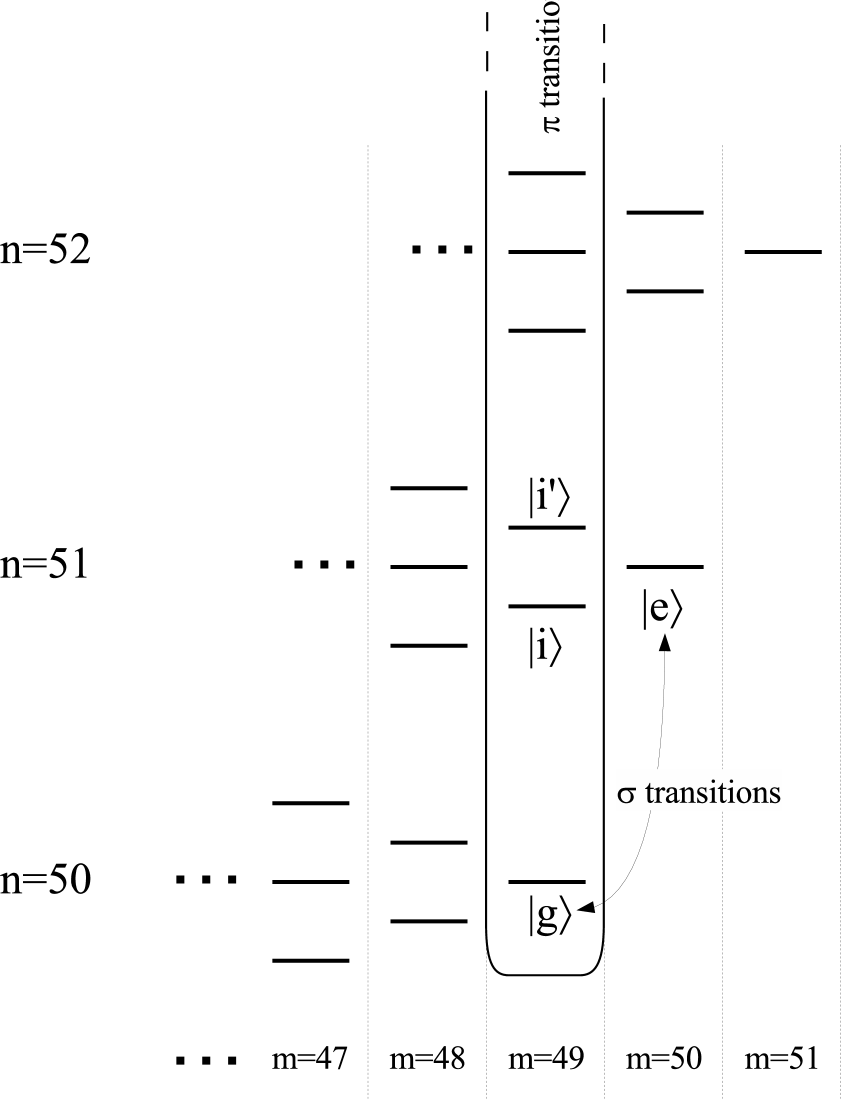
Figure 1: Level spectrum in presence of an electric field for the multiplicities $n=50,51$ and $52$. Only the levels with the largest angular momentum are presented ($m\geq n-3$). A $\pi$-polarized microwave field will couple levels of equal $m$, for example those of $m=49$ separated from the others by a box in this figure. A $\sigma$-polarized microwave field will, in contrast, couple levels of $m$ differing by $\pm 1$, for example levels $|g\rangle$ and $|e\rangle$.

Fig. 1 presents the energy levels in the presence of an electric field for the principal quantum numbers $n$ relevant to our discussion. It is important to note that circular states, having no permanent mean electric dipole, experience no linear Stark effect ($\mathcal{E}^{(1)}=0$). They are, however, much more highly polarizable than ground state atoms and have an accordingly large quadratic Stark effect [$\mathcal{E}_{i}\approx\alpha_{i}E^{2}$ for $i=(g,e)$, where $\alpha_{i}$ is half the polarizability]. Its value, $\alpha_{g}=-203,2$ Hz/(V/m)² for $n=50$ and $\alpha_{e}=-228,7$ Hz/(V/m)² for $n=51$, is 9 orders of magnitude larger than that of the ground state of Hydrogen. Nonetheless, circular states are high-field seekers and cannot therefore be trapped by any configuration of d.c. electric fields, a maximum of the electric field modulus in vacuum being forbidden by Maxwell’s equations.

2.2 Trapping

A similar situation is encountered in the case of charged particles, such as ions. In that particular example, Maxwell’s equations prevent us from obtaining an extremum of the electric potential in a region devoid of charge. It is nevertheless possible to trap ions if one uses a.c. electric potentials, as in the case of Paul traps PAULNOBEL_80 . Building on these ideas it has been shown by Peik TR_PEIK99 that polarizable atoms can be trapped if one combines a relatively strong, d.c. and homogeneous electric field $\vec{E}_{1}=E_{1}\vec{u}_{z}$ (where $\vec{u}_{z}$ is a unit vector along the vertical) and an inhomogeneous a.c. field $\vec{E}_{3}(\vec{r},t)$ deriving from a time-varying hexapolar potential. As a first step we consider the case where $E_{3}\ll E_{1}$. The field is therefore almost homogeneous over the trapping region and small departures from $\vec{E}_{1}$ are responsible for the confinement. Let $V_{1}(\vec{r})$ and $V_{3}(\vec{r},t)$ be the potentials associated to $\vec{E}_{1}$ and $\vec{E}_{3}(\vec{r},t)$ respectively. One can write these potentials in the form:

$$V_{1}(x,y,z) = \frac{U_{1}z}{z_{0}},$$ (5)

$$V_{3}(x,y,z,t) = \frac{U_{3}(t)}{2z_{0}^{3}}(2z^{3}-3zx^{2}-3zy^{2}),$$ (6)

where the $U_{i}$ are quantities homogeneous to electric potentials and $z_{0}$ is a length of the order of the electrode size. If one considers a circular Rydberg atom following adiabatically the electric field variations, its potential energy in the quadratic Stark approximation is given by:

$$\mathcal{E} = \alpha|\vec{E}_{1}+\vec{E}_{3}|^{2}$$ (7)

$$= \alpha(E_{1}^{2}+2\vec{E}_{1}\cdot\vec{E}_{3}+E_{3}^{2}).$$

Assuming $E_{3}\ll E_{1}$ and neglecting the constant terms in the potential energy we arrive at:

$$\mathcal{E} \simeq 2\alpha E_{1}\vec{E}_{3}\cdot\vec{u}_{z}$$ (8)

$$\simeq 2\alpha\frac{U_{1}}{z_{0}}\frac{\partial V_{3}(x,y,z,t)}{\partial z}$$

$$\simeq \alpha\frac{3U_{1}U_{3}(t)}{z_{0}^{4}}(2z^{2}-x^{2}-y^{2}).$$

We see that we now have an expression for the potential energy quadratic in $x$, $y$ and $z$, as in conventional ion traps. It is important to note that if we have trapping along directions $x$ and $y$ (i.e. $U_{1}U_{3}(t)>0\mbox{ for }\alpha<0$) then we necessarily have antitrapping along direction $z$, and vice versa. Moreover, if $U_{3}$ varies sinusoidally [i.e. $U_{3}(t)=U_{30}\cos(\omega t)$] then the equation of motion along $Ox$ can be written:

$$m_{Rb}\frac{d^{2}x}{dt^{2}}-\frac{6\alpha U_{1}U_{30}}{z_{0}^{4}}\cos(\omega t)x=0.$$ (9)

Equation 9 can be transformed into the well known Mathieu form:

$$\frac{d^{2}x}{d\tau^{2}}-2q_{x}\cos(2\tau)x=0,$$ (10)

where $\tau=\omega t/2$ et $q_{x}=12\alpha U_{1}U_{30}/m_{Rb}\omega^{2}z_{0}^{4}$.

The equation of motion is of the same form along the other directions with $q_{y}=q_{x}$ and $q_{z}=-2q_{x}$. There exists a stable solution, confined in space, if $|q_{i}|\leq 0.907,\ i=x,y,z$.

In order to compensate the force of gravity, taken to be along $-z$, it is also possible to add to $V_{1}$ and $V_{3}$ a d.c. quadrupolar potential $V_{2}(\vec{r})=U_{2}(x^{2}+y^{2}-2z^{2})/z_{0}^{2}$. If $U_{2}\ll U_{1}$, the same analysis as before, considering only the terms in $U_{1}$ and $U_{2}$, leads to:

$$\mathcal{E} \simeq 2\alpha\frac{U_{1}}{z_{0}}\frac{\partial V_{2}(x,y,z)}{\partial z}$$ (11)

$$\simeq -4\alpha\frac{U_{1}U_{2}}{z_{0}^{3}}z,$$

compensating gravity if $U_{2}=mgz_{0}^{3}/4\alpha U_{1}$.

2.3 Proposed geometries, calculation of potentials and fields

It is of course possible to design a geometry of electrodes which perfectly maps the desired hexapolar geometry [see Fig. 2 (a)]. It requires two rings and two end caps. However, being closed in all three dimensions, such a geometry is hardly compatible with efficient atom loading, nor with the idea of building all the trapping components on a microfabricated structure. We propose instead a design (trap A) based on two chips facing each other [see Fig. 2 (b)]. Each chip could be made by standard lithographic methods and consists of two electrodes: a disk, playing the role of end cap, surrounded by a plane. The diameter of the disks is 1 mm and the outer electrodes would extend to $y=\pm 1\mbox{~{}cm}$ and even further in $x$, the electrodes forming part of a long waveguide (see Sec. 5.2). To ease the numerical calculation of the potentials we cut the electrodes off at $\rho=\sqrt{x^{2}+y^{2}}=2\mbox{~{}mm}$ and confirmed afterwards that this had a negligible effect upon the potential within the trapping region.

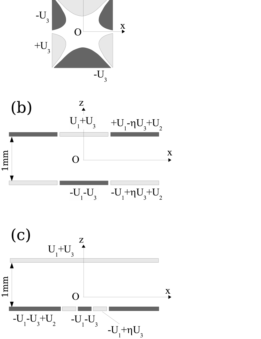
Figure 2: For all figures there is a cylindrical symmetry around $Oz$ and the electrodes are shaded according to the phase of the oscillating potential $U_{3}$. (a) Electrode geometry creating an exact hexapolar potential. (b) Section of trap A in a vertical $xOz$ plane, with applied potentials. The diameter of the inner electrode is 1 mm. The plate spacing, 1 mm, is appropriate for spontaneous emission inhibition. The analogy with the geometry of (a) is conspicuous. (c) Geometry of trap B. The lower plane is not drawn to scale, the inner disk electrode having a diameter of 100 $\mu$m and the ring around it being of width 100 $\mu$m. The plate spacing remains 1 mm.

The voltage applied to each electrode is the sum of 3 terms:

• A static voltage $\pm U_{1}$ creating a homogeneous field $\vec{E}_{1}$ along $Oz$, as in a plane capacitor.

• A static voltage $U_{2}$ on the outer ring of both chips creating a potential with a large quadrupolar component of the same form as $V_{2}(\vec{r})$. This component, in conjunction with $\vec{E}_{1}$ as seen above, will create a force on the atom compensating gravity.

• A time-varying voltage $U_{3}(t)$ creating a potential with a large hexapolar component of the same form as $V_{3}(\vec{r},t)$. This component, in conjunction with $\vec{E}_{1}$ as seen above, allows for trapping.

It is, however, important to note that the electric potential associated to $U_{2}$ (resp. $U_{3}$) is clearly not an ideal quadrupole (resp. hexapole). The resulting electric fields are therefore more complicated. As an illustration, if the factor $\eta$ of Fig. 2 (b) is set equal to 1, $U_{3}$ will create a non-zero electric field along $Oz$ at the centre of the trap $O$. This will create a time-varying electric field, and therefore atomic energy, at trap centre, resulting in heating. A correct choice of $\eta$ allows us to better approximate a perfectly hexapolar potential, and cancel this electric field.

More specifically, our final goal is to be able to calculate the electric field at any position inside the trap and at any time. Moreover, it is important to assess edge effects as well as the effects of the finite gap between the electrodes. We have therefore opted for a numerical approach. We numerically calculate the potential inside the trap on a grid of points using the software SIMION SIMION . In order to limit numerical errors in the calculation of the gradient we then make a fit of the potential on the basis of the first seven spherical harmonics $Y_{l}^{m}(\theta,\phi)$, centred on $O$. Due to the cylindrical symmetry around $Oz$ only the $m=0$ terms are present. Thanks to the linearity of Maxwell’s equations one can add separately the contribution of each voltage $U_{k}\ (k=1,2,3)$ and we therefore have, neglecting the physically unimportant constant term:

$$V_{\mbox{\tiny{Fit}}}(r,\theta,\phi,t)=\sum_{l=1}^{7}\sum_{k=1}^{3}v_{kl}U_{k}(t)\left(\frac{r}{z_{0}}\right)^{l}Y_{l}^{0}(\theta),$$ (12)

where $z_{0}$ is an arbitrary length, chosen to be characteristic of the trap geometry, and set equal to 1 mm for trap A. The parameters $v_{kl}$ only depend on the geometry of the electrodes and are determined from our fit on the numerically calculated grid. Due to symmetries one can set $v_{1l}=0$ for $l\geq 2$, $v_{2l}=0$ for $l$ odd and $v_{3l}=0$ for $l$ even. The results of the fits are presented in Table 1. The relative difference between the results of SIMION and the fit is smaller than 1% within a radius of 400 $\mu$m from $O$.

$k\backslash l$	1	2	3	4	5	6	7
$1$	4.09	0	0	0	0	0	0
$2$	0	-3.12	0	-0.63	0	3.73	0
$3\ (\eta=1)$	2.60	0	5.48	0	-3.66	0	-5.75
$3\ (\eta=4.49)$	0	0	15.04	0	-10.05	0	-15.76

Table 1: Results of the fit of the potential coefficients $v_{kl}$ for trap A ($z_{0}=1\mbox{~{}mm}$). The first two lines give values for the fit of applied voltages $U_{1}$ and $U_{2}$ respectively, the third line for applied voltage $U_{3}$ with $\eta=1$. It is possible to cancel the electric field created by $U_{3}$ at the centre of the trap by setting $\eta=4.49$ (fourth line)

We have also designed another trap geometry (trap B) which achieves tighter confinement and smaller atom-electrode distances [see Fig. 2(c)]. Such a setup is necessary for atom-surface interaction studies. Trap B is derived from trap A by bringing the ring of the top plane of Fig. 2(b) down onto the lower plane. The electrode size is reduced by a factor of 10 (and $z_{0}$ accordingly reduced to $100~{}\mu$m) while the distance between the two planes remains unchanged at 1 mm. Numerical calculations with SIMION show that there exists a saddle point for the electric field modulus at a point $O$, 120 $\mu$m above the lower plane surface. It is possible to apply the same numerical treatment to this trap as before and fit the electric potential around $O$ (here however we have fewer symmetries and can consequently set fewer of the $v_{kl}$ equal to zero). This procedure produces a fit correct to 0.1% within a radius of 50 $\mu$m of $O$. The results are shown in Table 2.

tabularc—ccccccc $k\backslash l$ 1 2 3 4 5 6 7
$1$ 0.409 0 0 0 0 0 0
$2$ 0.457 -0.220 0.037 0.010 -0.010 0.001 2$\times$10^-6
$3\ (\eta=1)$ -0.369 0.002 0.250 -0.241 0.155 -0.075 -0.027
$3\ (\eta=0.05)$ 0 0.001 0.131 -0.127 0.082 -0.039 -0.014

Table 2: Results of the fit of the potential coefficients $v_{kl}$ for trap B ($z_{0}=100~{}\mu\mbox{m}$). The different lines have the same meaning as in Table 1.

2.4 Simulation of trajectories

The evolution of the atom in the time-varying electric field being adiabatic (see Sec. 2.1) we can simply write $\mathcal{E}(t)=\mathcal{E}[E(t)]$. From $V_{\mbox{\tiny{Fit}}}$, it is easy to derive a formula for the electric field modulus $E$, and therefore for the potential energy of a trapped atom. It is then simple to derive an expression for the force on the atom along each direction.

In the case of trap A, due to its symmetries, the potential energy considered as a power series in $|\vec{r}|$ has a small number of terms that dominate. The first non-trivial term is a quadrupolar term, exactly equivalent to (8):

$$\mathcal{E}^{\mbox{\tiny{Quad}}}=\alpha~{}\frac{3\sqrt{21}}{4\pi}\frac{U_{1}U_{3}(t)v_{11}v_{22}}{z_{0}^{4}}~{}(2z^{2}-x^{2}-y^{2}).\\$$ (13)

If, once again, we have $U_{3}(t)=U_{30}\cos(\omega t)$ then for each direction the associated Mathieu equation will have a characteristic parameter $q_{i}\ (i=x,y,z)$ equal to:

$$q_{x}=q_{y} = \alpha\frac{3\sqrt{21}}{\pi}\frac{U_{1}U_{30}v_{11}v_{33}}{m_{Rb}\omega^{2}z_{0}^{4}},$$ (14)

$$q_{z} = -2q_{x}.$$ (15)

The second non-trivial term is a term linear in $z$, exactly equivalent to (11):

$$\mathcal{E}^{\mbox{\tiny{Lin}}}=\alpha~{}\frac{\sqrt{15}}{\pi}\frac{U_{1}U_{2}v_{11}v_{22}}{z_{0}^{3}}~{}z,$$ (16)

allowing us to calculate the value of $U_{2}$ necessary to compensate gravity.

The use of only these first two terms fits the exact potential energy to better than 1% within 100 $\mu$m of $O$ and allows one to find solutions for the trajectories via analysis of the Mathieu equation. This treatment, however, does not suffice for trap B due to its non-zero values of $v_{21}$ and $v_{32}$. Therefore, to treat trap B, and to achieve a more precise calculation of the trajectories, we retain a full numerical approach:

• Each trajectory is computed, using an adaptive Runge-Kutta algorithm.

• The total time over which we calculate the trajectories ranges from a few ms to several seconds according to the application.

• A trajectory is considered trapped if the atom remains within the sphere of validity of the numerical fit of the potential (radius of 400 $\mu$m for trap A, 50 $\mu$m for trap B). 99% of untrapped atoms leave this zone within 0.55 s.

• We use initial conditions for the velocity and position of the trapped atom coherent with excitation from a trapped cloud of Rubidium atoms (trapping frequency 1 kHz along each direction) at thermal equilibrium (temperature $T_{0}=300$ nK) and with the loading mechanism that we consider in Sec. 3.2. These correspond to Gaussian distributions of widths 5.35 mm/s and 0.27 $\mu$m for the velocity and position respectively. To the initial velocity is added the single recoil velocity $v_{r}=6$ mm/s along the direction $Oy$ that would be received on efficient adiabatic excitation to the Rydberg state. This temperature and trap frequency correspond to an atomic cloud close to condensation, or already condensed (average phonon number $n_{ph}\approx 6$). The initial conditions that we have taken remain valid however, as long as the number of atoms in the trap is low enough for mean field interactions between ground-state atoms to be neglected.

• For each trajectory we record periodically the atomic position and velocity, as well as the value of the electric field modulus and its direction.

In all cases we check in the shallow electrodynamic trap that the trajectory extension, of a much greater size than the initial, tightly confined ground-state cloud, is also much larger that the typical de Broglie wavelength of the atom (of the order of 0.50 $\mu$m). This justifies a classical calculation of the motion.

2.5 Trap performance

We have studied the trapping characteristics for a wide range of parameters, especially the voltage $U_{1}$ which controls the mean electric field experienced by the atoms, the voltage $U_{30}$ and the frequency $\omega$ of the a.c. field, the last two together controlling the confinement. For all of these parameters we find qualitatively the results predicted by the Mathieu equation. Bound trajectories are found to be composed of two motions: a fast micromotion, of frequency $\omega$ and of relatively small amplitude, and a slower macromotion of larger amplitude and of frequency $\omega_{x}=\omega_{y}\approx\omega_{z}/2$, an order of magnitude slower than $\omega$ (see Fig. 3). In the case of non-bound trajectories, the amplitude of the macromotion usually increases slowly until the atom is finally expelled from the region in which $V_{\mbox{\tiny{Fit}}}$ is valid.

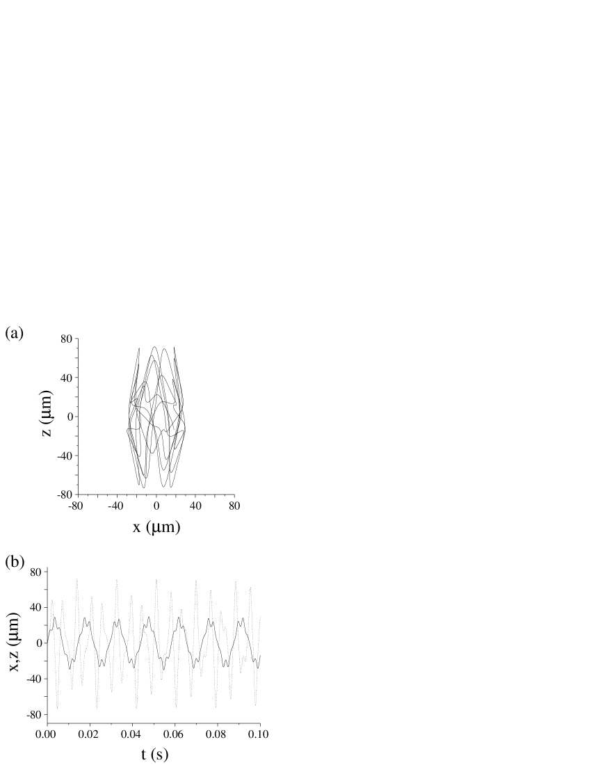
Figure 3: (a) A typical trajectory of an atom in trap A, shown in the $x0z$ plane. The atom is initially at the origin of the trap and has a velocity (12,0,12) mm/s. (b) $x$ (solid line) and $z$ (dotted line) coordinates for the same trajectory as a function of time.

The trapping efficiency as a function of the frequency $\omega$ is obtained by simulating 100 trajectories and recording the fraction of them remaining trapped after 1 s. The results for trap A are shown in Fig. 4. No trapping is possible below a threshold frequency $\omega_{th}/2\pi$. This is in qualitative agreement with the prediction of the Mathieu equation stability criteria $|q_{z}|<0.907$. For the parameters of Fig. 4 this would set a threshold frequency at 395 Hz, compared to the value of $\omega_{th}/2\pi=$400 Hz found in the simulations. Just above $\omega_{th}$ the efficiency depends essentially on the initial temperature $T_{0}$ of the sample and can be very close to 100% for comparatively cold atoms. If one continues to increase $\omega$ one observes a slow decay of the efficiency. This can be easily understood as due to the increasing ‘averaging’ of the time-dependent electric field seen by the atom. The Mathieu equation predicts that the macromotion frequencies $\omega_{x}$, $\omega_{y}$ and $\omega_{z}$ decrease as $1/\omega$. There will therefore rapidly come a point when $\omega$ is so much larger than $\omega_{x}$, $\omega_{y}$ and $\omega_{z}$ that the time-dependent field $\vec{E}_{3}(\vec{r},t)$ averages completely and the atom, seeing a homogeneous field, is no longer trapped.

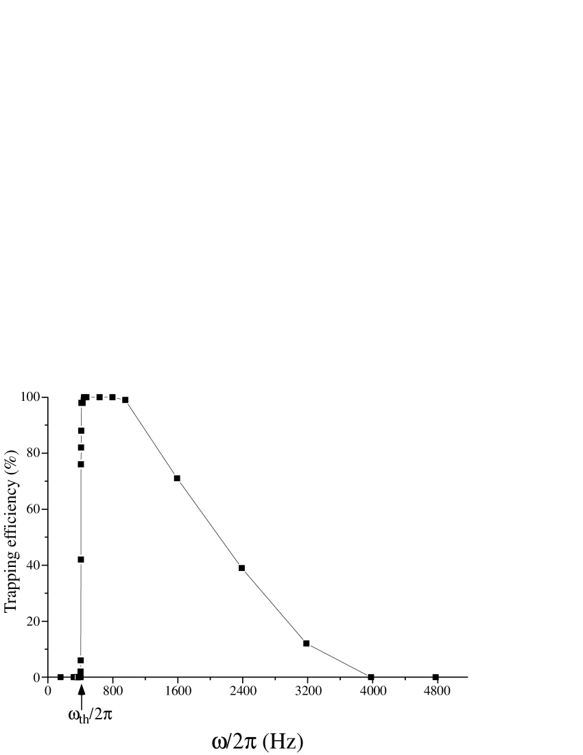
Figure 4: Trapping efficiency (trap A) as a function of frequency $\omega$. $U_{1}=$0.2 V, $U_{2}=-3$ mV, $U_{30}=$0.056 V, $T_{0}$=1 $\mu$K.

In the following, $\omega$ will be chosen slightly above $\omega_{th}$ where the trapping efficiency is largest. Although this does not correspond to a situation where a clear cut separation of the micro- and macromotions exists, we can still distinguish between the two. We present in Table 3 the frequencies of the macromotion $\omega_{\rho}=\omega_{x}=\omega_{y}$ and $\omega_{z}$ for different geometries and sets of voltages. In order to estimate the depth of each trap we calculate the trapping efficiency for different initial temperatures. We define $T_{d}$ as the temperature above which more than 50% of the atoms are lost after 1 s. For trap B, two values of $U_{1}$ are shown (0.2 and 1.5 V), corresponding to two different bias electric field amplitudes. Comparison of the results clearly show that the smaller the trap and the larger the bias field the tighter the confinement. Trap depth can reach as high as the mK with motion frequencies in the kHz range. However, most of the following simulations have been performed with a small voltage $U_{1}$, necessary for studies of coherent superpositions of $|g\rangle$ and $|e\rangle$, as we shall see in Sec. 5. Even in these unfavourable conditions for trapping, the depths attained are compatible with typical cold-atom temperatures and oscillation frequencies remain reasonable, around 100 Hz.

Small departures of the electric field direction from $\vec{u}_{z}$ in the trapping region, due to transverse components of $\vec{E}_{2}$ and $\vec{E}_{3}$, will later prove critical in calculating the efficiency of the spontaneous emission inhibition (Sec. 4) and the rate of dephasing between $|g\rangle$ and $|e\rangle$ (Sec. 5). We therefore note in Table 3 the mean angle $\langle\theta\rangle$ between the local electric field and $\vec{u}_{z}$ experienced by an atom over the course of its trajectory.

Type	$\eta$	$U_{1}$ (V)	$U_{30}$ (V)	$U_{2}$ (mV)	$\omega/2\pi$ (Hz)	$\omega_{\rho}/2\pi$ (Hz)	$\omega_{z}/2\pi$ (Hz)	$T_{d}$ ($\mu$K)	$\langle\theta\rangle$ (mRad)
Trap $A$	4.49	0.2	0.056	-3	430	64	175	180	9.38
Trap $B$-$\alpha$	0.05	1.5	0.5	0	20700	1460	2910	1000	4.22
Trap $B$-$\beta$	0.05	0.2	0.14	-0.45	2860	207	414	35	3.57

Table 3: Trap $A$ and trap $B$ correspond to the geometries of Fig. 2(b) and (c) respectively. Labels $\alpha$ and $\beta$ for Trap $B$ correspond to different voltage settings. For each trap, we give the values for $U_{1}$, $U_{2}$, $U_{30}$ and the frequency $\omega/2\pi$. The frequencies $\omega_{z}/2\pi$ and $\omega_{\rho}/2\pi$ are the typical longitudinal (along $Oz$) and transverse oscillation frequencies in the trap. The trap depth $T_{d}$ is defined as the temperature for which half of the atoms remain trapped. $\langle\theta\rangle$ is the mean angle between the local electric field $\vec{E}$ and $\vec{u}_{z}$, averaged over 100 trajectories at temperature $T_{d}/2$.

3 Loading of the trap, preparation of a subpoissonian sample of Rydberg atoms

3.1 The dipole-blockade effect

For many quantum information processing experiments, the deterministic preparation and storage of an individual qubit is a critical requirement. This has already been achieved, for example, with trapped ions. In previous experiments with circular Rydberg atoms ENS_RMP , we expressly set the rate of excitation extremely low in order to be able to neglect two-atom events. This is, of course, at the expense of very long data acquisition times. We propose here to deterministically load the trap with a single Rydberg atom by using the dipole-blockade effect. This phenomenon has been proposed as an efficient way to perform quantum gates between two Rydberg atoms QI_LUKINDIPOLEBLOCKADE01 but can also ensure the preparation of one and only one low angular momentum Rydberg state by laser excitation of a dense micron-sized cloud of ground-state atoms TR_SAFFMANN02 . The essential idea behind this phenomenon is that level shifts due to the dipole-dipole interaction make the laser nonresonant for the excitation of more than one Rydberg atom.

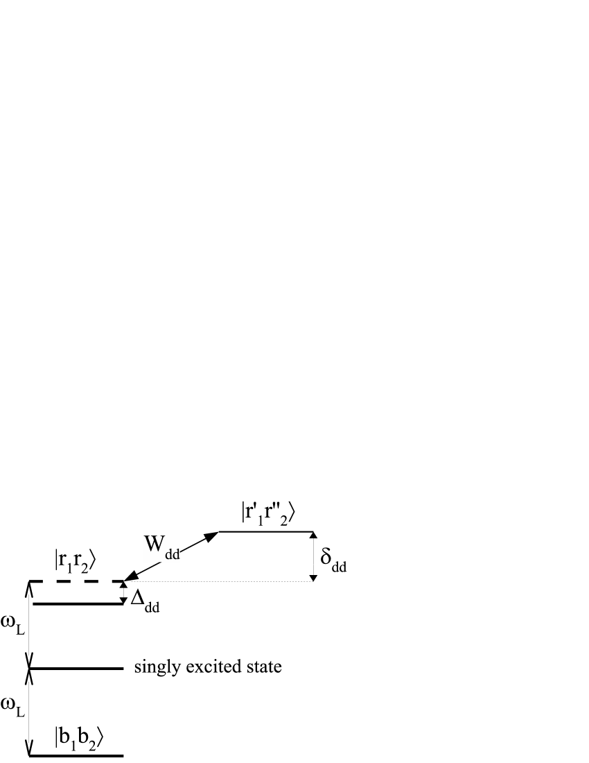
Figure 5: Level diagram demonstrating the dipole-blockade effect.

In order to assess the effect of atom-atom interactions we consider an ensemble of $N$ cold ground-state atoms (temperature in the $\mu$K range) in the presence of a laser resonant with the transition between a low-lying state $|b\rangle$ and a given Rydberg state $|r\rangle$. Atomic motion can be neglected during the laser excitation and hence each atom position $\vec{R}_{i}$ is treated as fixed. Let us assume that the initial trap confines the atoms in a micron-sized region such that $|\vec{R}_{ij}|=|\vec{R}_{i}-\vec{R}_{j}|<1\ \mu$m for any couple $(i,j)$ of atoms. We then switch on the laser light, of frequency $\omega_{L}$.

Let us consider for a moment only atoms 1 and 2. Fig. 5 shows the relevant levels for this simplified situation. We tune the laser frequency to be resonant on the transition from the lower state $|b_{1}b_{2}\rangle$ to the singly excited state, where one of the atoms has been excited to the Rydberg state $|r\rangle$. In the absence of interactions, this laser would also be resonant with the transition towards the state $|r_{1}r_{2}\rangle$ where both atoms 1 and 2 are excited into the state $|r\rangle$. We must, however, take into account the coupling of this level $|r_{1}r_{2}\rangle$ with other doubly excited states of different Rydberg levels, for example $|r_{1}^{\prime}r_{2}^{\prime\prime}\rangle$, shifted in energy from $|r_{1}r_{2}\rangle$ by $\delta_{dd}$ (see Fig. 5). This coupling, of magnitude $W_{dd}$, will cause a shift $\Delta_{dd}$ of the level $|r_{1}r_{2}\rangle$ which, if large enough, will make the excitation of the doubly excited level nonresonant and therefore strongly suppressed. We must therefore calculate $\Delta_{dd}$. First order perturbation theory gives us:

$$\Delta_{dd}=\frac{W_{dd}^{2}}{\delta_{dd}}.$$ (17)

$\delta_{dd}$ will be of the order of the separation of Rydberg levels, a few GHz for $n\sim 50$. A classical order of magnitude for $W_{dd}$ is given by:

$$hW_{\mbox{\tiny{dd}}}=\frac{n^{4}e^{2}a_{0}^{2}}{8\pi\epsilon_{0}|\vec{R}_{12}|^{3}},$$ (18)

where $a_{0}$ is the Bohr radius. For a distance $|\vec{R}_{12}|=1\ \mu$m and $n=50$ one calculates $W_{\mbox{\tiny{dd}}}=3$ GHz. We therefore calculate a shift of the doubly excited level $\Delta_{dd}\sim$ 1 GHz. This order of magnitude calculation is in agreement with the result $\Delta_{dd}=100$ MHz found by Saffmann and Walker TR_SAFFMANN02 . This shift is easily resolved using modern lasers and hence excitation of multiple Rydberg atoms will be out of resonance with the excitation laser. It is shown in TR_SAFFMANN02 that for the resonant excitation of the transition $|b\rangle\longrightarrow|r\rangle$ in a cloud of ground state atoms of diametre 5 $\mu$m using a laser of Rabi frequency 1 MHz one obtains multiple- or non-excitation of $|r\rangle$ for less than 1 event in $10^{4}$ (for a number of ground-state atoms of the order of a few hundred, compatible with the assumption that we can neglect interactions in the calculation of the initial conditions).

3.2 Loading from a magnetic atom-chip trap

Atom-chip traps MX_HANSCHCHIP99 can fulfill all the conditions required by our proposal. They allow for very high densities of ground-state atoms in trap volumes as small as a few $\mu$m³ FOLMANCHIPREV_02 . They can, by construction, store atoms close to surfaces and the operation of a conveyor belt, ideal for bringing atoms from a capture region into the Rydberg trap, has been proven TR_CONVEYOR_REICHEL01 . Finally, evaporative cooling in such traps allows one to attain temperatures as low as a few hundred nK MX_HANSCHBECCHIP01 . The need for operation at cryogenic temperatures, in order to get rid of blackbody radiation which would rapidly destabilize the Rydberg states (see Sec. 4), makes it impossible however to use standard atom-chip designs with normal conductors. We plan to use instead superconductors to create the magnetic fields. This would allow us to pass current without Joule heating as long as one remains below the critical current. In standard atom-chip experiments at room temperature the current densities are typically of the order of $5\times 10^{6}$ Acm^-2 SCHMIEDMAYERCHIPFAB_04 . We have checked that it is possible to reach similar current densities with our superconducting wires. In the case of a superconducting Niobium wire of thickness 1 $\mu$m and width 10 $\mu$m, sputtered on a Silicon Oxide substrate, we find $I_{c}=0.5$ A, corresponding to a current density of $5\times 10^{6}$ Acm^-2.

Thanks to our microfabricated design, it is simple to integrate our Rydberg trap with the magnetic atom-chip trap and also the electrodes necessary for the transfer of the atom from a low angular momentum Rydberg state to a circular state ENS_CIRCRB . We have designed a multi-layer configuration with the electrodes necessary for the Rydberg trap placed on top of the wires of the magnetic atom chip. The circularization is achieved using wires on the magnetic atom-chip layer to create the necessary magnetic field along with the application of a r.f. voltage to electrodes on the Rydberg trap layer. The Rydberg trap electrodes will not significantly affect the magnetic field created by the wires of the lower layer as long as a normal conductor such as Gold is used. Evaporative cooling in the magnetic atom-chip trap can provide a few hundred atoms in a micron-sized cloud at temperatures as low as a few hundred nK MX_HANSCHBECCHIP01 , conditions ideal for the operation of the dipole-blockade effect. The magnetic trap is then suddenly switched off and the excitation towards a low angular momentum Rydberg state performed immediately. Carefully designed laser excitation schemes result in the atom receiving only one optical photon recoil, just before the circularization process, itself lasting about 20 $\mu$s ENS_CIRCRB ; ENS_RMP . The flexibility of magnetic atom chips will allow us to superimpose the centre of the magnetic trap with that of the Rydberg trap.

4 Making the atom long-lived by spontaneous emission inhibition

4.1 Principles

The basic idea behind the inhibition of spontaneous emission is to place the atom inside a cavity containing no mode into which the atom can emit its photon upon decay ENS_HOUCHES90 . For the sake of simplicity we first of all consider the geometry of Fig. 6 where a circular Rydberg atom is placed between two infinite, perfectly conducting planes separated by a distance $L$. This situation is relatively close to that of Fig. 2 (b). We now assume that there exists between the two planes a d.c. electric field $\vec{E}_{\mbox{\tiny{dir}}}$ orthogonal to the planes (and hence parallel to their normal $\vec{u}_{z}$). Obeying the standard selection rules, a circular Rydberg state of principal quantum number $n$ possesses only a single possible decay channel, this being towards the lower circular state $n-1$ (for example $|e\rangle\rightarrow|g\rangle$). In the process it emits a photon of polarization $\sigma^{+}$ with respect to $\vec{u}_{z}$, of wavelength $\lambda_{sp}$ ($\lambda_{sp}\simeq 6$ mm for the decay of $|g\rangle$ and $|e\rangle$). Due to its polarization, the electric field associated with this photon is perpendicular to $\vec{u}_{z}$ and hence parallel to the planes. The maximum wavelength of any such mode inside this cavity is $2L$ as the electric field must cancel at the surface of each plane. Therefore, if $\lambda_{sp}>2L$, there exists no cavity mode at resonance with the spontaneous emission transition and the atom cannot decay, remaining in the circular state for an infinitely long time.

Figure 6: Ideal geometry for spontaneous emission inhibition.

We now detail a more rigorous, semi-classical approach to this phenomenon, as found in Ref. ENS_HOUCHES90 . We calculate the effect of the field radiated by the dipole upon itself, and hence the consequent energy shifts and lifetimes. The electric field radiated by a dipole $\vec{D}=D\exp(-i\omega t)\vec{u}_{d}$ at position $\vec{r}_{d}$ oscillating at frequency $\omega$ along unit vector $\vec{u}_{d}$ is given by:

$$\vec{E}_{dip}(\vec{r},t)=\frac{D\omega^{3}}{4\pi\epsilon_{0}c^{3}}\bm{\mathcal{F}}^{(cav)}(\vec{r},\vec{r}_{d},\omega)e^{-i\omega t},$$ (19)

where $\bm{\mathcal{F}}^{(cav)}(\vec{r},\vec{r}_{d},\omega)$ is the susceptibility of the field inside the cavity, characterizing the linear response of the system to the dipole movement. This susceptibility can be written in the form:

$$\bm{\mathcal{F}}^{(cav)}(\vec{r},\vec{r}_{d},\omega)=\bm{\mathcal{F}}^{(0)}(\vec{r},\vec{r}_{d},\omega)+\bm{\mathcal{F}}^{(r)}(\vec{r},\vec{r}_{d},\omega).$$ (20)

The field corresponding to $\bm{\mathcal{F}}^{(0)}(\vec{r},\vec{r}_{d},\omega)$ is the field radiated by the dipole in free space and that corresponding to $\bm{\mathcal{F}}^{(r)}(\vec{r},\vec{r}_{d},\omega)$ reflects the modification introduced by the presence of the cavity and is easily understood as being the field radiated by the images of the dipole in the surfaces of the cavity. When we calculate the interaction of the dipole with the total field we will therefore have two terms:

• A first representing the interaction of the dipole with its own free space field. This term leads us to the calculation of the natural lifetime of the dipole and the Lamb shift of its frequency. This calculation however is plagued by divergences. Their values must be derived by a fully quantum treatment, and we simply insert these results into our calculation.

• A second corresponding to the interaction of the dipole with the field of its images. This leads to the modification of the natural lifetime (that we search to calculate) along with the accompanying frequency shift. Its calculation, in contrast to the first, poses no problem.

This approach gives the following expression for the rate of decay of the dipole (atom) inside the cavity ENS_HOUCHES90 :

$$\Gamma=\Gamma_{0}\left(1+\frac{3}{2}\mbox{Im}\left[\vec{u}_{d}.\bm{\mathcal{F}}^{(r)}(\vec{r}_{d},\vec{r}_{d},\omega)\right]\right),$$ (21)

the imaginary part of the susceptibility corresponding to the component of the image field in quadrature with the dipole oscillation and hence responsible for dissipation. We present in Fig. 7 the evolution of the ratio $\Gamma/\Gamma_{0}$ as a function of the distance $L$ in two specific situations: $\vec{D}$ parallel to $\vec{u}_{z}$; $\vec{D}$ perpendicular to $\vec{u}_{z}$. In the latter, the case of $\sigma$ emission in the presence of a quantization axis along $\vec{u}_{z}$, one observes a complete inhibition for $L<\lambda/2$. In the former, the case of $\pi$ emission in the presence of the same quantization axis along $\vec{u}_{z}$, the dipole couples to modes obeying different boundary conditions and its emission is exalted for small $L$ values. In the case of a $\sigma$ transition in the presence of a quantization axis slightly tilted with respect to $\vec{u}_{z}$ we have components of $\vec{D}$ both parallel and perpendicular to $\vec{u}_{z}$ and consequently the possibility of decay via both inhibited and exalted channels.

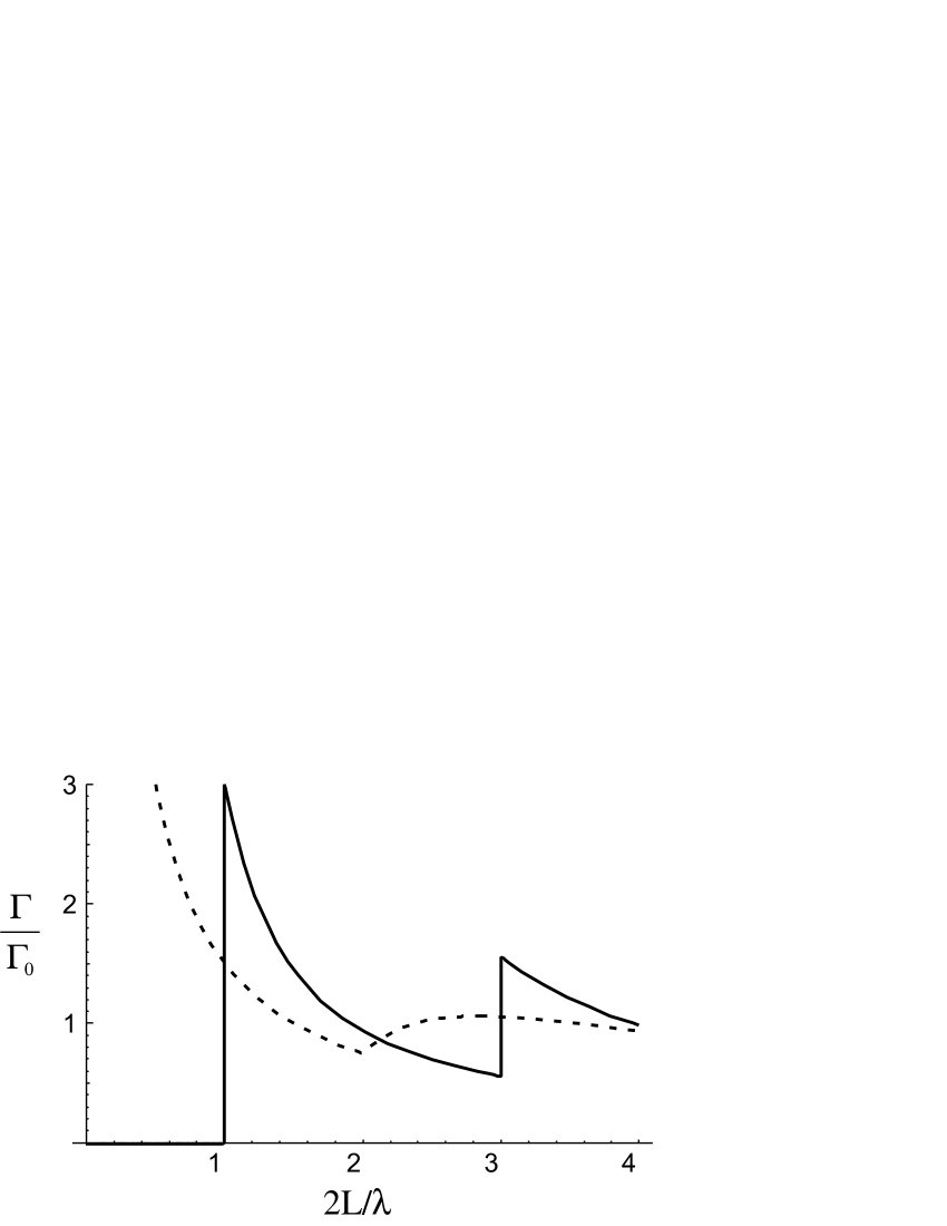
Figure 7: Spontaneous emission rate $\Gamma$, in units of $\Gamma_{0}$, as a function of the cavity plane separation $L$. The dipole is either parallel to the mirrors ($\Gamma_{\parallel}$, continuous line) or perpendicular to them ($\Gamma_{\perp}$, dashed line). Both are calculated for the case of perfectly conducting mirrors.

Inhibition has already been observed in the microwave domain QC_KLEPPNERINHIBITION85 as well as for optical transitions QC_YALEOPTICALINHIB87 . A value of less than 0.1 for $\Gamma/\Gamma_{0}$ has been reported in the case of Rydberg atoms. This would already increase the radiative lifetime of circular states to a significant fraction of a second.

4.2 Limitations of the inhibition

The ideal case presented in Sec. 4.1 is, however, far from the realistic geometries of Fig. 2(b) and (c), the imperfections of which we must now evaluate. As a first example, the electrodes do not form perfect infinite mirrors. It is possible to neglect the effect of their finite size if, as will be the case, the transverse dimensions of the trap are much larger than $\lambda_{sp}$. A more critical effect comes from the residual absorption by the imperfect mirrors, dissipating the energy radiated by the atom and limiting its lifetime. This effect must therefore be included in the calculation of the susceptibility $\bm{\mathcal{F}}^{(r)}(\vec{r},\vec{r}_{d},\omega)$. The dipole of an image produced by a number of reflections in the mirrors $N_{R}$ is therefore multiplied by a factor:

$$(\rho e^{i\chi})^{N_{R}},$$ (22)

where $|\rho|^{2}$ is the reflection coefficient of the mirror and $\chi$ accounts for the phase shift at each reflection. For trapping electrodes made of ordinary conductors (such as Gold) $\rho$ and $\chi$ are related to the skin depth $\delta$ by the following expressions:

$$\rho \simeq \exp(-\frac{2\pi\delta}{\lambda}),$$ (23)

$$\chi \simeq \frac{2\pi\delta}{\lambda},$$ (24)

provided that, as is the case here, $\delta\ll\lambda$ TXT_JACKSON . Figure 8(a) presents the inhibition factor $\Gamma_{\parallel}/\Gamma_{0}$ as a function of the skin depth $\delta$ in the case of a dipole radiating at 50 GHz ($\lambda=6$ mm). The cavity spacing $L$ is 1 mm and the dipole 120 $\mu$m away from one mirror as in trap B. One can see that inhibition is still efficient (a factor of greater than 100) for skin depths of less than 100 nm. Operating, as we must, under cryogenic conditions, we can therefore use Gold, for which $\delta=30$ nm at 1 K. For imperfect mirrors there is another effect that must be considered. The inhibition factor now depends upon the position of the atom between the two planes. Figure 8(b) shows this effect. The closer to the surfaces, the worse the inhibition. One might fear that this would pose problems in trap B. However, even in the case of a circular Rydberg atom in trap B, 120 $\mu$m away from Gold trapping electrodes at 1K, the inhibition factor of 340 would imply a radiative lifetime of 10 s.

Figure 8: (a) Spontaneous emission inhibition factor $\Gamma_{\parallel}/\Gamma_{0}$ as a function of the skin depth $\delta$. The conditions are the same as in Fig. 6 with $L=1$ mm, $\lambda=6$ mm and a dipole 120 $\mu$m away from one mirror. (b) $\Gamma_{\parallel}/\Gamma_{0}$ as a function of the atom-mirror separation for the same values of $L$ and $\lambda$ as (a) and with $\delta=30$ nm, corresponding to the case of Gold at 1 K

We must also consider the consequences of our quantization axis, following adiabatically the electric field $\vec{E}(\vec{r},t)$, being not always perfectly perpendicular to the plane mirrors. A non-zero angle $\theta(\vec{r},t)$ between $\vec{E}(\vec{r},t)$ and $\vec{u}_{z}$ will be responsible for a small component $D_{\perp}=D\sin\theta$ of the dipole being orthogonal to the mirrors (and for a reduced dipole $D_{\parallel}=D\cos\theta$ parallel to the mirrors). It is therefore possible for the atom to couple to modes possessing exalted decay. Taking into account only this decay channel, the probability for remaining in the excited state is therefore given by:

$$P = \exp\left(-\int_{\mbox{\tiny tr.}}\Gamma_{\perp}\sin^{2}\theta\left[\vec{r}(t),t\right]dt\right)$$ (25)

$$= \exp\left(-\Gamma_{0}\int_{\mbox{\tiny tr.}}\frac{\Gamma_{\perp}}{\Gamma_{0}}\sin^{2}\theta\left[\vec{r}(t),t\right]dt\right),$$

where the integral is performed along the trajectory followed by the atom.

As we have seen (Table 3), $\theta\ll 1$ for the trajectories considered and we can therefore approximate $D_{\parallel}=D$ and $\sin^{2}\theta=\theta^{2}$. From Eq. 25 one can deduce a corrected inhibition factor in $\Gamma_{\mbox{\tiny corr.}}/\Gamma_{0}$, related to the value of $\theta$ along a trajectory:

$$\frac{\Gamma_{\mbox{\tiny corr.}}}{\Gamma_{0}}=\frac{\Gamma_{\parallel}}{\Gamma_{0}}+\frac{\Gamma_{\perp}}{\Gamma_{0}}\overline{\theta^{2}},$$ (26)

where:

$$\overline{\theta^{2}}=\frac{1}{t_{tr.}}\int_{\mbox{\tiny tr.}}\theta^{2}dt,$$ (27)

is the average of the square of the angle $\theta$ over the total duration of the trajectory, $t_{tr.}$. For $L=1$ mm, $\lambda=6$ mm and $\delta=30$ nm we find an exaltation factor $\Gamma_{\perp}/\Gamma_{0}$ of 4.5, whatever the distance between the dipole and the mirrors. Under the conditions considered (Table 3), $\Gamma_{\mbox{\tiny corr.}}/\Gamma_{0}$ remains greater than 150.

The final effect that must be considered in evaluating the residual lifetime of a circular Rydberg atom in the trap is excitation by blackbody photons in the modes of the cavity. These can induce $\pi$-polarized transitions between $|g\rangle$ (resp. $|e\rangle$) and the other states of the $m=49$ (resp. $m=50$) multiplicity (for example $|g\rangle\rightarrow|i\rangle$, see Fig. 1). The rate of this process is proportional to the mean photon number $n_{t}$ at the relevant transition frequency times the relaxation rate $\Gamma_{\pi}$ for each transition, the total rate $\Gamma_{\mbox{\tiny{B.B.}}}$ being equal to the sum of all possible transitions $\Gamma_{\mbox{\tiny{B.B.}}}(k)=\sum_{k^{\prime}}n_{t}(kk^{\prime})\Gamma_{\pi}(kk^{\prime})$. We calculate $\Gamma_{\mbox{\tiny{B.B.}}}(g)=3.15~{}\mbox{s}^{-1}$ and $\Gamma_{\mbox{\tiny{B.B.}}}(e)=2.75~{}\mbox{s}^{-1}$, the effect of exaltation of $\pi$ transitions having been taken into account. If the trap is cooled down to 1 K, one has $n_{t}=0.1$ and a corresponding radiative lifetime of about 3 s, once again not a limiting factor.

5 Preserving atomic coherences over long times

To this point, we have shown that it is possible to trap a single atom in a circular Rydberg state over times in the second range. It is, however, important to see if one can manipulate and maintain its internal state with the same precision. More precisely, if we hope to use this technique in quantum information experiments or for high precision spectroscopy, it is important to verify that one can prepare an atom in a coherent superposition of states and probe its phase at a later time. In the following we will focus on the transition between the two circular states $|e\rangle$ and $|g\rangle$.

5.1 Electric shifts as the main cause of dephasing

As we saw in Sec. 2.1, the Stark polarizabilities of levels $|e\rangle$ and $|g\rangle$ are slightly different. Fig. 9 shows the energy levels as a function of the electric field amplitude. The frequency $\nu_{eg}=(\mathcal{E}_{e}-\mathcal{E}_{g})/h$ of the transition has a strong dependence on the electric field:

$$\delta\nu_{eg}=\nu_{eg}(E)-\nu_{eg}(0)=\delta\alpha_{eg}E^{2},$$ (28)

with $\delta\alpha_{eg}=-25.5\mbox{~{}Hz/(V/m)}^{2}$. If one considers the case of an atom in trap $A$ in the conditions of Table 3, prepared from a cloud at 0.3 $\mu$K, it experiences over its trajectory a mean electric field amplitude $E_{a}=400$ V/m, with an excursion of $\Delta E=\pm 1$ V/m. The corresponding frequency broadening:

$$\Delta\nu_{eg}=2\delta\alpha_{eg}E_{a}\Delta E,$$ (29)

is of the order of 20 kHz. This broadening is inhomogeneous as it is different from one trajectory to the next and could only be controlled by perfect control of the initial conditions of the atomic motion. The dephasing time associated to this motional broadening is of the order of a few tens of $\mu$s.

In addition to this dephasing, the trapping frequencies ($\omega_{\rho}$, $\omega_{z}$) for states $|e\rangle$ and $|g\rangle$ differ by about 10%. The trajectories for the two states are therefore rapidly separated (‘Stern Gerlach’ effect). Coherence would be lost when this separation exceeds the wave-packet coherence length, of the order of the de Broglie wavelength (about 0.5 $\mu$m for the conditions considered).

5.2 Tailoring the atomic levels to cancel electric shifts

A similar situation is observed for ground-state atoms in magnetic or optical dipole traps. The potential of these traps is also, in general, level dependent. However, well chosen trap laser wavelengths TR_KATORI03 or bias magnetic fields TR_CORNELLCOHERENCE02 ; TR_REICHELCOHERENCE04 minimize the effect. To achieve the same end in the Rydberg trap we propose to use a microwave field dressing in order to tailor the atomic energies. A $\pi$-polarized microwave field, of frequency $\omega_{0}$, is fed inside the trap. This field is compatible with the trap boundary conditions. For the sake of clarity, and as alluded to earlier, we consider that additional boundary conditions, far from the trap center, support a propagating wave in a guided mode: its amplitude, independent of $z$ and $x$, is maximal at the origin and varies sinusoidally with $y$, canceling at $y=\pm 1$  cm.

One can easily understand the effect of the microwave by the consideration of a simple two-level approximation where the microwave only couples levels $|g\rangle$ and $|i\rangle$ (see Fig. 1). The state $|i\rangle$ experiences a large, linear Stark effect [1 MHz/(V/m), see Fig. 9]. We define $\Omega_{0}$ as the classical Rabi frequency on this particular transition, dependent on the applied microwave power. The field is detuned by $\delta_{0}=\omega_{gi}(E_{a})-\omega_{0}>0$ to the red of the $|g\rangle/|i\rangle$ transition, Stark shifted by the average field $E_{a}$. As a result the ‘dressed’ level $|\widetilde{g}\rangle$ acquires a fraction of the Stark polarizability of $|i\rangle$ and the dependence of its energy on electric field can be made parallel to that of $|e\rangle$, at least in the neighbourhood of $E_{a}$. More precisely, we can choose the values of the two independent parameters $\delta_{0}$ and $\Omega_{0}$ so as to cancel the linear and quadratic terms in the expansion of the dressed state transition frequency $\omega_{e\tilde{g}}(E)$ around $E_{a}$. For $E_{a}=400$ V/m, the resulting $\delta_{0}=2\pi\times 746.158$ MHz and $\Omega_{0}=2\pi\times 228.442$ MHz have reasonable values. The remaining higher order terms in the expansion of the transition frequency $\omega_{e\tilde{g}}(E)$ are smaller than 0.05 Hz over the complete field amplitude range of $\Delta E=\pm 1$ V/m around $E_{a}$. This would result in dephasing times longer than 20 s.

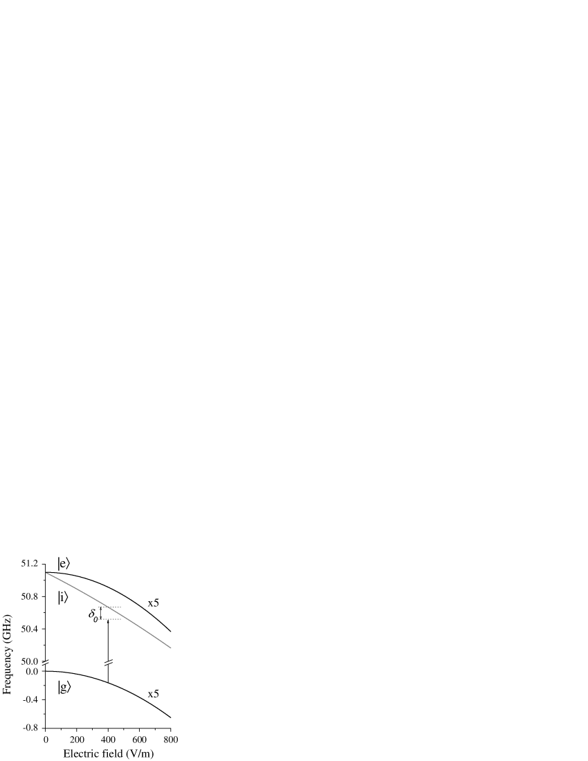
Figure 9: Energies of levels $|g\rangle$, $|e\rangle$ and $|i\rangle$ as a function of the electric field. States $|g\rangle$ and $|e\rangle$ have a small, approximately quadratic Stark effect, magnified in this figure by a factor 5 for the sake of clarity. Level $|i\rangle$ has a much larger, linear Stark effect. The microwave dressing (vertical arrow) predominantly mixes $|g\rangle$ and $|i\rangle$ and reduces the difference in Stark polarizability between $|e\rangle$ and $|\widetilde{g}\rangle$, the resulting dressed level.

We note here that this scheme would also compensate for the problem of patch effects on the surface of the electrodes if the field which they create remains relatively small compared to the directing field amplitude $E_{a}$. This effect is caused by the misalignment of crystal orientation in adjacent crystals in the metal. Let us consider a surface with voltage difference $\Delta V$ between adjacent crystals of characteristic size $a$. An ensemble of such patches will create at a distance $d$ above the surface a field:

$$E_{\mbox{\tiny patch}}=\frac{a\Delta V}{d^{2}}.$$ (30)

Over a volume of dimension $\Delta r$, this field has an inhomogeneity of the order of:

$$\Delta E_{\mbox{\tiny patch}}=\frac{a\Delta V\Delta r}{d^{3}}.$$ (31)

Patch-effects for Gold electrodes were measured at much closer distances in Ref. QC_YALESHIFTS96 where they found $E_{\mbox{\tiny patch}}\simeq 10^{4}$ V/m for $d=0.25\ \mu$m and $a\simeq 30$ nm. Being conservative, we assume the patch size to be 100 nm. Building on these figures we estimate the field to be $0.008\pm 0.0003$ V/m for trap A and $0.15\pm 0.005$ V/m for trap B, the inhomogeneity being calculated over a volume of dimension $\Delta r=15\ \mu$m and 5 $\mu$m, the typical excursion of atoms in traps A and B respectively. All of these values remain much smaller than $E_{a}$ and would hence be well compensated for by our technique.

5.3 Assessment of performances

The simple explanation of Sec. 5.2 is, however, far from describing the true physical reality:

• The value calculated for $\delta_{0}$ is not significantly smaller than the energy difference between state $|i\rangle$ and state $|i^{\prime}\rangle$ (see Fig. 1), which is therefore also significantly coupled to $|g\rangle$. Moreover the microwave field also couples state $|e\rangle$ to the $n=52$ manifold. It is therefore important to adopt a multilevel approach in order to account for the coupling by the $\pi$-polarized dressing microwave of all the levels of equal $m$ (see Fig. 1).

• This coupling therefore mixes the level $|g\rangle$ with other levels of the same $m=49$ (as is its aim) and equally $|e\rangle$ with levels of $m=50$. It must not be forgotten, however, that these levels have finite, potentially short, lifetimes in the cavity. We can therefore now see a form of spontaneous emission by $|\widetilde{g}\rangle$ and $|\widetilde{e}\rangle$ in which they absorb a photon from the dressing microwave mode and immediately re-emit it into another mode of the cavity. These spontaneous events would destroy any coherence existing between $|\widetilde{g}\rangle$ and $|\widetilde{e}\rangle$. We must therefore quantify the rate at which these events occur and check that the corresponding lifetime is not limiting.

• The dressed level transition frequency $\omega_{e\tilde{g}}$ is dramatically dependent on the microwave Rabi frequency, previously considered constant and equal to $\Omega_{0}$. But $\Omega$ is actually time- and position-dependent due to the spatial profile of the mode (nodes at $y=\pm 1$ cm, see Sec. 5.2) and due to the variation of $\theta(\vec{r},t)$. The instantaneous Rabi frequency experienced by an atom is therefore given by $\Omega(\vec{r},t)=\Omega_{0}f(\vec{r})\cos\theta(\vec{r},t)$. This variation of the Rabi frequency creates an inhomogeneous broadening which must be included in our final calculation.

• The tilt $\theta$ also couples a fraction of the microwave power to $\sigma$ transitions within the Rydberg levels, with an effective Rabi frequency $\Omega_{\sigma}(\vec{r},t)\propto\Omega_{0}f(\vec{r})\sin\theta(\vec{r},t)$, significantly smaller than $\Omega$. The large detuning $\delta_{0}$ prevents us from having resonant one-photon transitions between the levels $|e\rangle$ and $|g\rangle$ due to this coupling. Nevertheless, there could exist a multiphoton transition coupling the circular states to adjacent manifolds. A 1 Hz Rabi frequency would be sufficient to transfer population from the circular state to this adjacent one, and limit the coherence time between $|e\rangle$ and $|\widetilde{g}\rangle$ to 1 s. We must therefore check that no such resonance exists.

• To achieve the necessary precision in the position of the levels $|e\rangle$, $|g\rangle$, $|i\rangle$ and $|i^{\prime}\rangle$ we must go beyond the quadratic Stark expansion of Eq. 1.

We will now address these points one by one, turning first of all to the last. To achieve the precision necessary we diagonalize the Stark Hamiltonian of the circular state and the 4 manifolds of greater $n$ above it, in the presence of an electric field. The resulting energies were fitted by a 4th order polynomial over electric fields from 0 to 1000 V/m with an error less than 0.5 Hz. It was checked that adding a 5th manifold above the circular state to the Hamiltonian changed the resulting energies by less than 1 Hz.

In order to take account of the coupling of levels other than $|g\rangle$ and $|i\rangle$ by the microwave field, we must carry out a diagonalization of a Hamiltonian containing all relevant couplings. The microwave field is fully defined by its classical Rabi frequency at trap centre $\Omega_{0}$ on the $|g\rangle\rightarrow|i\rangle$ transition and its detuning $\delta_{0}$. The angle $\theta(\vec{r},t)$ being small, we consider firstly only the $\pi$-polarized component of the microwave field, coupling levels of equal $m$. We have adopted a dressed level approach to this problem and therefore consider the ladder of levels $|n,n_{1},m,n_{\pi}\rangle$ where the additional quantum number $n_{\pi}$ counts the number of photons in the microwave field. For the case $m=49$, relevant for level $|g\rangle$, the coupling between initial and final states $|n_{i},n_{1,i},49,n_{\pi}+1\rangle$ and $|n_{f},n_{1,f},49,n_{\pi}\rangle$ is given by:

$$\Omega_{n_{i},n_{1,i}}^{n_{f},n_{1,f}}(n_{\pi})=\Upsilon_{n_{i},n_{1,i}}^{n_{f},n_{1,f}}\sqrt{n_{\pi}+1}$$ (32)

where $\Upsilon_{n_{i},n_{1,i}}^{n_{f},n_{1,f}}$ is the Rabi frequency on the considered transition for $n_{\pi}=0$, proportional to the dipole matrix element $\mathcal{M}_{n_{i},n_{1,i}}^{n_{f},n_{1,f}}$. However, as the dressing microwave is a classical field (and hence $n_{\pi}\gg 1$), one can assume $\sqrt{n_{\pi}}\approx\sqrt{n_{\pi}+1}\approx\mbox{constant}$. Therefore each coupling strength can be normalized to $\Omega_{0}$ according to:

$$\Omega_{n_{i},n_{1,i}}^{n_{f},n_{1,f}}(n_{\pi})=\Omega_{0}\frac{\Upsilon_{n_{i},n_{1,i}}^{n_{f},n_{1,f}}}{\Upsilon_{50,0}^{51,1}}=\Omega_{0}\frac{\mathcal{M}_{n_{i},n_{1,i}}^{n_{f},n_{1,f}}}{\mathcal{M}_{50,0}^{51,1}}.$$ (33)

We were therefore able to construct the matrix of a Hamiltonian at constant $m$ including $M$ multiplicities in $n$ (ie. $n=m+1,\cdots,m+M$), and $2N+1$ multiplicities in $n_{\pi}$ (ie. $n_{\pi}-N,\cdots,n_{\pi},\cdots,n_{\pi}+N$). For the initial level positions $\mathcal{E}(k;E)$ we use the quadratic Stark expansion of Eq. 1 for all levels apart from $|g\rangle$, $|e\rangle$, $|i\rangle$ and $|i^{\prime}\rangle$, as explained above. After diagonalization of this Hamiltonian, we are left with a new ladder of levels, $\widetilde{\mathcal{E}}(k;E)$. These levels are slightly shifted in energy with respect to the unperturbed states and it is of course this shift that we hope to use in order to render $\widetilde{\mathcal{E}}(g,n_{\pi};E)$ and $\widetilde{\mathcal{E}}(e,n_{\pi};E)$ parallel. This shift being small, and there being no resonant coupling due to the dressing field, we are able to associate each of the dressed levels unambiguously with one of the unperturbed levels. We label the state arising from $|n,n_{1},m,n_{\pi}\rangle$ as $\widetilde{|n,n_{1},m,n_{\pi}\rangle}$ where the new quantum numbers characterize the now mixed atom-field state. We computed the change in energy of $\widetilde{\mathcal{E}}(g,n_{\pi};E)$ and $\widetilde{\mathcal{E}}(e,n_{\pi};E)$ as one increases $M$ or $N$ by one, hence increasing the size of the Hamiltonian diagonalized. We found this difference to decrease exponentially and fall below the Hz level for $M\geq 6$ and $N\geq 4$. By a diagonalization of the Hamiltonian with $M=6$ and $N=4$ we were therefore able to calculate $\widetilde{\mathcal{E}}(g,n_{\pi};E)$ and $\widetilde{\mathcal{E}}(e,n_{\pi};E)$ to the Hz level for a given electric field $E$, microwave power (corresponding Rabi frequency $\Omega_{0}$) and detuning $\delta_{0}$. We can therefore write:

$$\mathcal{E}_{k}(E,\Omega_{0},\delta_{0})=\widetilde{\mathcal{E}}(k,n_{\pi};E)-n_{\pi}\hbar\omega_{0},$$ (34)

for the potential energy of a trapped atom in state $k=g$ or $e$, in the presence of the microwave dressing field.

From these energies one can determine the dressed level transition frequency:

$$\omega_{\tilde{e}\tilde{g}}(E,\Omega_{0},\delta_{0})=\left[\mathcal{E}_{e}(E,\Omega_{0},\delta_{0})-\mathcal{E}_{g}(E,\Omega_{0},\delta_{0})\right]/\hbar,$$ (35)

and analyse its dependence on the electric field. In the neighbourhood of $E_{a}$ we have:

$$\omega_{\tilde{e}\tilde{g}}(E,\Omega_{0},\delta_{0}) = \omega_{\tilde{e}\tilde{g}}(E_{a},\Omega_{0},\delta_{0})$$

$$+L(E_{a},\Omega_{0},\delta_{0})(E-E_{a})$$

$$+Q(E_{a},\Omega_{0},\delta_{0})(E-E_{a})^{2}$$

$$+O((E-E_{a})^{3}),$$

and it is the coefficients $L(E_{a},\Omega_{0},\delta_{0})$ and $Q(E_{a},\Omega_{0},\delta_{0})$ that we hope to cancel, as we did under the simpler, two-level treatment laid out in Sec. 5.2. Unfortunately, due to the effect of the microwave field upon level $|e\rangle$ as well as $|g\rangle$, we find that, while it is possible for any $\delta_{0}$ to find an $\Omega_{0}$ such that $L(E_{a},\Omega_{0},\delta_{0})=0$, it remains nonetheless impossible to simultaneously cancel $Q(E_{a},\Omega_{0},\delta_{0})$. We therefore content ourselves with canceling $L(E_{a},\Omega_{0},\delta_{0})$ and bringing $Q(E_{a},\Omega_{0},\delta_{0})$ close to its minimum for the reasonable parameter values $\Omega_{0}=2\pi\times 200.000$ MHz and $\delta_{0}=2\pi\times 555.907$ MHz. The remaining frequency dispersion corresponding to the field excursion $\Delta E=1$ V/m is of the order of 10 Hz.

Turning now to the second item on our list of imperfections in the simplistic treatment of Sec. 5.2, we must analyse the effect of the variation of $\Omega(\vec{r},t)$ due to the mode profile, the angle $\theta(\vec{r},t)$ or, indeed, simple technical noise on the microwave amplifier. By analysing the variation of $\omega_{\tilde{e}\tilde{g}}(E_{a},\Omega_{0}+\Delta\Omega,\delta_{0})$ with $\Delta\Omega$ we were able to determine that the consequent inhomogeneous broadening is less than $10$ Hz for $\Delta\Omega/\Omega<2\times 10^{-7}$. This sets a tight condition on the power stability of the microwave source for the dressing. Both the excursion of the atom in the microwave field profile and the variation of $\theta(\vec{r},t)$ introduce a $\Delta\Omega$ smaller than this.

The rate of spontaneous cascades of the type $\widetilde{|g,n_{\pi}\rangle}\rightarrow\widetilde{|k,n_{\pi}-1\rangle}$ is found by calculating the dipole $\vec{D}(\widetilde{g}\widetilde{k})$ between $\widetilde{|g,n_{\pi}\rangle}$ and all the eigenstates $\widetilde{|k,n_{\pi}^{\prime}\rangle}$ of lower energy and then summing the rates of spontaneous transitions, proportional to the square of the dipole. The lifetimes thus calculated converge rapidly with increasing $M$ and $N$ towards 11.9 s for $|\widetilde{g},\widetilde{n_{\pi}}\rangle$ and 62.0 s for $|\widetilde{e},\widetilde{n_{\pi}}\rangle$ (much longer because of the greater detuning of the microwave for transitions within the $m=50$ multiplicity and the consequently smaller contamination of $|e\rangle$ by other levels). These lifetimes are much longer than those already imposed by other limitations as presented in Sec. 4.2 and are therefore not an obstacle.

Finally, it was checked that there were no resonances between the dressed circular states and adjacent levels of different $m$ due to the small $\sigma$-polarized component of the microwave field. No transition was found towards the multiplicities of $\Delta m=\pm\ 1$ with a detuning of less than 100 MHz. These transitions consequently pose no problem. All transitions at $\Delta m=\pm\ 2,3\ldots$ have Rabi frequencies $\ll 1$ Hz, these processes being of second or higher order, passing necessarily by a virtual transition at $\Delta m=\pm\ 1$ which we have just seen to be hugely nonresonant, and hence strongly suppressed.

5.4 Simulation of the coherence control

In order to estimate the coherence decay time $T_{2}$ we simulated a Ramsey interferometry experiment in the presence of the dressing microwave. We simulate the trajectories of an atom as in Sec. 2.4 with the state dependent potential energy given by:

$$\mathcal{E}_{k}(\vec{r},t)=\overline{\mathcal{E}}_{k}(E(\vec{r},t),\Omega_{0}f(\vec{r})\cos\theta(\vec{r},t),\delta_{0}),$$ (37)

where the $\overline{\mathcal{E}}_{k}(E,\Omega,\delta)$ is a series expansion of the $\mathcal{E}_{k}$ to fourth order in $E$ and $\Omega$ around $(E_{a},\Omega_{0},\delta_{0})$. $E(\vec{r},t)$ and $\theta(\vec{r},t)$ are the electric field amplitude and tilt, and $f(\vec{r})$ accounts for the dressing microwave spatial mode (see Sec. 5.2).

Figure 10: Phase acquired by an $|\widetilde{e}\rangle/|\widetilde{g}\rangle$ coherence over 40 ms. The trajectory considered is in trap A, under the conditions of Table 3 and at $T_{0}=300$ nK.

We assume that the atom undergoes two short microwave $\pi/2$ pulses, resonant on the $|\widetilde{g}\rangle/|\widetilde{e}\rangle$ transition (frequency $\omega_{\tilde{e}\tilde{g}}(E_{a},\Omega_{0},\delta_{0})$) at times $t_{i}$ and $t_{f}$, separated by a long delay $T=t_{f}-t_{i}$. For each state we follow the state dependent trajectory. For atoms taken from a sample at $0.3\ \mu$K, the average separation between the two is $\sim 20$ nm, much smaller than the de Broglie wavelength $\lambda_{DB}=0.34\ \mu$m. The Stern Gerlach effect can therefore be neglected. The dephasing between the two states is then due only to the phase $\phi(T)$ acquired by the $|\widetilde{e}\rangle/|\widetilde{g}\rangle$ coherence along the trajectory $\vec{r}(t)$:

$$\phi(T) =\int_{t_{i}}^{t_{f}}\left[\right. \overline{\mathcal{E}}_{e}(E\left[\vec{r}(t),t\right],\Omega_{0}f\left[\vec{r}(t)\right]\cos\theta\left[\vec{r}(t),t\right],\delta_{0})$$ (38)

$$-\overline{\mathcal{E}}_{g}(E\left[\vec{r}(t),t\right],\Omega_{0}f\left[\vec{r}(t)\right]\cos\theta\left[\vec{r}(t),t\right],\delta_{0})$$

$$\left.-\omega_{\tilde{e}\tilde{g}}(E_{a},\Omega_{0},\delta_{0})\ \right]dt.$$

Fig. 10 represents this phase evolution for a given trajectory over a 40 ms time interval. One can see that, over times longer than the trap oscillation period, the evolution is quite linear. On times scales of the order of the trap period, $\phi(T)$ proceeds by small steps of amplitude $\Delta\phi$ which occur when the atom is furthest from the origin. The final fringe contrast for the whole set of trajectories can be evaluated by $C=(\overline{\cos\phi}^{2}+\overline{\sin\phi}^{2})^{1/2}$ (where the bar denotes an average over all trajectories). The time evolution of $C$, shown in Fig. 11(a), provides an estimate of $T_{2}$ at around 25 ms. This is in qualitative agreement with the predictions of Sec. 5.3. The evolution of the contrast over long time is, however, nonexponential. After a very rapid initial fall, $C(T)$ decays at a much slower rate. We attribute this behaviour to the fraction of trajectories which remain very close to the center of the trap and whose phase drift can be much smaller than 1 over significantly long times [see Fig. 11(b)].

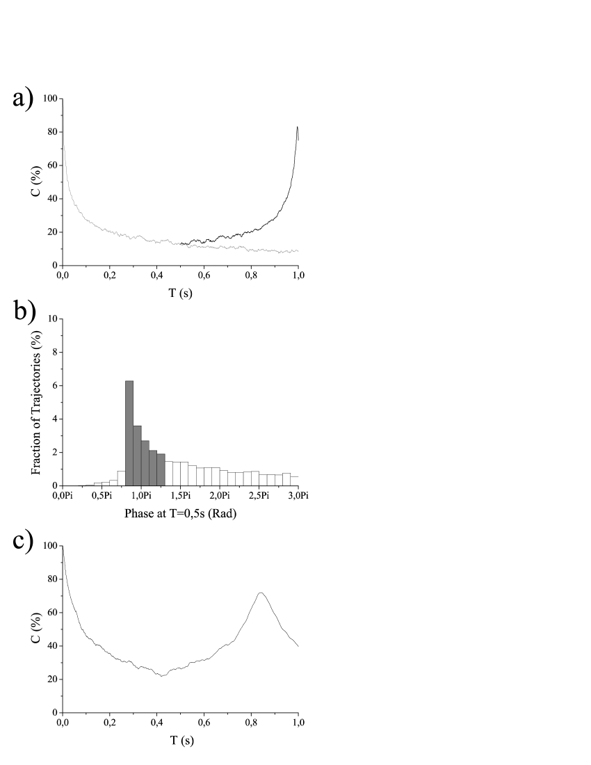
Figure 11: (a) Simulated Ramsey fringe contrast $C$ as a function of the time interval $T$ between two $\pi/2$ pulses in the case of Trap A. Conditions are as in Table 3 with $T_{0}=300$ nK, we average over 10000 trajectories. Grey line: contrast decay without echo. The contrast undergoes a non-exponential decay, falling to 50% in 24 ms, and to 13% in 0.5 s. Black line: contrast decay and then revival after a $\pi$-pulse at $T_{\pi}=0.5$ s, reaching 83% at $T=1$ s. (b) The histogram of the phases accumulated at $T$=0.5 s sheds light on this behaviour. A subset of the trajectories (white bars in the histogram) accumulates large phases and its contribution averages rapidly to zero. The other trajectories (grey bars), remaining closer to the centre of the trap, have a much slower phase drift and account for the slow decay at long times. (c) Simulated Ramsey fringe contrast $C(T)$ in Trap B under the conditions of Table 3 and with $T_{0}=300$ nK, averaged over 2500 trajectories. Here we have applied a $\pi$-pulse at $T=420$ ms and we see a revival of the contrast reaching 72% at $T=840$ ms.

As the phase acquired is almost perfectly linear with time for all trapped trajectories, one can try to combat the long term phase spreading using an echo technique reminiscent of photon-echo techniques. Coherence preserving echoes have also been tested for trapped ground-state atoms or ions TR_ECHODAVIDSON03 ; TR_ECHOBONN03 ; ION_WINELANDTRANSPORTION02 . In order to examine the efficiency of this technique we simulate, at a time $T_{\pi}$ after the first Ramsey pulse, an additional $\pi$-pulse on the $|\widetilde{e}\rangle/|\widetilde{g}\rangle$ transition, exchanging the populations of the two states. Pulse imperfections are taken into account for by considering, instead of a perfect $\pi$-pulse, a pulse performing the following transformation:

$$|\widetilde{g}\rangle \rightarrow \cos(\frac{\pi+\vartheta}{2})|\widetilde{g}\rangle+\sin(\frac{\pi+\vartheta}{2})|\widetilde{e}\rangle,$$ (39)

$$|\widetilde{e}\rangle \rightarrow -\sin(\frac{\pi+\vartheta}{2})|\widetilde{g}\rangle+\cos(\frac{\pi+\vartheta}{2})|\widetilde{e}\rangle.$$ (40)

where $\vartheta$ can be considered as the error in the angle of rotation in the Bloch sphere, $\vartheta=0$ corresponding to the ideal case. The $\vartheta$ for each trajectory is randomly chosen from a gaussian distribution, centered around $0$, with a dispersion of 0.1 Rad. In the ideal case where $\vartheta=0$ the phase of the $|\widetilde{e}\rangle/|\widetilde{g}\rangle$ coherence is multiplied by -1 upon application of the $\pi$-pulse. During the subsequent evolution, the phase drift continues as before and thus returns towards zero. At time $T=2T_{\pi}$, all phases are zero to within an uncertainty of the order of the average phase step amplitude $\Delta\phi$.

Fig. 11(a) also presents the contrast $C$ obtained under these conditions as a function of $T$ with a $\pi$-pulse applied at $T_{\pi}=0.5$ s. We see it increase sharply up to 83% around $T=2T_{\pi}=1$ s. This very high contrast corresponds to an effective $T_{2}=5.4$ s. Even for atoms at $T_{0}=1\ \mu$K, we obtain $C(2T_{\pi})=$57.3%. Fig. 11(c) shows that the technique also works in trap B, producing an effective $T_{2}$ of 2.6 s. More complex echo sequences can be envisaged to improve the final Ramsey fringe contrast. Ideal $\pi$-pulses repeated at shorter time intervals can maintain the coherence over time scales in the minute range, being only limited by the radiative lifetime.

6 Conclusions and perspectives

We have shown that it is possible to integrate on a microchip the elements necessary to excite a single atom into a circular Rydberg state, to trap it, and to perform coherent manipulation of its internal states over seconds. The wealth of possible electrode geometries makes it easy to extend these results to the case of atomic waveguides or arrays of traps. We have also obtained preliminary results proving that it could be possible to integrate the detection of the Rydberg states on the chip itself. This relies on the usual state dependent field ionization of the atom followed by detection of the electron by a thin superconducting wire, such as those already used in fast photon detectors SEMENOVREVIEW_02 . Our proposal would offer a complete “toolbox” to study and control a single quantum system in an extremely versatile manner. It also forms a scalable architecture for quantum information processing. The experimental realization of this project will require the adaptation of atom-chip techniques from room temperature to the superconducting regime. We are currently developing a cryogenic experiment able to achieve this, opening new perspectives for atom-chip experiments.

- (1) T. D. Ladd, D. Maryenko, Y. Yamamoto, E. Abe, K. M. Itoh Phys. Rev. B 71, 014401 (2005)
- (2) D. Vion, A. Aassime, A. Cottet, P. Joyez, H. Pothier, C. Urbina, D. Esteve, M. Devoret Science 296, 886 (2002)
- (3) Y. Nakamura, Y. A. Pashkin, T. Yamamoto, J. S. Tsai Phys. Rev. Lett. 88, 047901 (2002)
- (4) M. H. Anderson, J. R. Ensher, M. R. Matthews, C. E. Wieman, E. A. Cornell Science 269, 198 (1995)
- (5) B. DeMarco, D. S. Jin Science 285, 1703 (1999)
- (6) J. Denschlag, D. Cassetari, A. Chenet, S. Schneider, J. Schmiedmayer Appl. Phys. B 69, 291 (1999)
- (7) J. Reichel, W. Hänsel, T. W. Hänsch Phys. Rev. Lett. 83, 3398 (1999)
- (8) J.-M. Raimond, M. Brune, S. Haroche Rev. Mod. Phys. 73, 565 (2001)
- (9) M. Brune, E. Hagley, J. Dreyer, X. Maître, A. Maali, C. Wunderlich, J.-M. Raimond, S. Haroche Phys. Rev. Lett. 77, 4887 (1996)
- (10) A. Rauschenbeutel, G. Nogues, S. Osnaghi, P. Bertet, M. Brune, J.-M. Raimond, S. Haroche Science 288, 2024 (2000)
- (11) I. E. Protsenko, G. Reymond, N. Schlosser, P. Grangier Phys. Rev. A 65, 052301 (2002)
- (12) P. Hyafil, J. Mozley, A. Perrin, J. Tailleur, G. Nogues, M. Brune, J. M. Raimond, S. Haroche Phys. Rev. Lett. 93, 103001 (2004)
- (13) M. Lukin, M. Fleischhauer, R. Côté, L. Duan, D. Jacksch, J. Cirac, P. Zoller Phys. Rev. Lett. 87, 037901 (2001)
- (14) S. K. Dutta, J. R. Guest, D. Feldbaum, A. Walz-Flannigan, G. Raithel Phys. Rev. Lett. 85, 5551 (2000)
- (15) T. Gallagher Rydberg atoms (Cambridge University Press, Cambridge) (1994)
- (16) M. Gross, J. Liang Phys. Rev. Lett. 57, 3160 (1986)
- (17) W. Paul Rev. Mod. Phys. page 531 (1990)
- (18) E. Peik Eur. Phys. J. D 6, 179 (1999)
- (19) Scientific Instrument Services Inc. www.simion.com SIMION 3D, Ion Modeling Software
- (20) M. Saffman, T. G. Walker Phys. Rev. A 66, 065403 (2002)
- (21) R. Folman, P. Krueger, J. Schmiedmayer, J. Denschlag, C. Henkel Adv. At. Mol. Opt. Phys. 48, 263 (2002)
- (22) W. Hänsel, J. Reichel, T. Hänsch Phys. Rev. Lett. 86, 608 (2001)
- (23) W. Hänsel, P. Hommelhoff, T. W. Hänsch, J. Reichel Nature (London) 413, 498 (2001)
- (24) S. Groth, P. Kruger, S. Wildermuth, R. Folman, T. Fernholz, J. Schmiedmayer, D. Mahalu, I. Bar-Joseph Appl. Phys. Lett. 85, 2980 (2004)
- (25) P. Nussenzveig, F. Bernardot, M. Brune, J. Hare, J.-M. Raimond, S. Haroche, W. Gawlik Phys. Rev. A 48, 3991 (1993)
- (26) S. Haroche in Fundamental Systems in Quantum Optics, Les Houches Summer School, Session LIII, edited by J. Dalibard, J.-M. Raimond, J. Zinn-Justin (North Holland, Amsterdam) page 767 (1992)
- (27) R. G. Hulet, E. S. Hilfer, D. Kleppner Phys. Rev. Lett. 55, 2137 (1985)
- (28) W. Jhe, A. Anderson, E. A. Hinds, D. Meschede, L. Moi, S. Haroche Phys. Rev. Lett. 58, 666 (1987)
- (29) J. D. Jackson Classical electrodynamics (Wiley, New York) second edition (1975)
- (30) H. Katori, M. Takamoto Phys. Rev. A 66, 065403 (2002)
- (31) D. M. Harber, H. J. Lewandowski, J. M. McGuirk, E. A. Cornell Phys. Rev. A 66, 053616 (2002)
- (32) P. Treutlein, P. Hommelhoff, T. Steinmetz, T. W. Hänsch, J. Reichel Phys. Rev. Lett. 92, 203005 (2004)
- (33) V. Sandoghdar, C. Sukenik, S. Haroche, E. Hinds Phys. Rev. A 53, 1919 (1996)
- (34) M. F. Andersen, A. Kaplan, N. Davidson Phys. Rev. Lett. 90, 023001 (2003)
- (35) S. Kuhr, W. Alt, D. Schrader, I. Dotsenko, Y. Miroshnychenko, W.Rosenfeld, M. Khudaverdyan, V. Gomer, A. Rauschenbeutel, D. Meschede Phys. Rev. Lett. 91, 213002 (2003)
- (36) M. Rowe, A. Ben-Kish, B. DeMarco, D. Leibfried, V. Meyer, J. Beall, J. Britton, J. Hughes, W. M. Itano, B. Jelenkovic, C. Langer, T. R. D. J. Wineland Quantum Inf. Comp. 2, 257 (2002)
- (37) A. D. Semenov, G. Gol’tsman, R. Sobolewski Supercond. Sci. Technol. 15, R1 (2002)