Аннотация

In this paper we discuss analogue computers based on quantum optical systems accelerating dynamic programming for some computational problems. These computers, at least in principle, can be realized by actually existing devices. We estimate an acceleration in resolving of some NP-hard problems that can be obtained in such a way versus deterministic computers.

Key words: analogue quantum machine, complexity theory, dynamic programming

1 Introduction

Quantum computing is intensive developing intersection of physics and informatics since (Feynman 1982; Shor 1994; Grover 1997; Preskill 1998). But schemes of universal quantum computers working by qubits meet formidable difficulties in their realization as real physical devices (Dyakonov 2003). In this note we develop another approach based on analogue realization of quantum computing. We concentrate our attention on some particular NP-hard problems. For a given problem we can try to construct a quantum analogue machine that resolves this problem by means of time evolution.

Recall (Garey and Johnson 1979) that, roughly speaking, a problem with instances $I$ lies in the class NP if there is a polynomial time $P(|I|)$ algorithm checking a solution (if this solution is provided) where $|I|$ is the size of the input $I$. The problem is NP-hard if $P=NP$ whenever this problem belongs to $P$. The list of NP-complete problems contains many important problems of number theory, graph theory, logic etc. Some of the most known NP-complete problems are travelling salesman problem, satisfiability, knapsack, matrix cover etc. (see a list in (Garey and Johnson 1979)). Let us observe that all the NP-complete problems, are, in a sense, polynomially equivalent. This means that there are polynomial time reductions between different problems.

An analogue quantum machine or resolving of combinatorial search NP-hard problems has been proposed by (Farhi et al. 2000). Let us consider 3-SAT problem in which we deal with a family of $N$ clauses of the form $(B_{i_{1}}\ \bigvee\ B_{i_{2}}\ \bigvee\ \neg\ B_{i_{3}})$ or $(B_{i_{1}}\ \bigvee\ \neg\ B_{i_{2}}\ \bigvee\ \neg\ B_{i_{3}})$ or $(B_{i_{1}}\ \bigvee\ B_{i_{2}}\ \bigvee\ B_{i_{3}})$ etc., where $B_{j}$ are boolean variables taking values True or False. The problem is whether one can assign such values to all the variables that all the clauses will become true.

The approach of (Farhi et al. 2000) uses quantum adiabatic theorem. The authors describe a formal Hamiltonian such that its ground state gives us a solution of 3-SAT problem. The bound of the actual speed-up yielded by this algorithm depends on the spectral gap between the ground state and the first excited state. If this gap is exponentially small the time of solving is exponentially large. It is a very difficult problem to estimate the value of this gap and thus it is not easy to show, in general, that such an algorithm really gives a quantum acceleration. (Another NP-complete problem that can be naturally associated with a Hamiltonian is the problem of minimization of energy of spin glass with a large number of spins (see (Garey and Johnson 1979, p. 282.))

The second difficulty with such approach is that it is not obvious to realize physically qubits and Hamiltonian with very nonlocal nontrivial interaction between qubits. It seems that difficulties in physical realization of Feynman quantum computers or analogue computers from (Farhi et al. 2000) are significant and some authors even believe (see, for example, (Dyakonov 2003)) that such computers are physically non-realizable.

The approach of (Farhi et al. 2000) uses a specific structure of 3-SAT problem. If we use some universal approach that does not take into account a specific form of the problem, we can expect a quantum acceleration in time ${N}^{1/2}$ (Grover 1997), i.e., if a deterministic computer makes a search in $N$ steps then quantum universal computers will make the same search in $N^{1/2}$ steps. Further, it was shown that acceleration, with a universal approach can be achieved by at most $N^{1/6}$ Beals et al. 1998; Preskill 1998. Notice that this quantum $N^{1/2}$ acceleration is less than an acceleration that can be obtained by special deterministic and probabilistic algorithms with respect to trivial exhaustive search (Dantsin et al. 2003). Once more quantum machine based on quantum optics phenomena was discussed in (Kazakov 2003). The earlier analogue computational machines were discussed in (Matiyasevich 1987; Blass 1989).

In this paper we describe a quantum machine which, as we believe, can be realized physically and which may accelerate solving of some NP-complete problems. Our machine uses different linear and nonlinear quantum optical devices that can be constructed actually and, thus, our computer, at least in principle, can be practically realized. An acceleration that can be obtained heavily depends on different characteristics of our devices. We estimate this acceleration vs. deterministic computers using the characteristics of actually existing devices.

2 Statement of problems. Known results.

We consider the following problems which are NP-hard (Papadimotriou, Steiglitz 1982; Garey, Johnson 1979).

1 Boolean knapsack, variant 1

Given positive integers $c_{j}$, $j=1,...n$ and $K$, is there a subset $S$ of $\{0,1,...,n\}$ such that $\sum_{j\in S}c_{j}=K$?

In other words, whether there exist $n$ boolean values $s_{i}\in\{0,1\}$ such that $\sum_{i=1}^{n}c_{i}s_{i}=K?$

Here the size $|I|$ of the instance $\{n,c_{1},c_{2},...,c_{n},K\}$ is the number of bits needed for binary representations of all the integers $c_{i},K$. We can suppose, without loss of generality that $c_{i}<K$. Thus, size $|I|$ can be estimated roughly as $O(n\log K)$.

2 Boolean knapsack, variant 2

Given integers $c_{j}$, $j=1,...n$ and $B_{-},B_{+}$, whether there exist $n$ boolean values $s_{i}\in\{0,1\}$ such that $\sum_{i=1}^{n}c_{i}s_{i}$ lies in the interval $(B_{-},B_{+})$? Here the instance size is roughly $O(n\log B_{+})$.

3 Optimization boolean knapsack

Given integers $c_{j}$ and $w_{i}$ , $j=1,...n$ and the number $B_{+}$, maximize the cost

$$\sum_{i=1}^{n}w_{i}s_{i}$$ (1)

defined by $n$ boolean variables $s_{i}\in\{0,1\}$ under condition that

$$\sum_{i=1}^{n}c_{i}s_{i}<B_{+}.$$ (2)

There is an important difference between the problems 1, 2 and 3. The output in 1,2 is "YES"or "NO". The output of 3 is a number, and one could try to approximate it.

Let us remind now some known results about 1, 2 and 3.

a All the problems 1-3 can be resolved by exhaustive search in $2^{n}$ steps.

b If $2^{n}>K$ then the problem 1 can be resolved by a more effective method, namely, by dynamic programming, in $O(nK)$ steps. This method can be described briefly as follows (for details, see Papadimotriou and Steiglitz 1982). The algorithm produces consecutively $\Sigma_{0},\Sigma_{1},...,\Sigma_{n}$ such that $\Sigma_{j}$ is the set of all possible subsums of $c_{1},...,c_{j}$ At the first step we set $\Sigma_{0}=\{0\}$. At $j+1$-th step, we set $\Sigma_{j+1}=(\Sigma_{j}\cup(\Sigma_{j}+c_{j+1}))\cap\{0,...,K\}$. The problem has a solution if at the last $n$-th step $K\in\Sigma_{n}$.

In a similar way, we can resolve problem 2, it takes $O(nB_{+})$ steps, and problem 3, it takes $O(n\min(B_{+},R_{opt}))$ steps, where $R_{opt}$ denotes the maximum cost (1).

c Suppose we solve an approximative problem 3, namely, we seek for a number close to a maximal cost. This means that we give up accuracy in exchange for efficiency of our algorithm. To this end we can apply a truncation procedure removing the last $t$ digits from the binary representations of $w_{i}$ and $c_{i}$. Let $w_{m}$ be the largest $w_{i}$. Such a procedure leads to a cost $R_{appr}$ satifying the estimate (Papadimotriou and Steiglitz 1982; Ibarra and Kim 1975)

$$\frac{R_{opt}-R_{appr}}{R_{opt}}<\epsilon,\quad\epsilon=\frac{n2^{t}}{w_{m}}$$ (3)

The approximating algorithm runs in time $O(n^{4}\epsilon^{-1})$ (Papadimotriou and Steiglitz 1982; Ibarra and Kim 1975). Thus this problem has an approximative solution that can be found in a polynomial number of steps. Notice however, that there are many NP-complete problems that cannot be approximated in such a way, for example, travelling salesman problem (Garey and Johnson 1979; Papadimotriou and Steiglitz 1982).

3 Description of the quantum machines

Consider $n+1$ points $x_{0}<x_{1}<x_{2},...<x_{n}=x_{f}$ located along $x-$ axis in $(x,y)$ -plane. At the first point we set a laser, which generates a narrow beam. The diameter of this beam will be denoted by $d_{b}$, the wave length of the laser radiation will be denoted by $\lambda$. Typical values of these parameters are $d_{b}\sim 2\cdot 10^{-3}m,\ \lambda\sim 5\cdot 10^{-7}m$.

Here we describe an analogue quantum optical device (QOD) for the knapsack problems 1,2. Its possible scheme is presented on fig 1.

An input laser beam is splitted by $50\%$ mirror A1 to two separate beams running two different trajectories. The beam 1 then is shifted by a plane optical plate on the value $c_{1}\kappa$ in (vertical) z-direction, which is perpendicular to the plane of our picture (here $\kappa$ means the minimal shift). Then the beams are on the second mirror B1 and united result (which is a combination of shifted and non-shifted beams) goes through amplifier C1. We suppose that this amplifier has the characteristics presented on fig. 2.

After passage of $m$ mirrors the propagating light will contain beams shifted in z-direction at all possible distances $\sum_{i=1}^{m}c_{i}s_{i}\kappa$, where the values $s_{i}\in\{0,1\}$ depend on the trajectory of the beam. At the final point we measure intensity of outcoming light by a charge-coupled device (CCD). A CCD camera uses a small rectangular piece of silicon to receive incoming light. This silicon wafer is a solid state electronic component which has been micro-manufactured and segmented into an array of individual light-sensitive cells called "pixels". The pixel of the most common CCD has size only about $\delta_{p}\approx 10^{-7}m\approx 0.2\lambda$, it measures the intensity of light independently from other pixels. Note, that namely $50\%$ mirrors are genuine quantum components in our device (Feynman 1985).

We denote by $R_{M}$ the z-size of the separating mirrors (and amplifiers). The last parameter important for estimating of quality of our machine is an angular divergence $\alpha$ of the laser beam. A usual laser produces a beam having the angular divergence of order $\alpha\sim d_{b}/\lambda\sim 4\cdot 10^{-5}$.

Our machine is completely defined thus by the following parameters:

$$n,R_{M},L,\delta,Y_{min},Y_{max},\lambda,d_{b},\alpha,\kappa,c_{i}.$$

For the problem 3, we use the following ideas. In order to realize sums (1, 2) we have to modify scheme presented on fig 1. Namely, together with z-shifts we use the horizontal beam shift in an orthogonal direction $y$. Notice that a beam shifted in $y$-direction contains this shift propagating on different trajectories $L_{1}$ and $L_{2}$ (see fig. 3). It means that after successive z- and y-shifts, which the initial beam gets propagating from $x_{0}$ to $x_{n}$, one obtains the set of beams whose z- and y-shifts are different sums

$$\sum_{i=1}^{n}c_{i}s_{i},\quad\sum_{i=1}^{n}w_{i}s_{i},$$

in accordance with trajectories.

At the end of the device we set CCD which measure the plane distribution of the outcoming light with z-coordinates $z<B_{+}-\delta_{p}$, where $\delta_{p}$ is as it was mentioned above the typical pixel size.

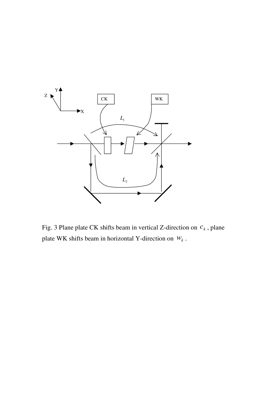
Рис. 1:

4 Solving the dynamic programming by the quantum optical device

Consider possible laser beam trajectories as a result of $n$ reflections on our mirrors. After the first series of reflections we obtain two beams running along lines $y=h_{1}$ and $y=0$ since each photon randomly chooses a way either along the first trajectories or the second one. So, the mirror system serves as a gate choosing the photon way. Remark that the mirror can be considered simultaneously as a quantum and a classical device. In a certain sense, our gates can be thus named as semiclassical quantum gates.

If we set a CCD that registrates photons at a point located after $x_{1}$, we could registrate two localized z-separated gaussian beams at $y=0$ and $y=H_{1}$.

So, in an ideal situation, QOD works as follows. Consider the problem 2. We set $H_{i}=\kappa c_{i}$, $i=1,2,...,n$, where $c_{i},n$ are given. We take now $Y_{min}=\kappa B_{-},\ Y_{max}=\kappa B_{+}$. Now turning on an input laser beam, we check, does the interval $(Y_{min},Y_{max})$ contain the center of the any laser beam (respectively, answer either "YES"or "

NO"). We suppose that CCD solves the problem with an error less than $1/3$.

It is not difficult to see that this method of solution can be considered as a physical realization of dynamic programming method from Section 2.

The problem 3 can be resolved approximatively, i.e., the global maximum can be estimated within some precision. However, to this end, we must modify slightly our consideration (see below).

Consider now diffraction effects. They can create an obstacle since one could registrate a photon not really passing correct gates as a photon that resolves our problem. In accordance with theory of gaussian beams (Svelto 1982) each gaussian beam has a finite transversal size and an angle of divergence $\alpha$. These values are connected by

$$\alpha\sim\frac{1.2\lambda}{d_{b}}.$$ (4)

After $n$ reflections, the size of an output beam becomes

$$d_{final}=nL\sin\alpha+d_{b},$$ (5)

where $L$ means distance between mirrors. Therefore, to get minimal value of $d_{final}$ we set

$$d_{b}=\sqrt{nL\lambda}.$$ (6)

Further, in order to separate on registering CCD the broadening gaussian beams (whose amplitude can differ up to factor 2 in accordance with fig.2), we have to restrict the minimal distance $\kappa$ between beams by

$$\kappa\geq d_{final}=2d_{b}.$$ (7)

In addition to (4.3) we have a geometric restriction

$$R_{M}>\kappa n+d_{b}.$$ (8)

This inequality means that the shifts of no beams jump out any mirrors.

One more problem is a possibility that, at some step $i=T_{0}$ many different beams arrive at the same point. It is not a mathematical difficulty (since this means the existence of many solutions) but it is a physical difficulty since it can lead to a high energy concentration and destruction of the mirrors. To avoid this effect we use active media that saturates the photon density (see fig. 2). This allows us to restrict the photon density at each point of the mirror by some constant.

Using of the active media leads however to new difficulty which can give us a lost of solutions. Namely, the phases of the photons of each beam become slightly different after passing the active media. Thus if the problem 2 has many solutions, CCD could not registrate any photons as a result of interference. This effect is possible if a phase shifts are significant. To overcome this difficulty we use special auto phase control devices known in optics. At the points $z_{1},z_{2},...z_{n}$ (see fig. 1) we places the phase-adjusting devices which measure phase of all beams and compare it with phase of a reference laser beam of the same frequency. Such adjustment gives the possibility to align phases of mixing beams.

5 Estimation of QOD performance for boolean knapsack

Let us estimate now what we can do using such a QOD and compare this machine performance with deterministic computer performance.

5.1 General estimates

There are three important parameters: a) the implementation cost; b) the energy cost of solving; c) the running time when we solve $M$ times the same problem with different inputs.

We compare here the dynamic programming for knapsack problems 1, 2 by a deterministic computer and by QOD. For the sake of unifying the notations we assume, that $B_{+}\leq K$.

For the QOD the implementation cost $CI_{quant}$ can be estimated roughly as

$$CI_{quant}=O(Kn)$$

since the mirror and amplifier sizes are of order $K$, the number of the mirrors and the cuvettes is $n$. The amplifier size is of order $Kn$, one can expect that energetical cost $CE_{qi}$ per one instance of the problem also is

$$CE_{qi}=O(Kn(n+K)),$$

where factor $n+K$ arises due to greatest length of the photon trajectory. The complete energy involved in $M$ calculations is then

$$CE_{quant}=O(Kn(n+K)M).$$

The implementation time has the order $Kn$ and the resolving time

$$Time_{quant}\ leC_{1}(n+K)M,$$

where $C_{1}$ is inverse proportional to the light speed and thus this coefficient is rather small. For the deterministic computer we have

$$CE_{det}=O(KnM),\quad Time_{det}=O(KnM)$$

Thus, QOD wins in time (taking into account both implementation and running times) vs. deterministic machine, while the order of consumed energy is higher than for a deterministic one.

5.2 Energetic and temporal costs

Our results include energetic and temporal costs of calculations. Let us consider a model, where this correspondence exhibits in a more explicit form. Let several polyhedra be placed in ${\bf R}^{3}$ and we have to calculate the length of the shortest path from the point A to the point B avoiding these polyhedra (treated as obstacles) (see fig.4). It is well known that this problem is NP-hard (Canny and Reif 1987). Moreover, even determining first $O(N^{1/2})$ bits of the length of the shortest path is NP-hard, where $N$ denotes the bits size of description of the instance of the problem (Canny and Reif 1987).

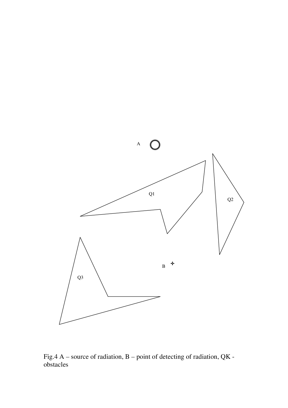
Рис. 2:

We can realize this calculation by the following analogue physical device. Let us place in the point A a source of radiation, in the point B - detector and polyhedral obstacles have mirror boundaries. If we turn the source A at initial moment $t=0$ and measure the time $t=t_{1}$ when our detector catches a first photon. Let the power of source be $J$ and frequency of radiation be $\nu$, then the number of created photons is $J/h\nu$, where $h$ is Planck’s constant (Karlov 1992). Each photon moves in its path and one can describe our analogue calculation as a "parallel computation"of the shortest path by different photons in which each photon plays the role of a processor.

In general, this first photon caught by the detector could not belong to the front wave (which corresponds to the shortest paths) due to a weakening of the wave and possible presence of the more strong waves. Therefore, increasing the intensity of the source allows to augment the probability to detect a photon of the wave front. So, we have to either repeat this experiment, with corresponding increasing of temporal cost, or increase the intensity of the source with increasing of energetic cost of calculation.

On the other hand, considered analogue devices have brought us to a conjecture that a tradeoff of the following kind

$$E\cdot T\geq Z,$$

holds, where $E$ and $T$ are energetical and temporal costs of this calculation respectively, and $Z$ depends on the problem. This means (at some extent) that there could be an "exchange"between the energy cost and the temporal cost needed to solve a computational task.

5.3 Estimates for real parameters

For the rate of a deterministic computer, for a single processor (we do not use a parallelism) we take the value $V=10^{10}operations/sec$. Suppose $2^{n}>B_{+}$, then the dynamic programming is more effective than the exhaustive search. Then a deterministic processor solves the problem 2 within time $T_{c}$

$$T_{c}\approx nB_{+}V^{-1}$$ (9)

Consider our optical processor. We see that $B_{+}$ must be subject to

$$B_{+}<R_{M}/\kappa.$$ (10)

Thus our possibilities are restricted by the mirror size. Then the problem can be resolved within time

$$T_{q}\approx(nL+R_{M})/c+nT_{atom},$$ (11)

where the second term describes the time when photons spend in the amplifier (which is at most $n$ times the relaxation time $T_{atom}$ for active atoms, $T_{atom}$ is about $10^{-8}sec$). The preprocessing (implementation) time for the optical machine is

$$T_{q,pre}\approx C_{2}Kn,$$

where $C_{2}$ is a constant.

It is interesting now to see what we could obtain by using really existing devices. As an example, we take the following typical parameter values:

$$R_{M}=nL=10m,\quad d_{b}=2\cdot 10^{-3}m,\quad\lambda=5\cdot 10^{-7}m.$$

Then $\kappa=5\cdot 10^{-3}m$ and $B_{+}<2\cdot 10^{2}$. For $n\geq 30$ the next inequality holds, $2^{n}>>nB_{+}$, and dynamic programming is more effective than the exhaustive search.

Minimal admissible difference $Y_{max}-Y_{min}$ can be estimated as $\kappa=5\cdot 10^{-3}m$. The deterministic time (5.1) is then $T_{det}\approx 30\cdot 2\cdot 10^{2}\cdot 10^{-10}\approx 10^{-6}sec.$ In accordance with (11) $T_{q}\approx 30/(3\cdot 10^{8})+30\cdot 10^{-8}\approx 10^{-6}sec.$

So, our conclusions for problem 1, 2 are the following. The performance of QOD is restricted by mirror sizes and beam diameter. The problem 2 can be solved by QOD and this effectiveness is essentially more vs. a deterministic processor if we repeat the same computation with different inputs many times. For realistic values of parameters, considered above, we can handle the case $n<60$, and then the speeds of the QOD and deterministic processor have the same order.

Let us discuss now situation for problem 3. In the next section we describe first modifications needed for resolving this problem. We will see that in this case the speed-up is much better.

6 Estimate of machine performance for optimization quantum knapsack

6.1 General estimates

We compare here the dynamic programming for knapsack problem 3 by a deterministic computer and by QOD using the parameters $CI$, $CE$, $Time$ described in Section 5.1.

For the quantum optical device the implementation (preprocessing) cost $CI_{quant}$ can be estimated roughly as

$$CI_{quant}=O(K^{2}n),$$

since the the mirror size is now of order $K^{2}$, the number of the mirrors is $n$. The amplifier takes volume of order $K^{2}n$, one can expect that the energetical cost $CE_{quant}$ is

$$CE_{quant}=O(K^{2}n(n+K)M),$$

where now $K$ majorates sums (1) and (2). However, if only numbers $w_{i}$ are large and $c_{i}\approx 1$, then the mirror area becomes again $O(K)$ as in Section 5, and we have the same estimates as in subsection 5.1.

One can estimate the resolving time

$$Time_{quant}=O((n+K)M).$$

For the deterministic computer we can (if we solve $M$ times the problem with different inputs) estimate energy similarly to 5.1 (problems 1,2)

$$CE_{det}=O(KnM),\quad Time_{det}=O(KnM).$$

Thus, if the number of inputs $M>>K$ then QOD has a chance to win, in time, with respect to a deterministic processor. The consumed energy of the QOD can be estimated by

$$CE_{quant}=O(K^{2}n(n+K)M)$$

(cf. subsection 5.1 above) whereas the energy consumed by a deterministic machine can be bounded again by $O(KnM)$ (cf. the discussion on the tradeoff of energy and time in subsection 5.1).

Let us consider now approximating solutions (see Section 2). Recall that the processing time of the deterministic processor in order to obtain an approximative solution, within precision $\epsilon$, is

$$Time_{det,appr}=O(Mn^{4}\epsilon^{-1}).$$

To compare this performance with effectiveness of our QOD, let us note that the pixel size is $\delta_{p}$ and thus the size of the mirrors in QOD solving the problem within relative precision $\epsilon$ should be $\delta_{p}/\epsilon=K\kappa$. Then the implementation cost will be

$$CI_{quant}=O((\delta_{p}/\epsilon\kappa)^{2}n),$$

resolving time can be estimated as $Time_{quant}=O((n+\delta_{p}/\epsilon\kappa)M)$ The choice $\delta_{p}$ is restricted by a small number of possible values, thus, $Time_{quant}+CI_{quant}$ grows in $n$ more slowly than $Time_{det,appr}$ for $\epsilon^{-1}=o(n^{3}M)$.

The consumed energy of QOD for approximating problem can be estimated by

$$CE_{quant,appr}=O((\delta_{p}/\epsilon\kappa)^{2}n(n+\delta_{p}/\epsilon\kappa)M)$$

which is less than the consumed energy for a deterministic machine (which is of the order $n^{4}\epsilon^{-1}M$) when $\epsilon^{-1}=o((n\kappa/\delta_{p})^{3/2})$.

6.2 Estimates for real device parameters

Recall that, to resolve the problem 3, we have modified QOD introducing additional parallel plates performing beam shifts in the direction $y$. So, we can suppose that $i$-th gate makes the shift to $H_{i}$ in the direction $z$ and to $H^{\prime}_{i}$ to the $y$ axis. As above, we set $H_{i}=\kappa c_{i}$ and $H_{i}^{\prime}=\kappa w_{i}$. At the end of the device we situate a set of CCD, which measure the intensity of light in $(y,z)$ plane.

Let us describe now how we can resolve, approximatively, any problem 3 without restrictions to the maximum of $B_{+}$. The key truncation idea can be found in (Ibarra and Kim 1975), see also (Papadimotriou and Steiglitz 1982). We reduce the case of arbitrary coefficients $c_{i}<B_{+},w_{i}$ to the previously studied case of restricted coefficients. To proceed it, we use the binary representations of these numbers. Suppose that each number use $\leq m$ the digits $0,1$, i.e. the size of the binary input is not much than $m$. Moreover, assume that the maximal admissible value of $B_{+}$ can be written down with only $m_{*}$ digits. Now we truncate each given number $c_{i},w_{i}$ and $B_{+}$ removing $m-m_{*}$ digits and allowing only first $m_{*}$ digits. With these new truncated data we can solve our problem and this solution gives an approximative solution.

The solving procedure to search an approximative solution of the problem 3 can be described as follows. We observe all beams that are measured by CCD and between them we choose a beam that have a maximal y-deviation. Such a scheme always gives an approximative solution of our problem, with precision of order $\kappa/2$.

Let us compare now a deterministic processor and QOD. Let us take the same parameters as above. The time processing for our device will be chosen the same as above, i.e., $T_{q}=10^{-6}sec$. For the deterministic computer, according to subsection 2c, one has

$$T_{c}\sim n^{4}V\epsilon^{-1},$$

where $\epsilon$ is the relative precision. The relative error of measurement we can estimate as $\epsilon\sim(\kappa/2)/R_{M}$, which corresponds to the separation of the gaussian beams with amplitudes differs by factor like 2. Substituting all the values in the last relation, we have $T_{c}\approx 1sec$, that much more than $T_{q}$. So, the quantum optical device gains an acceleration $10^{6}$ times vs a typical deterministic computer.

7 Conclusion

We have introduced and designed analogous quantum optical devices for simulating dynamic programming which provides the following complexity bounds (see notations in subsections 5.1, 6.1) for different versions of the knapsack problem (section 2).

Proposition 7.1.

i) For the versions 1,2 the implementation cost $CI_{quant}=O(Kn)$, the running time $Time_{quant}=O((n+K)M)$, and the energy cost $CE_{quant}=O(Kn(n+K)M)$;

ii) For the version 3 $CI_{quant}=O(K^{2}n)$, the running time $Time_{quant}=O((n+K)M)$, and the energy cost $CE_{quant}=O(K^{2}n(n+K)M)$;

iii) for $\epsilon$-approximative solution of the version 3 $CI_{quant}=O(n(\delta_{p}/\epsilon)^{2})$, the running time $Time_{quant}=O((n+\delta_{p}/\epsilon)M)$, and the energy cost $CE_{quant}=O(n(n+\delta/\epsilon)(\delta_{p}/\epsilon)^{2}M)$; (see subsections 5.1 and 6.1)

Also we compare these bounds with ones for deterministic machines (see subsections 5.1, 6.1).

Let us discuss briefly the "quantum properties"of QOD. The genuine quantum machine has to exploit two quantum properties: i) "exponential resource"connected with exponentially large dimension of the state space, and ii ) the "quantum parallelism"which is simultaneous evolution in all subspaces of the state space.

The QOD described above contains only one genuine quantum component, namely, $50\%$ mirrors, which split the laser beams. This splitting gives the possibility to realize the "quantum parallelism". The splitting mirrors operate with the laser beams that are macroscopic objects. However, this macroscopity prevents to the realization of "exponential resource". In this framework, realization of the exponential resource means using of the mirrors of exponential size in order to separate the exponentially large number of the laser beams. Moreover, in this case we need exponentially large energetic resource in order to keep the intensity of the laser beams on a suitable level. So, it is difficult to realize of the "exponential resource with help of macroscopic quantum devices. But the second quantum property - "quantum parallelism can be realized by described above devices.

8 Ackowledgements

The second and third authors are grateful to the Mathematical Institute of the University of Rennes, France, for the hospitality.

- [1] Beals R, Buhrman H, Cleve R, Mosca M (1998) Quantum Lower Bounds by Polynomials, quant-ph/9802049.
- [2] Dyakonov MI (2003) Quantum computing: a view from the enemy camp. Opt.and Spectr., v.95, 261-267.
- [3] Blass A, Gurevich Yu (1989). On Matiyasevich’s non-traditional approach to search problems. Information processing Letters, 32, 41-45.
- [4] Canny J and Reif J (1987) New lower bound technique for robot planning problems. In: Proc 28th Ann. IEEE Symp. on Foundations of Comput. Sci., Los Angeles, p.49-60.
- [5] Dantsin E, Hirsch EA, Ivanov S, Vsemirnov M (2003) Algorithms for SAT and upper bounds on their complexity. Journ.Math.Sci., 118(2),4948-4962.
- [6] Farhi E, Goldstone J, Gutmann S, Sipser M (2000) Quantum Computation by Adiabatic Evolution, quant-ph/0001106.
- [7] Feynman RA (1982) Simulating physics with computers. Int. J. Theor. Phys., 21, 467.
- [8] Feynman RA (1985) QED - the strange theory of light and matter. Princeton University Press.
- [9] Garey MR and Johnson DS (1979) Computers and Intractability. A Guide to the Theory of NP-completeness. W. H. Freeman and Company, New York.
- [10] Grover LK (1997) A fast quantum mechanical algorithm for database search. Phys.Rev.Lett., 78, 325.
- [11] Karlov NV (1992) Lectures on quantum electronics. CRC Press.
- [12] Ibarra OH and Kim CE (1975) Fast Appoximation Algorithms for the Knapsack and Sum of Subset Problems J. ACM, 22 463-468.
- [13] Kazakov AY (2003) Modified Jaynes-Cummings systems and a quantum algoritm for the the knapsack problem. JETP, 97, 1131-1136.
- [14] Matiyasevich Y (1987) Possible non-traditional methods for testing satisyability of propositional formulas. - Voprosy Kybernetiki, Moscow, pp.87-90.
- [15] Papadimitriou CH, Steiglitz K (1982) Combinatorial optimization, Algoritms and Complexity Prentice Hall, Inc. Englewood Cliffs New Jercy.
- [16] Preskill J (1998) Quantum information and computation, California Institute of Technology.
- [17] Shor P (1994) Algorithms for quantum computation. In: Proc. 35th annual symposium on the foundations on computer science, p.124, ed. by S.Goldwasser.
- [18] Svelto O (1982) Principles of Lasers, Plenum Press, N.Y., London.