Universality of quantum critical dynamics in a planar OPO

Abstract

We analyze the critical quantum fluctuations in a coherently driven planar optical parametric oscillator. We show that the presence of transverse modes combined with quantum fluctuations changes the behavior of the ‘quantum image’ critical point. This zero-temperature non-equilibrium quantum system has the same universality class as a finite-temperature magnetic Lifshitz transition.

The non-equilibrium system consisting of a nonlinear crystal inside a laser driven Fabry-Perot interferometer, that couples sub-harmonic intra-cavity modes to a harmonic pump Peter , is known as an optical parametric oscillator (OPO). As well as demonstrating quantum squeezing Wu and EPR entanglement in numerous quantum information experiments, this system is widely used in frequency conversion applications. In single-mode experiments, there is a critical point in the phase diagram. This is caused by an increase in the pump intensity, which results in a transition from a disordered (but quantum squeezed) phase below threshold, to an ordered phase with a coherent output above threshold.

When extended to an interferometer with multiple transverse modes, more complex dynamical effects occur due to diffraction of the down-converted light, which are governed by the Swift-Hohenberg equation near thresholdClassical . The theory can be quantizedDrummond , and hence includes quantum fluctuationsLugiato . Experimentally observableFabre ; Pointer ‘quantum images’ are evidence for quantum pattern formation with spatio-temporal correlations in the output quadratures. Thus, the system can show both spatial critical fluctuations and non-equilibrium spontaneous pattern formation, which occurs in many fields of physics and other sciencesGollub .

In this Letter we apply the theory of finite size scaling to solve for the critical quantum dynamical properties, and obtain the universality class this phase-transition corresponds to. We provide a full quantum description of this non-equilibrium system using the positive P-representation, focusing on the nature of the critical point and critical fluctuations. This allows us to obtain an analytic solution for the functional distribution of the large critical fluctuations caused by quantum noise in the down-conversion process. There is an unexpected universality property in the solutions. Even though this is a non-equilibrium quantum system of coupled boson fields, we find the in one quadrature, the quantum fluctuations have exactly the same behavior as a classical thermal system of fields at a two-dimensional Lifshitz point, which is a model commonly used to describe the phase transition to a modulated magnetic phase; in the complementary quadrature there is strong entanglement.

The unitary evolution of the OPO system can be described by the HamiltonianLugiato

$$\widehat{{\cal H}} = \sum_{n=0,1}\int d^{2}\vec{x}\left\{\hat{A}_{n}^{\dagger}\left[\omega_{n}-\frac{v^{2}}{2\omega_{n}}\nabla^{2}\right]\hat{A}_{n}\right\}$$ (1)

$$+i\hbar\int d^{2}\vec{x}\hat{A}_{0}\left\{\mathcal{E}^{*}e^{2i\omega_{L}t}-\chi\hat{A}_{1}^{\dagger 2}\right\}\,\,.$$

The term $\chi$ is a coupling parameter that depends on the nonlinear crystal, the frequencies of the field modes are $\omega_{1}$, $\omega_{0}=2\omega_{1}$, $v$ is the intracavity group velocity, and $\hat{A}_{n}$ is the $n-th$ photon field. The pump is described by the amplitude ${\mathcal{E}}$ that could carry a spatial structure - but here we will assume a constant plane wave input. In addition, there are damping effects due to output couplings from the cavity mirrors, which can be well approximated using as a Markovian master equation for the density matrix $\hat{\rho}$, so that:

$$\frac{\partial\hat{\rho}}{\partial t}=\frac{1}{i\hbar}\left[\widehat{{\cal H}},\hat{\rho}\right]+\sum_{n=0,1}\gamma_{n}{\cal L}_{n}\left[\hat{\rho}\right]\,,$$ (2)

where ${\cal L}_{n}\left[\hat{\rho}\right]=\int d^{2}\vec{x}\left[2\hat{A}_{n}\hat{\rho}\hat{A}_{n}^{\dagger}-\hat{\rho}\hat{A}_{n}^{\dagger}\hat{A}_{n}-\hat{A}_{n}^{\dagger}\hat{A}_{n}\hat{\rho}\right]$ describes the output coupling from the $n$th intra-cavity mode, with damping rate $\gamma_{n}$. This leads to a set of Fokker-Planck equations, mapped from the the quantum density matrix, using operator representation theory. These are valid provided boundary terms vanish in the mapping transformation, which we have checked numerically. Using the positive P-representation, we derive the following stochastic equationsPeter ; Lugiato ; Fabre in a rotating frame at frequency $\omega_{L}$:

$$\frac{\partial A_{1}}{\partial t} = -\widetilde{\gamma}_{1}A_{1}+\chi A_{1}^{+}A_{0}+i\gamma_{1}D\nabla^{2}A_{1}+\sqrt{\chi A_{0}}\xi_{1}(t,\vec{x})\,\,.$$

$$\frac{\partial A_{0}}{\partial t} = -\widetilde{\gamma}_{0}A_{0}+{\mathcal{E}}-\frac{\chi^{*}}{2}A_{1}^{2}+\frac{i\gamma_{1}}{2}D\nabla^{2}A_{0}\,\,.$$ (3)

Here we write the two dimensional Laplacian causing diffraction, as $\nabla^{2}=\partial^{2}/\partial x^{2}+\partial^{2}/\partial y^{2}$. The complex relaxation rates are $\widetilde{\gamma}_{i}=\gamma_{i}(1+i\Delta_{i})$. The relative detunings between the pump laser at $2\omega_{L}$, and the modes supported by the cavity are $\Delta_{0}=(\omega_{0}-2\omega_{L})/\gamma_{0}$, and $\Delta_{1}=(\omega_{1}-\omega_{L})/\gamma_{1}$ . The diffraction rate is defined as $D=v^{2}/(2\gamma_{1}\omega_{1})$. The stochastic field $\xi_{1}$ which describes quantum noise is real and Gaussian, with correlations of $\left\langle\xi_{1}(t)\right\rangle=0$ and $\left\langle\xi_{1}(\vec{x},t)\xi_{1}(\vec{x}^{\prime},t^{\prime})\right\rangle=\delta^{2}(\vec{x}-\vec{x}^{\prime})\delta(t-t^{\prime})$.

In addition, there are equations that correspond to the hermitian conjugate fields. As elsewhere in this Letter, we obtain these by conjugating the constant terms and replacing the stochastic and noise fields according to: $A_{i}\rightarrow A_{i}^{+}$, $\xi_{1}\rightarrow\xi_{1}^{+}$, where $\xi_{1}$, $\xi_{1}^{+}$ are independent real Gaussian noises. These two noise fields are sufficient to generate all quantum effects, and are physically caused by the discrete nature of the photon pairs produced in down-conversion. The c-number fields $A_{i}(t,\vec{x}),\,A_{i}^{+}(t,\vec{x})$ are therefore not complex conjugate, although they are stochastically equivalent in terms of normally-ordered operator moments to photon operator fields $\widehat{A}_{i}(t,\vec{x}),\,\widehat{A}_{i}^{\dagger}(t,\vec{x})$. Thus for example, the photon number density is$\langle\widehat{A}_{i}^{\dagger\,}(t,\vec{x})\widehat{A}_{i}(t,\vec{x}^{\prime})\rangle=\langle\,A_{i}^{+}(t,\vec{x})A_{i}(t,\vec{x^{\prime}})\rangle\,\,.$

If we remove the transverse modes from the above equations we return to the well known single mode OPO theory. This system has a quantum critical point - a phase transition in the infinite volume limit, where the quantum fluctuations are reduced below the vacuum level for the squeezed quadrature and become huge for the unsqueezed quadraturePlimak . In a recent analysis CDD of this problem near the critical point, going beyond the linear theory, we obtained a scaling law for the squeezing quadrature spectrum near threshold, and the parameters for the optimum squeezing.

The introduction of transverse modes generates a spatial structure in the sub-harmonic field with an intensity correlation function known as a “quantum image” Lugiato , since it is supported by quantum fluctuations. To treat this problem analytically, we can perform an adiabatic elimination of the stable pump mode in the limit of $\gamma_{0}\gg\gamma_{1}$ and $\Delta_{0}\rightarrow 0$. That is, we assume that the pump mode has a short relaxation time.

Neglecting pump diffraction - which is negligible in the critical regime - we obtain an adiabatic solution for the pumped field: $\overline{A}_{0}=\left({\mathcal{E}}-\chi^{*}A_{1}^{2}/2\right)/\gamma_{0}$, together with a similar equation for the conjugate term. This solution takes into account the depletion of the pumping mode that supplies energy for down-converted light, and leads to an adiabatic equation for the down-converted field:

$$\frac{\partial A_{1}}{\partial t} = -\widetilde{\gamma}_{1}A_{1}+\frac{\chi}{\gamma_{0}}\left({\mathcal{E}}-\frac{\chi^{*}}{2}A_{1}^{2}\right)A_{1}^{+}$$ (4)

$$+ i\gamma_{1}D\nabla^{2}A_{1}+\sqrt{\chi\overline{A}_{0}}\xi_{1}(t,\vec{x})\,\,.$$

Next, we introduce dimensionless variables $\tau=t/t_{0}$ and $\vec{r}=\vec{x}/x_{0}$, with a corresponding down-converted field $\alpha=x_{0}A_{1}$. Due to critical slowing down, the characteristic length $x_{0}$ and time $t_{0}$ scale as $t_{0}=1/(g\gamma_{1})$ and $x_{0}^{2}=D/\sqrt{g_{c}}$, where the effective nonlinear coefficient is $g_{c}=|\chi|^{4/3}/[8D\gamma_{0}\gamma_{1}]^{2/3}$ , and we will assume that $g_{c}\ll 1$. The dimensionless driving field is $\widetilde{\mu}=\chi{\mathcal{E}}/[\gamma_{1}\gamma_{0}]=\mu+i\theta$. We also introduce appropriately scaled noise fields with $\xi(\tau,\vec{r})=x_{0}\sqrt{t_{0}}\xi_{1}(t,\vec{x})$, and the corresponding hermitian conjugate terms.

With these definitions, we find that:

$$\frac{\partial\alpha}{\partial\tau} = \frac{1}{g_{c}}\left[-(1+i\Delta_{1})\alpha+\left(\widetilde{\mu}-4g_{c}^{2}\alpha^{2}\right)\alpha^{+}\right]$$ (5)

$$+ \frac{1}{\sqrt{g_{c}}}\left[i\nabla_{r}^{2}\alpha+\xi\sqrt{\left(\widetilde{\mu}-4g_{c}^{2}\alpha^{2}\right)}\right]\,.$$

This equation includes both the down-conversion term proportional to $\alpha_{1}^{+}$, which generates a squeezed signal — together with a nonlinear saturation term proportional to $-\alpha_{1}^{2}\alpha_{1}^{+}$, which limits the down-converted amplitude, and leads to finite size critical fluctuations.

Critical fluctuations are most usefully analyzed with scaled quadratures that correspond to experimentally accessible homodyne detection. These are defined as

$$X(\tau,\vec{r}) = \sqrt{g_{c}}\left[\alpha_{1}(\tau,\vec{r})+\alpha_{1}^{+}(\tau,\vec{r})\right]$$

$$Y(\tau,\vec{r}) = i\left[\alpha_{1}^{+}(\tau,\vec{r})-\alpha_{1}(\tau,\vec{r})\right]\;\;.$$ (6)

Similarly, there are quadrature noise fields defined as $\xi_{x}\,(\tau,\vec{r})=\xi(\tau,\vec{r})+\xi^{+}(\tau,\vec{r})$, and $\xi_{y}\,(\tau,\vec{r})=i\sqrt{{g_{c}}}\left[\xi^{+}(\tau,\vec{r})-\xi(\tau,\vec{r})\right]$. The resulting quantum dynamical equations for these signal field quadratures are:

$$\frac{\partial X}{\partial\tau} = -\left[\gamma_{x}+X^{2}+{g_{c}}Y^{2}\right]X-\left[\gamma_{xy}+\nabla^{2}\right]Y+\xi_{x}$$

$${g_{c}}\frac{\partial Y}{\partial\tau} = -\left[\gamma_{y}+{g_{c}}X^{2}+{g_{c}}^{2}Y^{2}\right]Y-\left[\gamma_{yx}-\nabla^{2}\right]X+\xi_{y}\,\,.$$

The linear decay matrix that couples the $X$ and $Y$ quadratures is given by:

$$\left[\begin{array}[]{cc}\gamma_{x}&\gamma_{xy}\\ \gamma_{yx}&\gamma_{y}\end{array}\right]=\left[\begin{array}[]{cc}(1-\mu)/{g_{c}}&\,-(\theta+\Delta_{1})/\sqrt{{g_{c}}}\\ (\Delta_{1}-\theta)/\sqrt{{g_{c}}}&(1+\mu)\end{array}\right]\,\,.$$ (8)

We assume also that close to threshold, and for small enough detunings, $\gamma_{x}=O(1)$ and $\gamma_{xy}=-(\theta+\Delta_{1})/\sqrt{g_{c}}=O(1)$. We can always choose quadrature phases so that $\theta=\Delta_{1}+O(g_{c})$. With this choice, $Y$ is mainly coupled to the $X$ quadrature via the diffraction term, which couples noise from the critical fluctuations back into the squeezed quadrature. This implies that $\tilde{\mu}=1+O(g_{c})$ and $\gamma_{y}=2+O(\sqrt{g_{c}})$, so that the noise correlations are given by;

$$\langle\xi_{x}(\tau,\vec{r})\xi_{x}(\tau^{\prime},\vec{r}^{\prime})\rangle=2\delta(\tau-\tau^{\prime})\delta^{2}(\vec{r}-\vec{r}^{\prime})+O(g_{c})\,\,.$$ (9)

We can now perform a second type of adiabatic elimination, which is valid in a neighbourhood of the critical point. This takes into account the fact that the fluctuations in the $X$ quadrature become very slow near threshold, while the $Y$ quadrature still responds on fast time-scales of order $1/\gamma_{1}$. To leading order we can drop terms of $O(\sqrt{g_{c}})$ where $g_{c}\ll 1$, and approximate the above equations as follows:

$$\frac{\partial X}{\partial\tau} = -\gamma_{x}X-\gamma_{xy}Y-X^{3}-\nabla^{2}Y+\xi_{x}$$

$$0 = -2Y+\nabla^{2}X\,\,.$$ (10)

We can therefore eliminate the fast or non-critical quadrature variable $Y$, by writing the steady state solution of the $Y$ quadrature as $Y\simeq\nabla^{2}X/2$ . This produces a reduced equation for the critical quadrature variable $X$, which is valid near threshold:

$$\frac{\partial X}{\partial\tau}=-\gamma_{x}X-X^{3}-\frac{\gamma_{xy}}{2}\nabla^{2}X-\frac{1}{2}\nabla^{4}X+\xi_{x}\,\,.$$ (11)

The above Langevin equation is a Ginzburg-Landau equation describing the critical quadrature dynamics. Unlike the usual application of this equation, we note that system is a non-equilibrium one. The noise term $\xi_{x}$ is of quantum origin rather than thermal origin, and is present at zero temperature. It is possible to write an equivalent functional Fokker Planck equation for the probability density $P[X]$,

$$\frac{\partial P}{\partial\tau}=\frac{\delta}{\delta X}\left[\left(\gamma_{x}+X^{2}+\frac{\gamma_{xy}}{2}\nabla^{2}+\frac{1}{2}\nabla^{4}\right)X+\frac{\delta}{\delta X}\right]P\,\,,$$ (12)

and look for the equilibrium distribution in the form $P[X]=Nexp(-{V}[X])$, where ${V}(X)$ is a potential functional. Making this substitution, the solution for the distribution $P[X]$ is given by :

$$P\propto e^{\left[-\int d^{2}\vec{r}\left(2\gamma_{x}X^{2}+X^{4}-\gamma_{xy}[\nabla X]^{2}+[\nabla^{2}X]^{2}\right)/4\right]}\,\,.$$ (13)

This expression is exactly the same as the Ginzburg-Landau free energy of a next nearest neighbor magnetic interaction, where $X$ plays the role of an order parameter. That is, we have been able to map this problem into a soluble magnetic phase-transition equation with a Lifshitz pointHornreich . The phase diagram of this optical system should therefore have two ordered phases, one of them a spatially modulated phase associated with a pattern formation. This generic behavior is known to occur in an OPO, from previous analysisClassical .

In this analogy, the “optical paramagnetic phase” corresponds to a random photon emission from the OPO operating below threshold, the “optical ferromagnetic phase” to a continuum emission uniformly distributed in the transverse plane parallel to the cavity operating above threshold. In the “optical ferromagnetic modulated phase”, we have a continuum emission but with modulated quadrature in this plane. At the Lifshitz point, all three phases co-exist.

The line $\gamma_{x}=0$ is the line of the second-order phase transition between order-disorder (coherent-incoherent) states. In the incoherent phase below threshold, $\gamma_{x}>0$, and in the uniform coherent phase above threshold $\gamma_{x}<0$, as expected in the single mode case. If $\gamma_{x}$ vanishes we have a Lifshitz point over the line $\gamma_{x}=0$, and thus a triple point characterizing the coexistence of the three phases. This holds in the case of perfect tuning of the signal field inside the cavity, so that $\Delta_{1}=0$.

In condensed matter physics, the nature of the Lifshitz pointKaplan ; Hornreich79 is crucially dependent on the order parameter and spatial dimension. Depending on the dimensionality of the order parameter, the system may or may not have a true phase transition in two dimensions. Our system has a one-dimensional real order parameter and two spatial dimensions with transverse modes, so we expect that this system should have a true phase transition in the infinite volume limit at finite temperature. According to the Mermin-Wagner theoremMerminWagner , increasing the order parameter dimension (as in type II down-conversion) would result in phase fluctuations that completely destroy any long range order. Similarly, reducing the spatial dimension would result in a continuous transition without a threshold.

Figure 1: Variance of the quadrature Fourier component $\langle|X(k)|^{2}\rangle$ as a function of $\gamma_{x}$. Results obtained on a $100\times 100$ lattice with a $40\times 40$ domain size, using periodic boundary conditions and averaging over $100$ stochastic trajectories.

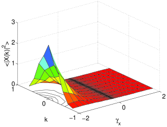
A numerical simulation of the Ginzburg-Landau equations (11) with a continuously scanned input shows that the sub-harmonic quadrature correlations appear to have a true critical point in two transverse dimensions. This result is shown in Figure (1), which graphs $\langle|X(k)|^{2}\rangle$ around $k=0$, as a function of the driving field $\gamma_{x}$ near threshold.

While these large fluctuations are occurring, we note that there are still strong non-classical correlations in the squeezed quadrature. This can be seen by analysing the relevant equations to the next order in $g_{c}$, which we also simplify by using a Gaussian factorizationStochdiagram :

$${g_{c}}\frac{\partial Y}{\partial\tau}\approx-\gamma_{y}Y+\nabla^{2}X-{g_{c}}Y\langle X^{2}\rangle-\tilde{\gamma}_{yx}X+\xi_{y}\,\,,$$ (14)

where $\tilde{\gamma}_{yx}=\gamma_{yx}+2{g_{c}}\langle XY\rangle$. In general, one can always choose an optimum local oscillator phase so that $\theta=k^{2}+\Delta_{1}+2{g_{c}}\langle XY\rangle$, in order to minimise the feedback of critical fluctuations into the squeezed quadrature at a given transverse momentum $k$. This leads to Fourier solutions which showing that entanglementDrummondFicek between the modes of momentum $k$ and $-k$ can still occur at small enough wave-vectors, resulting in a universal squeezing spectrum as a function of frequency:

$$V(\Omega)=1-\frac{1-{g_{c}}(\langle X^{2}\rangle+\gamma_{x})}{({g_{c}}\Omega/2)^{2}+\left(1+{g_{c}}(\langle X^{2}\rangle-\gamma_{x})/2\right)^{2}}\,\,.$$ (15)

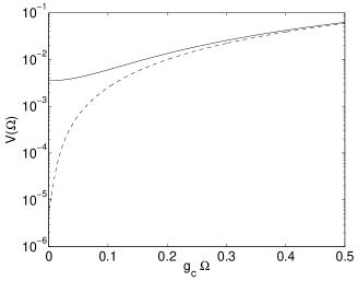
This result differs from the linearised predictions of earlier treatmentsLugiato . A graph of the resulting spectrum in the Gaussian approximation is shown in Fig (2), compared to the linearized squeezing spectrum, showing large differences near threshold.

Figure 2: Squeezing spectrum as a function of frequency, with (solid line) and without (dotted line) nonlinear corrections. The parameters used are $\gamma_{x}=0.5$, $g_{c}=0.01$.

In summary, we have shown that the planar non-equilibrium OPO with quantum noise can be mapped to a magnetic phase-transition in two dimensions. Since the present case has a scalar, real order parameter it is analogous to the uni-axial ($m=1$) magnetic order parameter case, which is known to have a thermal equilibrium Lifshitz-point phase-transition at finite temperatureHornreich79 . This demonstrates a striking resemblance between known thermal equilibrium phase-transitions, and a quantum non-equilibrium system in which quantum noise replaces thermal noise. In this system there are also quantum correlations of the emitted photons, causing quantum squeezing and entanglement. Nevertheless, this highly non-classical behavior is found only in the squeezed ($Y)$ quadrature which has no critical slowing down - and co-exists with a rather classical and universal critical fluctuation field in the conjugate ($X$) quadrature.

PDD acknowledges support from the Australian Research Council.

References

- (1) P. D. Drummond, K. J. McNeil and D. F. Walls, Optica Acta 27, 321 (1980); P. D. Drummond, K. J. McNeil and D. F. Walls, Optica Acta 28, 211 (1981).
- (2) L. A. Wu, H. J. Kimble, J. L. Hall, H. Wu, Phys. Rev. Lett. 57, 2520 (1986).
- (3) G.-L. Oppo, M. Brambilla and L. A. Lugiato, Phys. Rev. A 49, 2028 (1994); K. Staliunas, J. Mod. Opt. 42, 1261 (1995); S. Longhi and A. Geraci, Phys. Rev. A 54, 4581 (1996); M. Taki, M. San Miguel and M. Santagiustina, Phys. Rev. E 61, 2133 (2000); H. Ward, M. Taki and P. Glorieux, Opt. Lett. 27, 348 (2002).
- (4) P. D. Drummond, Phys. Rev. A 42, 6845 (1990).
- (5) A. Gatti and L. Lugiato, Phys. Rev. A 52, 1675 (1995); L. A. Lugiato, A. Gatti and E. Brambilla, J. Opt. B: Quant Semiclass. Opt 4, S176 (2002).
- (6) M. Vaupel, A. Maitre, and C. Fabre, Phys. Rev. Lett. 83, 5278 (1999) ; M. Martinelli, N. Treps, et. al., Phys. Rev. A 67, 023808 (2003).
- (7) N. Treps, N. Grosse, W. P. Bowen, C. Fabre, H. A. Bachor, and P. K. Lam, Science 301, 940 (2003).
- (8) J. P. Gollub and J. S. Langer, Rev. Mod. Phys. 71, S396 (1999).
- (9) L. I. Plimak and D.F. Walls, Phys. Rev. A 50, 2627 (1994); C. J. Mertens, T. A. B. Kennedy and S. Swain, Phys. Rev. Lett. 71, 2014 (1993); O. Veits and M. Fleischhauer, Phys. Rev. A 52, R4344 (1995); Phys. Rev. A 55, 3059 (1997).
- (10) S. Chaturvedi, K. Dechoum, and P. D. Drummond, Phys. Rev. A 65, 033805 (2002); P. D. Drummond, K. Dechoum and S. Chaturvedi, ibid., 033806 (2002).
- (11) R. M. Hornreich, M. Luban, and S. Shtrikman, Phys. Rev. Lett. 35, 1678 (1975).
- (12) A. Michelson, Phys. Rev. B 16, 577 (1977).
- (13) T. A. Kaplan, Phys. Rev. Lett. 44, 760 (1980).
- (14) R.M. Hornreich, R. Liebmann, H.G. Schuster and W. Selke, Z. Phys. B35, 91(1979); R.M. Hornreich, Journal of Magnetic Materials, 15, 387 (1980).
- (15) N. D. Mermin and H. Wagner, Phys. Rev. Lett. 17, 1133 (1966).
- (16) For a more formal stochastic procedure, see: S. Chaturvedi and P. D. Drummond, Eur. Phys. J. B 59, 251 (1999).
- (17) P. D. Drummond and Z. Ficek (eds), Quantum Squeezing (Springer-Verlag, Berlin, 2004).