Quantum-information theoretic properties of nuclei and trapped Bose gases

Abstract

Fermionic (atomic nuclei) and bosonic (correlated atoms in a trap) systems are studied from an information-theoretic point of view. Shannon and Onicescu information measures are calculated for the above systems comparing correlated and uncorrelated cases as functions of the strength of short range correlations. One-body and two-body density and momentum distributions are employed. Thus the effect of short-range correlations on the information content is evaluated. The magnitude of distinguishability of the correlated and uncorrelated densities is also discussed employing suitable measures of distance of states i.e. the well known Kullback-Leibler relative entropy and the recently proposed Jensen-Shannon divergence entropy. It is seen that the same information-theoretic properties hold for quantum many-body systems obeying different statistics (fermions and bosons).

1 Introduction

Information-theoretic methods are used in recent years for the study of quantum mechanical systems. [1]^-[17] The quantity of interest is Shannon’s information entropy for a probability distribution $p(x)$

$$S=-\int p(x)\,\ln{p(x)}\,dx$$ (1)

where $\int p(x)\,dx=1$.

An important step is the discovery of an entropic uncertainty relation (EUR),[2] which for a three-dimensional system has the form

$$S=S_{r}+S_{k}\geq 3\,(1+\ln{\pi})\simeq 6.434$$ (2)

where $S_{r}$ is the information entropy in position-space of the density distribution $\rho(\textbf{r})$ of a quantum system

$$S_{r}=-\int\rho(\textbf{r})\,\ln{\rho(\textbf{r})}\,d\textbf{r}$$ (3)

and $S_{k}$ is the information entropy in momentum-space of the corresponding momentum distribution $n(\textbf{k})$

$$S_{k}=-\int n(\textbf{k})\,\ln{n(\textbf{k})}\,d\textbf{k}$$ (4)

The density distributions $\rho(\textbf{r})$ and $n(\textbf{k})$ are normalized to one. Inequality (2), for the information entropy sum in conjugate spaces, is a joint measure of uncertainty of a quantum mechanical distribution, since a highly localized $\rho(\textbf{r})$ is associated with a diffuse $n(\textbf{k})$, leading to low $S_{r}$ and high $S_{k}$ and vice-versa. Expression (2) is an information-theoretical relation stronger than Heisenberg’s. $S$ is measured in bits if the base of the logarithm is 2 and nats (natural units of information) if the logarithm is natural.

In previous work we proposed a universal property of $S$ for the density distributions of nuclei, electrons in atoms and valence electrons in atomic clusters.[5] This property has the form

$$S=a+b\ln{N}$$ (5)

where $N$ is the number of particles of the system and the parameters $a,b$ depend on the system under consideration. It is noted that recently we have obtained the same form for systems of correlated bosons in a trap.[4] This concept was also found to be useful in a different context. Using the formalism in phase-space of Ghosh, Berkowitz and Parr,[9] we found that the larger the information entropy the better the quality of the nuclear density distribution.[10]

In previous work we employed one-body density distributions in the definition of $S$. In the present paper we introduce two-body density distributions $\rho(\textbf{r}_{1},\textbf{r}_{2})$ and the corresponding two-body momentum distributions $n(\textbf{k}_{1},\textbf{k}_{2})$. Our aim is to investigate the properties of $S$ at the two-body level for correlated densities. The correlated nucleon systems or the trapped Bose gas, in a good approximation, are studied using the lowest order approximation.[18, 19] Short-range correlations (SRC) are taken into account employing the Jastrow correlation function.[20] Thus it is of interest to examine how $S_{2}$ is affected qualitatively and quantitatively by the same form of correlations in comparison with $S_{1}$, in view of the fact that the quantities $\rho(\textbf{r}_{1},\textbf{r}_{2})$ and $n(\textbf{k}_{1},\textbf{k}_{2})$ carry more direct information for correlations than the quantities $\rho(\textbf{r})$ and $n(\textbf{k})$ which are only indirectly affected by correlations. The above procedure is repeated for an alternative measure of information i.e. Onicescu’s information energy $E$.[21] So far, only the mathematical aspects of this concept have been developed, while the physical aspects have been neglected.

A well known measure of distance of two discrete probability distributions $p_{i}^{(1)},p_{i}^{(2)}$ is the Kullback-Leibler relative entropy [22]

$$K(p_{i}^{(1)},p_{i}^{(2)})=\sum_{i}p_{i}^{(1)}\,\ln{\frac{p_{i}^{(1)}}{p_{i}^{(2)}}}$$ (6)

which for continuous probability distributions $\rho^{(1)},\rho^{(2)}$ is defined as

$$K=\int\rho^{(1)}(x)\,\ln{\frac{\rho^{(1)}(x)}{\rho^{(2)}(x)}}\,dx$$ (7)

which can be easily extended for 3-dimensional systems.

Our aim is to calculate the relative entropy (distance) between $p^{(1)}$ (correlated) and $p^{(2)}$ (uncorrelated) densities both at the one- and the two-body levels in order to assess the influence of SRC (through the correlation parameter $y$) on the distance $K$. It is noted that this is done for both systems under consideration: nuclei and trapped Bose gases. An alternative definition of distance of two probability distributions was introduced by Rao and Lin,[23, 24] i.e. a symmetrized version of $K$, the Jensen-Shannon divergence $J$ [25]

$$J(p^{(1)},p^{(2)})=H\left(\frac{p^{(1)}+p^{(2)}}{2}\right)-\frac{1}{2}H\left(p^{(1)}\right)-\frac{1}{2}H\left(p^{(2)}\right)$$ (8)

where $H(p)=-\sum_{i}p_{i}\ln{p_{i}}$ stands for Shannon’s entropy. We expect for strong SRC the amount of distinguishability of the correlated from the uncorrelated distributions is larger than the corresponding one with small SRC. We may also see the effect of SRC on the number of trials $L$ needed to distinguish $p^{(1)}$ and $p^{(2)}$ (in the sense described in [25]).

In addition to the above considerations, we connect $S_{r}$ and $S_{k}$ with fundamental quantities i.e. the root mean square radius and kinetic energy respectively. We also argue on the effect of SRC on EUR and we propose a universal relation for $S$, by extending our formalism from the one- and two-body level to the $N$-body level, which holds exactly for uncorrelated densities in trapped Bose gas, almost exactly for uncorrelated densities in nuclei (due to the additional exchange term compared to Bose gas) and it is conjectured to hold approximately for correlated densities both in nuclei and Bose gases.

The plan of the present paper is the following. In Sec. 2 we review the formulas of Kullback-Leibler relative entropy entropy $K$ and Jensen-Shannon divergence $J$, while in Sec. 3 Onicescu’s information energy $E$ is described. In Sec. 4 we present the formalism of density distributions used in present work and their applications to Shannon’s and Onicescu’s entropies. In Sec. 5 we introduce SRC in nuclei. In Sec. 6 we apply the formulas of $K$ and $J$ in correlated distributions. In Sec. 7 we present our numerical results and discussion. Finally, Sec. 8 contains our main conclusions.

2 Kullback-Leibler relative entropy and Jensen-Shannon divergence

The Kullback-Leibler relative information entropy $K$ for continuous distributions $\rho_{i}^{(1)}$ and $\rho_{i}^{(2)}$ is defined by relation (7). It measures the difference of $\rho_{i}^{(1)}$ form the reference (or apriori) distribution $\rho_{i}^{(2)}$. It satisfies: $K\geq 0$ for any distributions $\rho_{i}^{(1)}$ and $\rho_{i}^{(2)}$. It is a measure which quantifies the distinguishability (or distance) of $\rho_{i}^{(1)}$ from $\rho_{i}^{(2)}$, employing a well-known concept in standard information theory. In other words it describes how close $\rho_{i}^{(1)}$ is to $\rho_{i}^{(2)}$ by carrying out observations or coin tossing, namely $L$ trials (in the sense described in [25]). We expect for strong SRC the amount of distinguishability of the correlated $\rho_{i}^{(1)}$ and the uncorrelated distributions $\rho_{i}^{(2)}$ is larger than the corresponding one with small SRC.

However, the distance $K$ does not satisfy the triangle inequality and in addition is i) not symmetric ii) unbounded and iii) not always well defined.[25] To avoid these difficulties Rao and Lin [23, 24] introduced a symmetrized version of $K$ (recently discused in [25]), the Jensen-Shannon divergence $J$ defined by relation (8). $J$ is minimum for $\rho^{(1)}=\rho^{(2)}$ and maximum when $\rho^{(1)}$ and $\rho^{(2)}$ are two distinct distributions, when $J=\ln{2}$. In our case $J$ can be easily generalized for continuous density distributions. For $J$ minimum the two states represented by $\rho^{(1)}$ and $\rho^{(2)}$ are completely indistinguishable, while for $J$ maximum they are completely distinguishable. It is expected that for strong SRC the amount of distinguishability can be further examined by using Wooter’s criterion.[25] Two probability distributions $\rho^{(1)}$ and $\rho^{(2)}$ are distinguishable after $L$ trials $(L\rightarrow\infty)$ if and only if $\left(J(\rho^{(1)},\rho^{(2)})\right)^{\frac{1}{2}}>\frac{1}{\sqrt{2L}}$.

The present work is a first step to examine the problem of comparison of probability distributions (for nuclei and bosonic systems) which is an area well developed in statistics, known as information geometry.[23]

3 Onicescu’s information energy

Onicescu tried to define a finer measure of dispersion distributions than that of Shannon’s information entropy.[21] Thus, he introduced the concept of information energy $E$. For a discrete probability distribution $(p_{1},p_{2},\ldots,p_{k})$ the information energy $E$ is defined by

$$E=\sum_{i}^{k}p_{i}^{2}$$ (9)

which is extended for a continuous density distribution $\rho(x)$ as

$$E=\int\rho^{2}(x)\,dx$$ (10)

The meaning of (10) can be seen by the following simple argument: For a Gaussian distribution of mean value $\mu$, standard deviation $\sigma$ and normalized density

$$\rho(x)=\frac{1}{\sqrt{2\pi}\sigma}\,\textrm{exp}\left[-\frac{(x-\mu)^{2}}{2\sigma^{2}}\right]$$ (11)

relation (10) gives

$$E=\frac{1}{2\pi\sigma^{2}}\int_{-\infty}^{\infty}\textrm{exp}\left[-\frac{(x-\mu)^{2}}{\sigma^{2}}\right]\,dx=\frac{1}{2\sigma\sqrt{\pi}}$$ (12)

$E$ is maximum if one of the $p_{i}$’s equals 1 and all the others are equal to zero i.e. $E_{max}=1$, while $E$ is minimum when $p_{1}=p_{2}=\ldots=p_{k}=\frac{1}{k}$, hence $E_{min}=\frac{1}{k}$ (total disorder). The fact that $E$ becomes minimum for equal probabilities (total disorder), by analogy with thermodynamics, it has been called information energy, although it does not have the dimension of energy.[26]

It is seen from (12) that the greater the information energy, the more concentrated is the probability distribution, while the information content decreases. $E$ and information content are reciprocal, hence one can define the quantity

$$O=\frac{1}{E}$$ (13)

as a measure of the information content of a quantum system corresponding to Onicescu’s information energy.

Relation (10) is extended for a 3-dimensional spherically symmetric density distribution $\rho(\textbf{r})$

$$E_{r}=\int\rho^{2}(\textbf{r})\,d\textbf{r}$$

$$E_{k}=\int n^{2}(\textbf{k})\,d\textbf{k}$$ (14)

in position and momentum space respectively, where $n(\textbf{k})$ is the corresponding density distribution in momentum space.

$E_{r}$ has dimension of inverse volume, while $E_{k}$ of volume. Thus the product $E_{r}E_{k}$ is dimensionless and can serve as a measure of concentration (or information content) of a quantum system. It is also seen from (12),(13) that $E$ increases as $\sigma$ decreases (or concentration increases) and the information (or uncertainty) decreases. Thus $O$ and $E$ are reciprocal. In order to be able to compare $O$ with Shannon’s entropy $S$, we redifine $O$ as

$$O=\frac{1}{E_{r}E_{k}}$$ (15)

as a measure of the information content of a quantum system in both position and momentum spaces, inspired by Onicescu’s definition.

4 Density Matrices and Information entropies

Let $\Psi({\bf r}_{1},{\bf r}_{2},\cdots,{\bf r}_{A})$ be the wave function that describes the nuclei or the trapped Bose gases and depends on 3A coordinates as well as on spin and isospin (in nuclei). The one-body density matrix is defined in [27]

$$\rho({\bf r}_{1},{\bf r}_{1}^{\prime})=\int\Psi^{*}({\bf r}_{1},{\bf r}_{2},\cdots,{\bf r}_{A})\Psi({\bf r}_{1}^{\prime},{\bf r}_{2},\cdots,{\bf r}_{A})d{\bf r}_{2}\cdots d{\bf r}_{A}$$ (16)

while the two-body density matrix by

$$\rho({\bf r}_{1},{\bf r}_{2};{\bf r}_{1}^{\prime},{\bf r}_{2}^{\prime})=\int\Psi^{*}({\bf r}_{1},{\bf r}_{2},\cdots,{\bf r}_{A})\Psi({\bf r}_{1}^{\prime},{\bf r}_{2}^{\prime},\cdots,{\bf r}_{A})d{\bf r}_{3}\cdots d{\bf r}_{A}$$ (17)

The above density matrices are related by

$$\rho({\bf r}_{1},{\bf r}_{1}^{\prime})=\frac{1}{A-1}\int\rho({\bf r}_{1},{\bf r}_{2};{\bf r}_{1}^{\prime},{\bf r}_{2})d{\bf r}_{2}$$ (18)

where the integration is carried out over the radius vectors ${\bf r}_{2},\cdots,{\bf r}_{A}$ and summation over spin (or isospin) variables is implied. The corresponding definitions in momentum space are similar. The two-body density distribution $\rho({\bf r}_{1},{\bf r}_{2})$ which is a key quantity in the present work, is defined as the diagonal part of the two-body density matrix

$$\rho({\bf r}_{1},{\bf r}_{2})=\rho({\bf r}_{1},{\bf r}_{2};{\bf r}_{1}^{\prime},{\bf r}_{2}^{\prime})\mid_{{\bf r}_{1}^{\prime}={\bf r}_{1},{\bf r}_{2}^{\prime}={\bf r}_{2}}$$ (19)

and expresses the joint probability of finding two nucleons or two atoms at the positions ${\bf r}_{1}$ and ${\bf r}_{2}$, respectively. The density distribution is given by the diagonal part of the one-body density matrix, that is

$$\rho({\bf r}_{1})=\rho({\bf r}_{1},{\bf r}_{1}^{\prime})|_{{\bf r}_{1}={\bf r}_{1}^{\prime}}$$ (20)

or by the equivalent integral

$$\rho({\bf r}_{1})=\frac{1}{A-1}\int\rho({\bf r}_{1},{\bf r}_{2})d{\bf r}_{2}$$ (21)

The two-body momentum distribution $n({\bf k}_{1},{\bf k}_{2})$ is given by a particular Fourier transform of the $\rho({\bf r}_{1},{\bf r}_{2};{\bf r}_{1}^{\prime},{\bf r}_{2}^{\prime})$, that is

$$n({\bf k}_{1},{\bf k}_{2})=\frac{1}{(2\pi)^{6}}\int\rho({\bf r}_{1},{\bf r}_{2};{\bf r}_{1}^{\prime},{\bf r}_{2}^{\prime})\exp[i{\bf k}_{1}({\bf r}_{1}-{\bf r}_{1}^{\prime})]\exp[i{\bf k}_{2}({\bf r}_{2}-{\bf r}_{2}^{\prime})]d{\bf r}_{1}d{\bf r}_{1}^{\prime}d{\bf r}_{2}d{\bf r}_{2}^{\prime}$$ (22)

In the independent particle model, where the nucleons are considered to move independently in nuclei, the $\Psi({\bf r}_{1},{\bf r}_{2},\cdots,{\bf r}_{A})$ is a Slater determinant. In this case it is easy to show that the two-body density matrix is given by the relation

$$\rho_{SD}({\bf r}_{1},{\bf r}_{2};{\bf r}_{1}^{\prime},{\bf r}_{2}^{\prime}) = \sum_{i,j}\phi_{i}({\bf r}_{1})\phi_{i}({\bf r}_{1}^{\prime})\phi_{j}({\bf r}_{2})\phi_{j}({\bf r}_{2}^{\prime})-\sum_{i,j}\phi_{i}({\bf r}_{1})\phi_{j}({\bf r}_{1}^{\prime})\phi_{j}({\bf r}_{2})\phi_{i}({\bf r}_{2}^{\prime})$$ (23)

$$= \rho_{SD}({\bf r}_{1},{\bf r}_{1}^{\prime})\rho_{SD}({\bf r}_{2},{\bf r}_{2}^{\prime})-\rho_{SD}({\bf r}_{1},{\bf r}_{2}^{\prime})\rho_{SD}({\bf r}_{2},{\bf r}_{1}^{\prime})$$

where $\phi_{i}({\bf r})$ is the single-particle wave function normalized to one and

$$\rho_{SD}({\bf r}_{1},{\bf r}_{1}^{\prime})=\sum_{i}\phi_{i}({\bf r}_{1})\phi_{i}({\bf r}_{1}^{\prime})$$

In Bose gases the many-body ground-state wave function $\Psi({\bf r}_{1},{\bf r}_{2},\cdots,{\bf r}_{A})$ is a product of $A$ identical single-particle ground-state wave functions i.e.

$$\Psi({\bf r}_{1},{\bf r}_{2},\cdots,{\bf r}_{A})=\phi_{0}({\bf r}_{1})\phi_{0}({\bf r}_{2})\cdots\phi_{0}({\bf r}_{A})$$ (24)

where $\phi_{0}({\bf r}_{1})$ is the normalized to one ground-state single-particle wave function describing bosonic atoms. The two-body density matrix in a Bose gas, is given by the relation

$$\rho_{0}({\bf r}_{1},{\bf r}_{2};{\bf r}_{1}^{\prime},{\bf r}_{2}^{\prime})=\rho_{0}({\bf r}_{1},{\bf r}_{1}^{\prime})\rho_{0}({\bf r}_{2},{\bf r}_{2}^{\prime})$$ (25)

where

$$\rho_{0}({\bf r}_{1},{\bf r}_{1}^{\prime})=\phi_{0}({\bf r}_{1})\phi_{0}({\bf r}_{1}^{\prime})$$ (26)

We consider that the atoms of the Bose gases are confined in an isotropic HO well, where $\phi_{0}({\bf r})=(1/(\pi b^{2}))^{3/4}\exp[-r^{2}/(2b^{2})]$.

As the mean field approach fails to incorporate the interparticle correlation which is necessary for the description of the correlated nuclei or trapped Bose gases, we introduce the repulsive interactions through the Jastrow correlation function $f({\bf r}_{1}-{\bf r}_{2})$ [20]. The correlated nucleon systems or the Bose gases, in a good approximation, can be studied using the lowest order approximation,[18, 19] where the correlated two-body density matrices in nuclei and Bose gases have the following forms respectively

$$\rho({\bf r}_{1},{\bf r}_{2};{\bf r}_{1}^{\prime},{\bf r}_{2}^{\prime})=N\rho_{SD}({\bf r}_{1},{\bf r}_{2};{\bf r}_{1}^{\prime},{\bf r}_{2}^{\prime})f({\bf r}_{1}-{\bf r}_{2})f({\bf r}_{1}^{\prime}-{\bf r}_{2}^{\prime})$$ (27)

$$\rho({\bf r}_{1},{\bf r}_{2};{\bf r}_{1}^{\prime},{\bf r}_{2}^{\prime})=N\rho_{0}({\bf r}_{1},{\bf r}_{2};{\bf r}_{1}^{\prime},{\bf r}_{2}^{\prime})f({\bf r}_{1}-{\bf r}_{2})f({\bf r}_{1}^{\prime}-{\bf r}_{2}^{\prime})$$ (28)

In the present work, in the case of nuclei and trapped Bose gas, the normalization factor $N$, is calculated by the normalization condition

$$\int\rho(\textbf{r}_{1},\textbf{r}_{2})\,d\textbf{r}_{1}\,d\textbf{r}_{2}=1$$ (29)

The same holds for $n(\textbf{k}_{1},\textbf{k}_{2})$

$$\int n(\textbf{k}_{1},\textbf{k}_{2})\,d\textbf{k}_{1}\,d\textbf{k}_{2}=1$$ (30)

The Jastrow correlation function $f(\textbf{r}_{1}-\textbf{r}_{2})$ both in the case of nuclei and trapped Bose gas is taken to be of the form

$$f(\textbf{r}_{1}-\textbf{r}_{2})=1-\textrm{exp}[-y\,\frac{(\textbf{r}_{1}-\textbf{r}_{2})^{2}}{b^{2}}]$$ (31)

The uncorrelated case corresponds to $y\rightarrow\infty$, while SRC increase as $y$ decreases. The above ansatz has the advantage that it leads to analytical forms for the $\rho(\textbf{r}_{1},\textbf{r}_{2})$, $n(\textbf{k}_{1},\textbf{k}_{2})$, $\rho(\textbf{r})$ and $n(\textbf{k})$.

The one-body Shannon information entropy both in position- and momentum- space are defined in (3) and (4), where the total sum is

$$S_{1}=S_{1r}+S_{1k}$$ (32)

The two-body Shannon information entropy both in position- and momentum- space and in total are defined respectively [28, 29]

$$S_{2r}=-\int\rho({\bf r}_{1},{\bf r}_{2})\ln\rho({\bf r}_{1},{\bf r}_{2})d{\bf r}_{1}d{\bf r}_{2}$$ (33)

$$S_{2k}=-\int n({\bf k}_{1},{\bf k}_{2})\ln n({\bf k}_{1},{\bf k}_{2})d{\bf k}_{1}d{\bf k}_{2}$$ (34)

$$S_{2}=S_{2r}+S_{2k}$$ (35)

The one-body Onicescu information entropy is already defined in (3) and (15), where the generalization to the two-body information entropy is straightforward and is given by

$$O_{2}=\frac{1}{E_{2r}E_{2k}}$$ (36)

where

$$E_{2r} = \int\rho^{2}({\bf r}_{1},{\bf r}_{2})d{\bf r}_{1}d{\bf r}_{2}$$

$$E_{2k} = \int n^{2}({\bf k}_{1},{\bf k}_{2})d{\bf k}_{1}d{\bf k}_{2}$$ (37)

It is easy to prove that in the case of the uncorrelated trapped Bose gas

$$S_{2}=2S_{1}$$ (38)

and

$$O_{2}=O_{1}^{2}$$ (39)

It is worth noting that the above relations hold only approximately in finite nuclei (see Table 1), due to the additional exchange term, originating from the antisymmetry of the nuclear wave function. There is an exception in the case of ⁴He, where it holds exactly due to the absence of the exchange term.

5 Introduction of SRC in nuclei

We consider that the single particle wave functions, which describe the nucleons is harmonic oscillator type. In order to incorporate the nucleon-nucleon (or atom-atom) correlations, as we mention in the previous section, we apply the lowest order approximation. In this case the two-body density distribution, for ⁴He, takes the following form

$$\rho^{{}^{4}He}({\bf r}_{1},{\bf r}_{2})=\rho^{{}^{4}He}_{SD}({\bf r}_{1},{\bf r}_{2})+\rho^{{}^{4}He}_{cor}({\bf r}_{1},{\bf r}_{2})$$ (40)

The first term of the right-hand side of Eq. (40) which represents the uncorrelated part of the two-body sensity distribution, has the form

$$\rho^{{}^{4}He}_{SD}({\bf r}_{1},{\bf r}_{2})=\frac{1}{\pi^{3}b^{6}}\exp[-r_{1b}^{2}]\exp[-r_{2b}^{2}]$$ (41)

and the second term which represents the correlated part of the two-body density distribution, is written

$$\rho^{{}^{4}He}_{cor}({\bf r}_{1},{\bf r}_{2}) = \frac{1}{\pi^{3}b^{6}}\exp[-r_{1b}^{2}]\exp[-r_{2b}^{2}]$$ (42)

$$\times\left(N\left(1-\exp[-y({\bf r}_{1b}-{\bf r}_{2b})^{2}]\right)^{2}-1\right)$$

where $\textbf{r}_{b}={\bf r}/b$.

In the above expression $b$ is the width of the HO potential and $N$ is the normalization constant which ensures that $\int\rho^{{}^{4}He}_{cor}({\bf r}_{1},{\bf r}_{2})d{\bf r}_{1}d{\bf r}_{2}=1$ and has the form

$$N=\left(1-\frac{2}{(1+2y)^{3/2}}+\frac{1}{(1+4y)^{3/2}}\right)^{-1}$$ (43)

The density distribution can be written also in the form

$$\rho^{{}^{4}He}(r)=\rho_{SD}^{{}^{4}He}(r)+\rho_{cor}^{{}^{4}He}(r)$$ (44)

The two-body momentum distribution is given also by the formula

$$n^{{}^{4}He}({\bf k}_{1},{\bf k}_{2})=n^{{}^{4}He}_{SD}({\bf k}_{1},{\bf k}_{2})+n^{{}^{4}He}_{cor}({\bf k}_{1},{\bf k}_{2})$$ (45)

where, as in the case of two-body density distribution, the uncorrelated part has the form

$$n^{{}^{4}He}_{SD}({\bf k}_{1},{\bf k}_{2})=\frac{b^{6}}{\pi^{3}}\exp[-k_{1b}^{2}]\exp[-k_{2b}^{2}]$$ (46)

and the correlated part is written as

$$n^{{}^{4}He}_{cor}({\bf k}_{1},{\bf k}_{2}) = \frac{b^{6}}{\pi^{3}}\exp[-k_{1b}^{2}]\exp[-k_{2b}^{2}]$$

$$\times\left(N(1-\frac{1}{(1+4y)^{3/2}}\exp[-\frac{y}{1+4y}({\bf k}_{1b}-{\bf k}_{2b})^{2}])^{2}-1\right)$$

where $\textbf{k}_{b}=\textbf{k}\,b$.
The momentum distribution is given also by the relation

$$n^{{}^{4}He}(k)=n_{SD}^{{}^{4}He}(k)+n_{cor}^{{}^{4}He}(k)$$ (48)

In the present work, we extend our calculations in nuclei heavier than ${}^{4}\textrm{He}$ (¹²C, ¹⁶O and ⁴⁰Ca) based on the fact that the high-momentum tails of $n(k)$ are almost the same for all nuclei with $A\geq 4$.[11, 30] Inspired by previous work [31, 32] we suggest a practical method to calculate the one- and two-body density and momentum distributions for nuclei heavier than ⁴He. The theoretical scheme of the method combines the mean-field predictions of the two-body density distributions and two-body momentum distributions of various nuclei with their correlated part of ⁴He. Specifically, in our treatment we consider the following forms

$$\rho^{A}({\bf r}_{1},{\bf r}_{2})=\rho^{A}_{SD}({\bf r}_{1},{\bf r}_{2})+\rho^{{}^{4}\textrm{He}}_{cor}({\bf r}_{1},{\bf r}_{2})$$ (49)

$$n^{A}({\bf k}_{1},{\bf k}_{2})=n^{A}_{SD}({\bf k}_{1},{\bf k}_{2})+n^{{}^{4}\textrm{He}}_{cor}({\bf k}_{1},{\bf k}_{2})$$ (50)

From the above expressions it is obvious that the uncorrelated part of the $\rho(\textbf{r}_{1},\textbf{r}_{2})$ and $n(\textbf{k}_{1},\textbf{k}_{2})$ originate from the independent particle model for every nucleus separately, where the correlated part in each nucleus is that coming from the nucleus ⁴He. The $\rho(\textbf{r})$ and $n(\textbf{k})$ have a similar form.

It should be emphasized that in the uncorrelated case the additional information which is contained in $\rho(\textbf{r}_{1},\textbf{r}_{2})$ and $n(\textbf{k}_{1},\textbf{k}_{2})$ in nuclei, compared to the trapped Bose gas is the statistical correlations which come from the antisymmetry character of the many-body wave function of nuclei. Moreover, in the correlated case the $\rho(\textbf{r}_{1},\textbf{r}_{2})$ and $n(\textbf{k}_{1},\textbf{k}_{2})$ contain additional information which originate from the character of the nuleon-nucleon interaction, making our model more realistic and the description more complete. It is of interest to study how the correlations (both statistical and dynamical) affect quantitatively and qualitatively the various kinds of information entropy.

6 Application of the Formalism of Relative Entropy and Jensen-Shannon divergence for Correlated Densities

The relative entropy is a measure of distinguishability or distance of two states. It is defined, generalizing (7), by

$$K=\int\psi^{2}(\textbf{r})\ln{\frac{\psi^{2}(\textbf{r})}{\phi^{2}(\textbf{r})}}\,d\textbf{r}$$ (51)

In our case $\psi(\textbf{r})$ is the correlated case and $\phi(\textbf{r})$ the uncorrelated one. Thus

$$K_{1r}=\int\rho(\textbf{r})\,\ln{\frac{\rho(\textbf{r})}{\rho^{\prime}(\textbf{r})}}\,d\textbf{r}$$ (52)

where $\rho(\textbf{r})$ is the correlated one-body density and $\rho^{\prime}(\textbf{r})$ is the uncorrelated one-body density.

A corresponding formula holds in momentum-space

$$K_{1k}=\int n(\textbf{k})\,\ln{\frac{n(\textbf{k})}{n^{\prime}(\textbf{k})}}\,d\textbf{k}$$ (53)

where $n(\textbf{k})$ is the correlated one-body density and $n^{\prime}(\textbf{k})$ is the uncorrelated one.

For the two-body case we have

$$K_{2r}=\int\rho(\textbf{r}_{1},\textbf{r}_{2})\,\ln{\frac{\rho(\textbf{r}_{1},\textbf{r}_{2})}{\rho^{\prime}(\textbf{r}_{1},\textbf{r}_{2})}}\,d\textbf{r}_{1}d\textbf{r}_{2}$$ (54)

where $\rho(\textbf{r}_{1},\textbf{r}_{2})$ is the correlated two-body density in position-space and $\rho^{\prime}(\textbf{r}_{1},\textbf{r}_{2})$ is the uncorrelated one.

The generalization to momentum- space is straightforward

$$K_{2k}=\int n(\textbf{k}_{1},\textbf{k}_{2})\ln{\frac{n(\textbf{k}_{1},\textbf{k}_{2})}{n^{\prime}(\textbf{k}_{1},\textbf{k}_{2})}}\,d\textbf{k}_{1}d\textbf{k}_{2}$$ (55)

where $n(\textbf{k}_{1},\textbf{k}_{2})$ is the correlated two-body density in momentum-space and $n^{\prime}(\textbf{k}_{1},\textbf{k}_{2})$ is the uncorrelated one.

For the Jensen-Shannon divergence $J$ we may write formulas for $J_{1}$ (one-body) and $J_{2}$ (two-body), employing definition (8) and putting the corresponding correlated $\rho^{(1)}$ and uncorrelated $\rho^{(2)}$ distributions in position- and momentum- spaces. We calculate $K$ and $J$ in position- and momentum- spaces, for nuclei and bosons.

7 Numerical results and discussion

For the sake of symmetry and simplicity we put the width of the HO potential $b=1$. Actually for $b=1$ in the case of uncorrelated case it is easy to see that $S_{1r}=S_{1k}$ and also $S_{2r}=S_{2k}$ (the same holds for Onicescu entropy), while when $b\neq 1$ there is a shift of the values of $S_{1r}$ and $S_{1k}$ by an additive factor $\ln{b^{3}}$. However, the value of $b$ does not affect directly the total information entropy $S$ (and also $O$). $S$ and $O$ are just functions of the correlation parameter $y$.

Nucleus	$S_{1}$	$S_{2}$	$O_{1}$	$\sqrt{O_{2}}$
4He	6.43418	12.86836	248.05	248.05
12C	7.50858	15.00784	922.60	921.15
16O	7.60692	15.20890	1057.25	1055.77
40Ca	8.43472	16.88498	2685.72	2711.75

Table 1: The values of the Shannon and Onicescu information entropy (both one and two body) for various nuclei $s$-$p$ and $s$-$d$ shell nuclei.

In Fig. 1 we present the Shannon information entropy $S_{1}$ using relation (32) and $S_{2}$ using relation (35) in nuclei $(^{12}\textrm{C})$ and trapped Bose gas as functions of the correlation parameter $\ln{(\frac{1}{y})}$. It is seen that $S_{1}$ and $S_{2}$ increase almost linearly with the strength of SRC i.e. $\ln{(\frac{1}{y})}$ in both systems. The relations $S_{2}=2S_{1}$ and $O_{2}=O_{1}^{2}$ hold exactly for the uncorrelated densities in trapped Bose gas, while the above relations are almost exact for the uncorrelated densities in nuclei and in the case of correlated densities both in nuclei and trapped Bose gas. A similar behavior is seen for all nuclei considered in the present work (⁴He, ¹⁶O, ⁴⁰Ca).

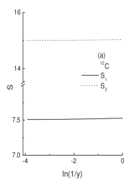
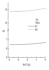
Figure 1: The Shannon information entropy one-body $S_{1}$ and two-body $S_{2}$ (a) in nuclei ¹²C and (b) in a trapped Bose gas (TBG).

Values of $S_{1}$, $S_{2}$, $O_{1}$, $O_{2}$ for various nuclei in the uncorrelated case, are shown in Table 1. The relations (38) and (39) are satisfied exactly only in the case of ⁴He. However, for the other nuclei, due to the additional exchange term in the nuclear wave function, the relations (38) and (39) hold only approximately (the differences are of order $0.03\%-0.09\%$ for $S$ and $0.14\%-0.96\%$ for $O$).

In Fig. 2 we present the decomposition of $S$ in coordinate and momentum spaces, for the sake of comparison i.e. $S_{1r}$, $S_{1k}$, $S_{2r}$, $S_{2k}$ for ${}^{16}\textrm{O}$ and trapped Bose gas employing (3), (4), (33), (34). The most striking feature concluded from the above Figures is the similar behavior between $S_{1r}$ and $S_{2r}$ and also $S_{1k}$ and $S_{2k}$ respectively.

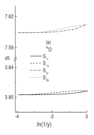
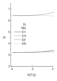
Figure 2: The Shannon information entropy (one- and two-body) both in coordinate- and momentum-space (a) in nuclei ¹⁶O and (b) in a trapped Bose gas (TBG).

In Fig. 3 we plot the Onicescu information entropy both one-body $(O_{1})$ and two-body $(O_{2})$ for nuclei $(^{12}\textrm{C},^{40}\textrm{Ca})$ and trapped Bose gas (relations (15), (36)). We conclude by noting once again the strong similarities of the behavior between one- and two-body Onicescu entropy.

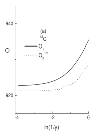
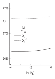
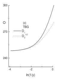
Figure 3: The Onicescu information entropy (both one- and two-body) (a) in ¹²C, (b) in ⁴⁰Ca and (c) in a trapped Bose gas (TBG).

It is interesting to observe the correlation of the rms radii $\sqrt{\langle r^{2}\rangle}$ with $S_{r}$ as well as the corresponding behavior of the mean kinetic energy $\langle T\rangle$ with $S_{k}$, as functions of the strength of SRC $\ln{(\frac{1}{y})}$ for the ${}^{16}\textrm{O}$ nucleus and trapped Bose gas. This is done in Fig. 4 for $\sqrt{\langle r^{2}\rangle}$ and Fig. 5 for $\langle T\rangle$ after apllying the suitable rescaling. The corresponding curves are similar for nuclei and trapped Bose gas.

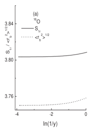
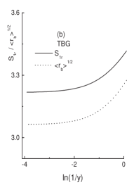
Figure 4: The mean-square radius and the Shannon information entropy $S_{1r}$ as a function of the correlation parameter $\ln{(\frac{1}{y})}$, (a) in nuclei ¹⁶O and (b) in a trapped Bose gas (TBG).

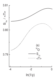
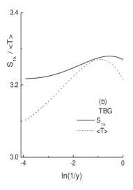
Figure 5: The mean kinetic energy $\langle T\rangle$ (in $\hbar\omega$ units) and the Shannon information entropy $S_{1k}$ as a function of the correlation parameter $\ln{(\frac{1}{y})}$, (a) in nuclei ¹⁶O and (b) in a trapped Bose gas (TBG).

A well-known concept in information theory is the distance between the probability distributions $\rho_{i}^{(1)}$ and $\rho^{(2)}$, in our case the correlated and the uncorrelated distributions respectively. A measure of distance is the Kullback-Leibler relative entropy $K$ defined previously. The correlated and uncorrelated cases are compared for the one-body case $(K_{1})$ in Fig. 6 and the the two-body case $(K_{2})$ in Fig. 7 for nuclei $(^{4}\textrm{He},^{16}\textrm{O},^{40}\textrm{Ca})$ and trapped Bose gas, decomposing in position- and momentum-spaces according to (52)-(55). It is seen that $K_{1r}$, $K_{2r}$ increase as the strength of SRC increases, while $K_{1k}$, $K_{2k}$ have a maximum at a certain value of $\ln{(\frac{1}{y})}$ depending on the system under consideration.

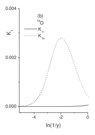
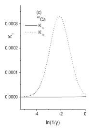
Figure 6: The one- body Kullback-Leibler relative entropy both in coordinate- and momentum-space, in nuclei (a) ⁴He, (b) ¹⁶O and (c) ⁴⁰Ca.

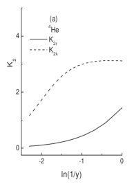
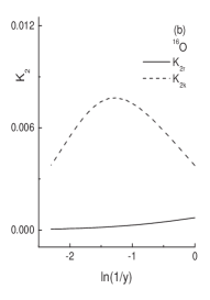
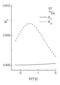
Figure 7: The two-body Kullback-Leibler relative entropy both in coordinate- and momentum-space, in nuclei (a) ⁴He, (b) ¹⁶O and c) ⁴⁰Ca.

Calculations are also carried out for the Jensen-Shannon divergence for one-body density distribution ($J_{1}$ entropy) as function of $\ln{(\frac{1}{y})}$ for nuclei and trapped Bose gas, decomposed in position- and momentum- spaces (Fig. 8). We observe again that $J_{1}$ increases with the strength of SRC in position-space, while in most cases in momentum-space there is a maximum for a certain value of $\ln{(\frac{1}{y})}$. It is verified that $0<J<\ln{2}$ as expected theoretically.[25]

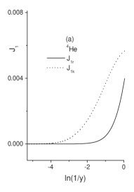
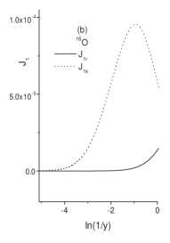
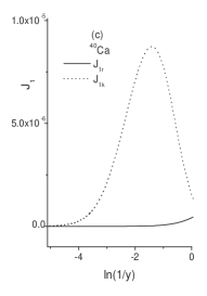
Figure 8: The one-body Jensen-Shannon divergence entropy both in coordinate- and momentum-space, in nuclei (a) ⁴He, (b) ¹⁶O and (c) ⁴⁰Ca.

It is noted that the dependence of the various kinds of information entropy on the correlation parameter $\ln{(\frac{1}{y})}$ is studied up to the value $\ln{(\frac{1}{y})}=0$ $(y=1)$, which is already unrealistic corresponding to strong SRC. In addition, lowest order approximation does not work well beyond that value. In this case three-body terms should be included but this prospect is out of the scope of the present work.

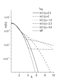
Figure 9: The momentum distribution $n(k)$ of ⁴He for various values of the correlation parameter $\ln{(\frac{1}{y})}$. The case MF (mean field) corresponds to the uncorrelated case $(y\rightarrow\infty).$

For very strong SRC the momentum distribution $n(k)$ exhibits a similar behavior with the mean field $(y\rightarrow\infty)$. This is illustrated in Fig. 9, where we present $n(k)$ for various values of $\ln{(\frac{1}{y})}$. It is seen that for small and large SRC the tail of $n(k)$ disappears. That is why for small and large SRC the relative entropy ($K_{1k}$ and $J_{1k}$) is small, while in between shows a maximum (Fig. 6, 8). A similar trend of $n(\textbf{k}_{1},\textbf{k}_{2})$ for large SRC explains also the maximum of the relative entropy $K_{2k}$ in Fig. 7.

8 Conclusions and final comment

Our main conclusions are the following

• Increasing the SRC (i.e. the parameter $\ln{(\frac{1}{y})}$) the information entropies $S$, $O$, $K$ and $J$ increase. A comparison leads to the conclusion that the correlated systems have larger values of entropies than the uncorrelated ones.

• There is a similar behavior of the entropies as functions of correlations for both systems (nuclei and trapped Bose gas) although they obey different statistics (fermions and bosons).

• There is a correlation of $\sqrt{\langle r^{2}\rangle}$ with $S_{r}$ and $\langle T\rangle$ with $S_{k}$ in the sense that they have the same behavior as a function of the correlation parameter $\ln{(\frac{1}{y})}$. These results can lead us to relate the theoretical quantities $S_{r}$ and $S_{k}$ with experimental ones like charge form factor, charge density distribution, and momentum distribution, radii, etc. A recent paper addressed in that problem.[33]

• The relations $S_{2}=2S_{1}$ and $O_{2}=O_{1}^{2}$ hold exactly for the uncorrelated densities in trapped Bose gas while the above relations are almost exact for the uncorrelated densities and in the case of correlated densities both in nuclei and trapped Bose gas. In previous work we proposed the universal relation $S_{1}=S_{r}+S_{k}=a+b\,\ln{N}$ where $N$ is the number of particles of the system either fermionic (nucleus, atom, atomic cluster) or bosonic (correlated atoms in a trap). Thus in our case

  $$S_{2}=2(a+b\,\ln{N})$$

  For 3-body distributions $\rho(\textbf{r}_{1},\textbf{r}_{2},\textbf{r}_{3})$ and $n(\textbf{k}_{1},\textbf{k}_{2},\textbf{k}_{3})$

  $$S_{3}=3\,(a+b\,\ln{N})$$

  and generalizing for the $N$-body distributions $\rho(\textbf{r}_{1},\textbf{r}_{2},\ldots,\textbf{r}_{N})$ and $n(\textbf{k}_{1},\textbf{k}_{2},\ldots,\textbf{k}_{N})$

  $$S_{N}=N\,(a+b\,\ln{N})$$

  This is exact for the uncorrelated trapped Bose gas, almost exact in correlated nuclei $(N=1,2)$ and it is conjectured that it holds approximately for correlated systems (which has still to be proved for $N\geq 3$).

• The entropic uncertainty relation (EUR) is

  $$S=S_{r}+S_{k}\geq 6.434$$

  It is well-known that the lower bound is attained for a Gaussian distribution (i.e. the case of ${}^{4}\textrm{He}$ uncorrelated). In all cases studied in the present work EUR is verified.

  A final comment seems appropriate. In general, the calculation of $\rho({\bf r}_{1},{\bf r}_{2})$ and $n({\bf k}_{1},{\bf k}_{2})$ is a problem very hard to be solved, especially in the case of nuclei, in the framework of short range correlations. Just a few works are addressed in that problem.[34, 35, 36] In the present work we tried to treat the problem in an approximate but self-consistent way in the sense that the calculations of $\rho({\bf r}_{1},{\bf r}_{2})$ and $n({\bf k}_{1},{\bf k}_{2})$ are based in the same $\rho({\bf r}_{1},{\bf r}_{2};{\bf r}_{1}^{\prime},{\bf r}_{2}^{\prime})$, which is the generating function of the above quantities. As a consequence the information entropy $S_{2}=S_{2r}+S_{2k}$ is derived also in a self-consistent way and there is a direct link between $S_{2r}$ and $S_{2k}$, as well as the other kinds of information entropies which are studied in the present work.

References

- [1] M. Ohya, and D. Petz, Quantum Entropy and Its Use ( Springer-Verlag, Berlin; New York, 1993).
- [2] I. Bialynicki-Birula, and J. Mycielski, Commun. Math. Phys 44 (1975) 129.
- [3] C. P. Panos, and S. E. Massen, Int. J. Mod. Phys. E6 (1997) 497 .
- [4] S. E. Massen, Ch. C. Moustakidis, and C. P. Panos, Phys. Let. A64 (2002) 131.
- [5] S. E. Massen, and C. P. Panos, Phys. Lett. A246 (1998) 530.
- [6] S. E. Massen, and C. P. Panos, Phys. Lett. A280 (2001) 65.
- [7] S. R. Gadre, S. B. Sears, S. J. Chakravorty, and R. D. Bendale, Phys. Rev. A32 (1985) 2602.
- [8] S. R. Gadre, and R. D. Bendale, Phys. Rev. A36 (1987) 1932.
- [9] S. K. Ghosh, M. Berkowitz, and R. G. Parr, Proc. Natl. Acad. Sc. USA 81 (1984) 8028.
- [10] G. A. Lalazissis, S. E. Massen, C. P. Panos, and S. S. Dimitrova, Int. J. Mod. Phys. E7 (1998) 485.
- [11] Ch. C. Moustakidis, S. E. Massen, C. P. Panos, M. E. Grypeos, and A. N. Antonov, Phys. Rev. 64 (2001) 014314.
- [12] C. P. Panos, S. E. Massen, and C. G. Koutroulos, Phys. Rev. 63 (2001) 064307.
- [13] C. P. Panos, Phys. Lett. A289 (2001) 287.
- [14] S. E. Massen, Phys. Rev. C67 (2003) 014314.
- [15] Ch.C. Moustakidis, and S.E. Massen, Phys. Rev. B71 (2003) 045102.
- [16] S. E. Massen, Ch. C. Moustakidis, and C. P. Panos, Focus on Boson Research (Nova Publishers, editor A. V. Ling) In press.
- [17] K. Ch. Chatzisavvas, and C. P. Panos, to be published in Int. J. Mod Phys. E (2005).
- [18] A. Fabrocini, and A. Polls, Phys. Rev. A60 (1999) 2319.
- [19] Ch. C. Moustakidis, and S. E. Massen, Phys. Rev. A65 (2002) 063613.
- [20] R. Jastrow, Phys. Rev. 98 (1955) 1497.
- [21] O. Onicescu, R. Acad. Sci. Paris A263 (1996) 25.
- [22] S. Kullback, Statistics and Information Theory, Wiley, New York, (1959).
- [23] C. Rao, Differential Geometry in Statistical Interference, IMS-Lectures Notes, 10 (1987) 217.
- [24] J. Lin, IEEE Trans. Inf. Theory 37 1 (1991) 145.
- [25] A. Majtey, P. W. Lamberti, M. T. Martin, and A. Plastino, quant-ph/0408082.
- [26] C. Lepadatu, and E. Nitulescu, Acta Chim. Slov. 50 (2003) 539.
- [27] P. O. Lowdin, Phys. Rev 97 (1955) 1474.
- [28] C. Amovilli, N. H. March, Phys. Rev. A69 (2004) 054302.
- [29] T. M. Cover, and J. A. Thomas, Elements of Information Theory, (Wiley-Interscience, New York 1991).
- [30] S. E. Massen, and Ch. Moustakidis, Phys. Rev. C60 (1999) 024005; Ch. Moustakidis, and S. E. Massen, Phys. Rev. C62 (2000) 034318.
- [31] S. Stringari, M. Traini, O. Bohigas, Nucl. Phys. A516 (1990) 33.
- [32] M. K. Gaidarov, A. N. Antonov, G. S. Anagnostatos, S. E. Massen, M. V. Stoitsov, P. E. Hodgson, Phys. Rev. C52 (1995) 3026.
- [33] S.E. Massen, V.P. Psonis, A.N. Antonov, e-print nucl-th/0502047.
- [34] O. Bohigas, and S. Stringari, Phys. Lett B95 (1980) 9; M. Dal. Ri, S. Stringari, and O. Bohigas, Nucl. Phys. A376 (1982) 81.
- [35] S.S. Dimitrova, D.N. Kadrev, A.N. Antonov, and M.V. Stoitsov, Eur. Phy. J. A7 (2000) 335.
- [36] P. Papakonstantinou, E. Mavrommatis, and T. S. Kosmas, Nucl. Phys. A713 (2003) 81.