Nonclassical Moments and their Measurement

Abstract

Practically applicable criteria for the nonclassicality of quantum states are formulated in terms of different types of moments. For this purpose the moments of the creation and annihilation operators, of two quadratures, and of a quadrature and the photon number operator turn out to be useful. It is shown that all the required moments can be determined by homodyne correlation measurements. An example of a nonclassical effect that is easily characterized by our methods is amplitude-squared squeezing.

I Introduction

Nonclassical effects have attracted substantial interest during the last decades. In particular due to the improvements of experimental techniques in the field of quantum optics nonclassical quantum states could be created in practice. After the first demonstration of photon antibunching Kimble et al. (1977) also sub-Poissonian photon statistics Short and Mandel (1983) and quadrature squeezing Slusher et al. (1985) could be realized.

In view of new possibilities of measurement and characterization of quantum states it became possible to more precisely consider the characterization of nonclassical effects. The experimental reconstruction of quantum states was demonstrated by balanced homodyne tomography Smithey et al. (1993) and some other methods, for a review see Welsch et al. (1999). In principle this allows one to completely characterize the quantum states of elementary quantum systems. On this basis an old question receives new interest: What are the typical signatures of nonclassical effects?

Besides balanced homodyne detection also homodyne correlation measurements have been considered. In the particular case of a weak local oscillator it has been shown that the method renders it possible to determine unusual types of moments, such as normally-ordered moments composed of both a field quadrature and the field intensity Vogel (1991, 1995); Carmichael et al. (2000). An important advantage of these measurement techniques consists in the fact that even for small quantum efficiencies the correlation properties of interest are not smoothed out, as it is known in balanced homodyning Welsch et al. (1999). For the following it is of some interest that the experimental determination of homodyne correlations in a multichannel device can be performed in practice Beck et al. (2001).

The definition of nonclassicality that is widely accepted in quantum optics is based on the existence of a well-behaved $P$-function. This means that a state is considered to have a classical counterpart if the $P$-function has the properties of a probability measure Titulaer and Glauber (1965); Mandel (1986), for a nonclassical state it fails to be interpreted as a probability. However, in addition to this definition also states have been considered to be nonclassical, whose mean photon number is small Mandel (1986) or whose quantum fluctuations are close to the vacuum-noise level Vogel (2000). It is also interesting that nonclassical effects in weak measurements have been considered to appear even for coherent states and for thermal states of small photon numbers Johansen (2004); Johansen and Luis (2004). The latter example would support both additional signatures of nonclassicality. However, the coherent-state example is only consistent with the requirement of the quantum noise being close to the vacuum level Vogel (2000), it does not require a small photon number. We also note that nonclassical states having negativities in the Wigner function are included in the class of nonclassical states we are dealing with.

Let us consider some recent developments of characterizing nonclassical effects of a single-mode quantum state. The attempt was made to formulate criteria that allow one to relate the nonclassicality to observable quantities. One approach consists in the use of characteristic functions of the quadrature distributions Vogel (2000). The usefulness of the nonclassicality criterion formulated in this way was successfully demonstrated in an experiment Lvovsky and Shapiro (2002). Later on this criterion turned out to be the lowest order of a hierarchy of necessary and sufficient conditions for nonclassicality Richter and Vogel (2002). This hierarchy is equivalent to the failure of Bochner’s old criterion for the existence of a classical characteristic function Bochner (1933); Kawata (1972), when it is applied to the characteristic function of the $P$-function.

More recently the attempt was made to reformulate the notion of nonclassicality in a form which allows us to derive necessary and sufficient conditions in various representations Shchukin et al. (2005). For example, necessary and sufficient conditions in terms of quadrature moments have been obtained in this manner. These conditions in terms of moments are equivalent to those in terms of characteristic functions and to the failure of the $P$-function to be a probability distribution. The reformulation of the problem in terms of moments includes, as special cases, some previously discussed conditions Agarwal and Tara (1992); Agarwal (1993); Klyshko (1996). The connection of nonclassicality criteria with the $17$th Hilbert problem has also been considered Korbicz et al. (2005). Last but not least, it has been proposed to measure the nonclassicality of a single-mode quantum state via the entanglement potential Asbóth et al. (2005). This is of particular interest since it shows that the further investigation of the nonclassicality of single-mode quantum states is of importance even for applications that require entangled state.

The aim of the present paper consists in a more general formulation of the conditions for the nonclassicality on the basis of observable moments Shchukin et al. (2005). Three different types of criteria will be analyzed in detail, which are formulated in terms of moments of annihilation and creation operators, of two quadrature operators, and of a quadrature and the number operator. In the latter case we will also discuss the relation of the criteria to Artin’s solution of the $17$th Hilbert problem. We will show that all the considered moments can be observed in a straightforward manner by homodyne correlation measurements. As a particular example for the usefulness of the methods under study we consider the characterization and detection of amplitude-squared squeezing Hillery (1987).

The paper is organized as follows. Necessary and sufficient criteria for the nonclassicality are derived in terms of appropriately chosen moments in Sec II. In Sec. III we propose some approaches for the measurement of the moments needed in the new versions of nonclassicality criteria. Special types of sufficient criteria for nonclassicality are consider in Sec. IV, with particular emphasis on the characterization of amplitude-squared squeezing. In Sec. V the concept is illustrated for a special type of minimum-uncertainty amplitude-squared squeezed states. A summary and some conclusions are given in Sec. VI.

II Nonclassicality Criteria

The density operator $\hat{\varrho}$ of any quantum state can be written in the diagonal coherent-state representation Sudarshan (1963); Glauber (1963)

$$\hat{\varrho}=\int P(\alpha)|\alpha\rangle\langle\alpha|\,d^{2}\alpha.$$ (1)

A quantum state is said to be nonclassical if the corresponding $P$-function (1) fails to be interpreted as a probability distribution on the complex plane Titulaer and Glauber (1965); Mandel (1986). Since the $P$-function may be highly singular, the criterion must be reformulated in terms of measured quantities before it could be applied for the interpretation of experiments.

In the following we will derive different versions of criteria for the nonclassicality of a quantum state in terms of normally-ordered moments of two appropriately chosen observables. It will be shown that among the possibilities of choosing two operators that completely describe the algebra of the harmonic oscillator there are at least two choices that lead to necessary and sufficient conditions for nonclassicality in terms of moments, for a brief consideration of one of these two cases see Shchukin et al. (2005). Other choices of operators, however, may only allow one to derive sufficient conditions for the nonclassicality in terms of moments. The reason for this is closely related to Artin’s solution of the $17$th Hilbert problem Prestel and Delzell (2001).

We will start with a brief review of the reformulation of the nonclassicality criteria in terms of characteristic functions Vogel (2000). In this manner it became possible to formulate a complete hierarchy of nonclassicality criteria that can be related to experimental data Richter and Vogel (2002). This approach will also be needed as the basis for a rigorous formulation of criteria in terms of moments.

II.1 Characteristic Functions

The characteristic function $\Phi(\beta)$ of $P(\alpha)$, that is its two dimensional Fourier transform, is defined as

$$\Phi(\beta)=\int P(\alpha)e^{\alpha\beta^{*}-\alpha^{*}\beta}\,d^{2}\alpha.$$ (2)

It is easy to verify that it obeys the conditions

$$\Phi(0)=\operatorname{Tr}(\hat{\varrho})=1,\quad\Phi(-\beta)=\Phi^{\ast}(\beta).$$ (3)

Moreover, $\Phi(\beta)$ is a continuous function of $\beta$ for any quantum state. Therefore it obeys all the requirements to apply the following theorem introduced by Bochner Bochner (1933); Kawata (1972):

Theorem 1 (Bochner theorem)

: The function $P(\alpha)$ is a probability distribution on the complex plane if and only if for any smooth function $f(\alpha)$ with compact support the following expression is nonnegative

$$\iint\Phi(\alpha-\beta)f^{*}(\alpha)f(\beta)\,d^{2}\alpha\,d^{2}\beta\geqslant 0.$$ (4)

The Bochner theorem can also be formulated in a discrete version by replacing the integrations in Eq. (4) with sums.

The necessary and sufficient conditions for $P(\alpha)$ being a probability measure can thus be reformulated in terms of the characteristic function. The relation (4) is fulfilled, if and only if for any order $k=2,3,\ldots,$ and for all complex $\beta_{1},\ldots,\beta_{k}$ the determinants

$$D_{k}=D_{k}(\beta_{1},\ldots,\beta_{k})=\begin{vmatrix}1&\Phi_{12}&\cdots&\Phi_{1k}\\ \Phi^{\ast}_{12}&1&\cdots&\Phi_{2k}\\ {4}\\ \Phi^{\ast}_{1k}&\Phi^{\ast}_{2k}&\cdots&1\\ \end{vmatrix}$$ (5)

obey the conditions

$$D_{k}\geqslant 0,$$ (6)

where $\Phi_{ij}=\Phi(\beta_{i}-\beta_{j})$. Consequently we arrive at the following theorem Richter and Vogel (2002):

Theorem 2

: A quantum state is nonclassical, if and only if there exist values $\beta_{i}$, ($i=1,\cdots,k$) for which at least one of the determinants $D_{k}$ ($k=2,\cdots,\infty$) attains negative values:

$$D_{k}<0.$$ (7)

We note that it is straightforward to relate the characteristic functions $\Phi(\beta)$ to observable characteristic functions of quadrature distributions, for more details see Vogel (2000); Lvovsky and Shapiro (2002); Richter and Vogel (2002).

II.2 Moments of $\hat{a}^{\dagger}$, $\hat{a}$

In order to derive criteria for nonclassicality in terms of moments, let us start with the normally-ordered expectation value of Hermitian operators of the form Shchukin et al. (2005); Korbicz et al. (2005)

$$\langle:\hat{f}^{\dagger}\hat{f}:\rangle=\int|f(\alpha)|^{2}P(\alpha)\,d^{2}\alpha.$$ (8)

We will consider only such functions $\hat{f}=\hat{f}(\hat{a}^{\dagger},\hat{a})$ of the creation and annihilation operators, $\hat{a}^{\dagger}$ and $\hat{a}$, respectively, whose normally-ordered form exists. From the equation above it immediately follows that on a classical state the mean value (8) is nonnegative for any operator $\hat{f}$. Hence the occurrence of negative mean values

$$\langle:\hat{f}^{\dagger}\hat{f}:\rangle<0$$ (9)

is a clear signature of the nonclassicality of the quantum state under consideration.

Let us first derive conditions for classicality in terms of the moments $\langle\hat{a}^{\dagger k}\hat{a}^{l}\rangle$. The fact that the mean value (8) is nonnegative for any polynomial function

$$\hat{f}(\hat{a}^{\dagger},\hat{a})=\sum^{K}_{k=0}\sum^{L}_{l=0}c_{kl}\hat{a}^{\dagger k}\hat{a}^{l}$$ (10)

of $\hat{a}^{\dagger}$ and $\hat{a}$ leads to the nonnegativity of the following quadratic form

$$\langle:\hat{f}^{\dagger}\hat{f}:\rangle=\sum^{K}_{n,k=0}\sum^{L}_{m,l=0}c^{*}_{kl}c_{nm}\langle\hat{a}^{\dagger n+l}\hat{a}^{m+k}\rangle,$$ (11)

where the coefficients $c_{nm}$ are considered as independent variables. Due to Silvester’s criterion it is equivalent to express this condition in terms of the determinants $d_{N}$ defined by

$$d_{N}=\underbrace{\begin{vmatrix}1&\langle\hat{a}\rangle&\langle\hat{a}^{\dagger}\rangle&\langle\hat{a}^{2}\rangle&\langle\hat{a}^{\dagger}\hat{a}\rangle&\langle\hat{a}^{\dagger 2}\rangle&\ldots\\ \langle\hat{a}^{\dagger}\rangle&\langle\hat{a}^{\dagger}\hat{a}\rangle&\langle\hat{a}^{\dagger 2}\rangle&\langle\hat{a}^{\dagger}\hat{a}^{2}\rangle&\langle\hat{a}^{\dagger 2}\hat{a}\rangle&\langle\hat{a}^{\dagger 3}\rangle&\ldots\\ \langle\hat{a}\rangle&\langle\hat{a}^{2}\rangle&\langle\hat{a}^{\dagger}\hat{a}\rangle&\langle\hat{a}^{3}\rangle&\langle\hat{a}^{\dagger}\hat{a}^{2}\rangle&\langle\hat{a}^{\dagger 2}\hat{a}\rangle&\ldots\\ \langle\hat{a}^{\dagger 2}\rangle&\langle\hat{a}^{\dagger 2}\hat{a}\rangle&\langle\hat{a}^{\dagger 3}\rangle&\langle\hat{a}^{\dagger 2}\hat{a}^{2}\rangle&\langle\hat{a}^{\dagger 3}\hat{a}\rangle&\langle\hat{a}^{\dagger 4}\rangle&\ldots\\ \langle\hat{a}^{\dagger}\hat{a}\rangle&\langle\hat{a}^{\dagger}\hat{a}^{2}\rangle&\langle\hat{a}^{\dagger 2}\hat{a}\rangle&\langle\hat{a}^{\dagger}\hat{a}^{3}\rangle&\langle\hat{a}^{\dagger 2}\hat{a}^{2}\rangle&\langle\hat{a}^{\dagger 3}\hat{a}\rangle&\ldots\\ \langle\hat{a}^{2}\rangle&\langle\hat{a}^{3}\rangle&\langle\hat{a}^{\dagger}\hat{a}^{2}\rangle&\langle\hat{a}^{4}\rangle&\langle\hat{a}^{\dagger}\hat{a}^{3}\rangle&\langle\hat{a}^{\dagger 2}\hat{a}^{2}\rangle&\ldots\end{vmatrix}}_{N}.$$ (12)

The conditions for classicality than read as

$$d_{N}\geqslant 0.$$ (13)

To this end, however, these conditions have only been demonstrated to be necessary for the state to be classical. In order to show that they are necessary and sufficient, we will make use of Bochner’s theorem.

To apply the Bochner theorem to moments, let us introduce the following operator $\hat{f}$ for any smooth function $f(\alpha)$ with compact support:

$$\hat{f}=\int\underline{f}(\alpha):\hat{D}(\alpha):\,d^{2}\alpha.$$ (14)

Due to the properties of $f(\alpha)$ and the following expansion of the normally-ordered displacement operator $:\hat{D}(\alpha):$,

$$:\hat{D}(\alpha):=\sum_{k,l=0}^{+\infty}\frac{\alpha^{k}(-\alpha^{*})^{l}}{k!l!}\hat{a}^{\dagger k}\hat{a}^{l},$$ (15)

the operator (14) is correctly defined and its normally ordered form

$$\hat{f}=\sum^{+\infty}_{k,l=0}c_{kl}\hat{a}^{\dagger k}\hat{a}^{l}$$ (16)

exists.

The left hand side of the expression (4) appearing in the Bochner theorem is nothing else but the mean value (8) for the operator (14),

$$\langle:\hat{f}^{\dagger}\hat{f}:\rangle=\iint\Phi(\alpha-\beta)\underline{f}^{*}(\alpha)\underline{f}(\beta)\,d^{2}\alpha\,d^{2}\beta.$$ (17)

On the other hand the mean value $\langle:\hat{f}^{\dagger}\hat{f}:\rangle$ can be represented as the following series

$$\langle:\hat{f}^{\dagger}\hat{f}:\rangle=\sum^{+\infty}_{n,k,m,l=0}c^{*}_{kl}c_{nm}\langle\hat{a}^{\dagger n+l}\hat{a}^{m+k}\rangle.$$ (18)

Suppose that all the determinants (12) are nonnegative. Then all finite sums (11) are also nonnegative. As the series (18) converges, it can be approximated by finite sums (11) and due to this it must be also nonnegative. Eventually the Bochner theorem states that this is equivalent to the nonnegativity of the $P$-function or the classicality of the state under consideration.

Consequently we formulate another theorem for the nonclassicality of a quantum state:

Theorem 3

: A quantum state is nonclassical if and only if at least one of the determinants $d_{N}$ violates the condition (13), that is

$$d_{N}<0,\quad N=3,4,\dots.$$ (19)

Note that $d_{2}$ represent the incoherent part of the photon number,

$$d_{2}=\langle\hat{a}^{\dagger}\hat{a}\rangle-\langle\hat{a}^{\dagger}\rangle\langle\hat{a}\rangle.$$ (20)

Since this quantity is always nonnegative it yields no condition for nonclassicality.

It is possible to formulate other (sufficient) conditions for nonclassicality by considering subdeterminants of $d_{N}$. These subdeterminants are obtained by any pairwise cancellation of such lines and columns in $d_{N}$ that cross in a diagonal element of the matrix. The negativity of any such subdeterminant is a sufficient condition for nonclassicality. Criteria of this type may be useful for characterizing the nonclassical properties of special quantum states. Examples for such subdeterminants and for states that can be properly characterized by the resulting sufficient conditions will be studied in Sec. IV.

II.3 Moments of $\hat{x}_{\varphi}$, $\hat{p}_{\varphi}$

Let us now consider two quadrature operators $\hat{x}_{\varphi}$ and $\hat{p}_{\varphi}$. As the quadrature operators are defined as linear combinations of $\hat{a}$ and $\hat{a}^{\dagger}$, the latter can be simply expressed in terms of the quadratures as

$$\hat{a}=\frac{e^{i\varphi}}{2}(\hat{x}_{\varphi}+i\hat{p}_{\varphi}),\quad\hat{a}^{\dagger}=\frac{e^{-i\varphi}}{2}(\hat{x}_{\varphi}-i\hat{p}_{\varphi}).$$ (21)

One can reformulate the criteria for nonclassicality in terms of the normally-ordered moments $\langle:\hat{x}^{n}_{\varphi}\hat{p}^{m}_{\varphi}:\rangle$ of the quadratures, as has been considered in Shchukin et al. (2005). We note that instead of using $\hat{x}_{\varphi}$ and $\hat{p}_{\varphi}$ the criteria could also be formulated with two arbitrary noncommuting quadratures $\hat{x}_{\varphi}$ and $\hat{x}_{\varphi^{\prime}}$, where $\varphi\not=\varphi^{\prime}\pm k\pi$ ($k=0,1,2,\dots$). This more general form of the criteria is simply obtained by replacing $\hat{p}_{\varphi}$ with $\hat{x}_{\varphi^{\prime}}$ in the criteria derived below.

In the following we will make use of the fact that any operator $\hat{f}$ whose normally-ordered form exists can be written as a normally-ordered power series with respect to $\hat{x}_{\varphi}$ and $\hat{p}_{\varphi}$,

$$\hat{f}=\sum^{+\infty}_{n,m=0}\tilde{c}_{nm}:\hat{x}^{n}_{\varphi}\hat{p}^{m}_{\varphi}:.$$ (22)

It is important that we use normally ordering here. An expansion of $\hat{f}$ of the same structure, but the normally-ordered terms $:\hat{x}^{n}_{\varphi}\hat{p}^{m}_{\varphi}:$ being replaced with $\hat{x}^{n}_{\varphi}\hat{p}^{m}_{\varphi}$, may not exist. From the representation (22) it follows that the state is classical if and only if all the determinants $\tilde{d}_{N}$ defined by

$$\tilde{d}_{N}=\underbrace{\begin{vmatrix}1&\langle:\hat{x}_{\varphi}:\rangle&\langle:\hat{p}_{\varphi}:\rangle&\ldots\\ \langle:\hat{x}_{\varphi}:\rangle&\langle:\hat{x}^{2}_{\varphi}:\rangle&\langle:\hat{x}_{\varphi}\hat{p}_{\varphi}:\rangle&\ldots\\ \langle:\hat{p}_{\varphi}:\rangle&\langle:\hat{x}_{\varphi}\hat{p}_{\varphi}:\rangle&\langle:\hat{p}^{2}_{\varphi}:\rangle&\ldots\\ {4}\end{vmatrix}}_{N}$$ (23)

are nonnegative:

$$\tilde{d}_{N}\geqslant 0.$$ (24)

Consequently, the criteria for nonclassicality can be equivalently formulated by the following theorem:

Theorem 4

: A quantum state is nonclassical if and only if at least one of the determinants $\tilde{d}_{N}$ violates the condition (24), that is

$$\tilde{d}_{N}<0,\quad N=2,3,\dots.$$ (25)

In this version already the condition $\tilde{d}_{2}<0$ gives insight into the nonclassicality of quantum states. It represents the condition for quadrature squeezing,

$$\tilde{d}_{2}=\langle:(\Delta\hat{x}_{\varphi})^{2}:\rangle<0.$$ (26)

Note that from the nonclassicality conditions in Eq. (25) together with (23) we may derive further conditions by pairwise cancellation of such lines and columns in the determinants that cross in the main diagonal. For example one may formulate conditions such as

$$s^{(2)}_{\varphi}=\begin{vmatrix}\langle{:\hat{x}^{2}_{\varphi}:}\rangle&\langle{:\hat{x}^{2}_{\varphi}\hat{p}_{\varphi}:}\rangle\\ \langle{:\hat{x}^{2}_{\varphi}\hat{p}_{\varphi}:}\rangle&\langle{:\hat{x}^{2}_{\varphi}\hat{p}^{2}_{\varphi}:}\rangle\end{vmatrix}<0.$$ (27)

Conditions formulated in terms of such subdeterminants in some cases may be more efficient to describe particular nonclassical effects as the formal application of the hierarchy of the determinants $d_{N}$, for an example see Shchukin et al. (2005).

II.4 Moments of $\hat{x}_{\varphi}$, $\hat{n}$

It is also possible to use other pairs of operators that together with the unit operator generate the whole operator algebra of the harmonic oscillator. Let us consider the position operator $\hat{x}_{\varphi}$ and the photon number operator $\hat{n}$. The annihilation and creation operators $\hat{a}$ and $\hat{a}^{\dagger}$ are expressed in terms of the $\hat{x}_{\varphi}$ and $\hat{n}$ as follows

$$\hat{a}=\frac{1}{2}(\hat{x}_{\varphi}+[\hat{x}_{\varphi},\hat{n}])e^{i\varphi},\quad\hat{a}^{\dagger}=\frac{1}{2}(\hat{x}_{\varphi}-[\hat{x}_{\varphi},\hat{n}])e^{-i\varphi}.$$ (28)

In the present case, however, we need to use the commutation relation $[\hat{a},\hat{a}^{\dagger}]=1$ to express the operators $\hat{a}$, $\hat{a}^{\dagger}$ in terms of $\hat{x}_{\varphi}$, $\hat{n}$. Therefore it is no longer possible to substitute the expressions (28) into the expansion (16) and to rewrite the normally-ordered form (16) of the operator $\hat{f}$ in terms of normally-ordered expressions in $\hat{x}_{\varphi}$ and $\hat{n}$ as follows:

$$\hat{f}=\sum^{+\infty}_{k,l=0}\tilde{\tilde{c}}_{kl}:\hat{x}^{k}_{\varphi}\hat{n}^{l}:.$$ (29)

To make this more clear, already a linear term in (16), such as $c_{01}\hat{a}$, has no representation in the form of Eq. (29).

As a consequence of this fact one cannot conclude that the determinants that are similar to (12) and (23), but with the moments $\langle:\hat{x}^{k}_{\varphi}\hat{n}^{l}:\rangle$ instead of $\langle(\hat{a}^{\dagger})^{k}\hat{a}^{l}\rangle$ and $\langle:\hat{x}^{k}_{\varphi}\hat{p}^{l}_{\varphi}:\rangle$, respectively, form a complete hierarchy of criteria. The reason for this is the following. The not-existence of a representation of the form (29) for a general operator prevents one from relating these determinants to the Bochner theorem. Thus the corresponding determinants do not lead to necessary and sufficient conditions for nonclassicality.

Because of this situation we will formulate only necessary conditions for classicality or, the other way around, we will derive sufficient conditions for nonclassicality in terms of the moments $\langle:\hat{x}^{k}_{\varphi}\hat{n}^{l}:\rangle$. The mean value of the normally-ordered operator $:\hat{F}(\hat{x}_{\varphi},\hat{n}):$ can be expressed in terms of the $P$-function as

$$\langle:\hat{F}(\hat{x}_{\varphi},\hat{n}):\rangle=\int F(2\operatorname{Re}(\alpha e^{-i\varphi}),|\alpha|^{2})P(\alpha)\,d^{2}\alpha.$$ (30)

For any classical state and for any operator $F(\hat{x}_{\varphi},\hat{n})$ with a nonnegative associated c-number function $F(2\operatorname{Re}\alpha,|\alpha|^{2})$ the mean value (30) is nonnegative. If we identify $:\hat{F}(\hat{x},\hat{n}):$ with $:\hat{f}^{\dagger}\hat{f}:$ together with the special form $\hat{f}$ given in Eq. (29), we derive necessary conditions for classicality in terms of the determinants

$$d^{(1)}_{N}=\underbrace{\begin{vmatrix}1&\langle:\hat{x}_{\varphi}:\rangle&\langle:\hat{n}:\rangle&\ldots\\ \langle:\hat{x}_{\varphi}:\rangle&\langle:\hat{x}^{2}_{\varphi}:\rangle&\langle:\hat{x}_{\varphi}\hat{n}:\rangle&\ldots\\ \langle:\hat{n}:\rangle&\langle:\hat{x}_{\varphi}\hat{n}:\rangle&\langle:\hat{n}^{2}:\rangle&\ldots\\ {4}\end{vmatrix}}_{N}$$ (31)

as

$$d^{(1)}_{N}\geqslant 0.$$ (32)

Consequently, if

$$d^{(1)}_{N}<0,\quad N=2,3,\dots,$$ (33)

the nonclassical properties of the considered quantum state have been verified by a sufficient but not necessary condition.

The latter can be illustrated as follows. There exist operators $F(\hat{x}_{\varphi},\hat{n})$ of different kind whose associated $c$-number function $\hat{F}(2\operatorname{Re}(\alpha e^{i\varphi}),|\alpha|^{2})$ is nonnegative. Let us consider

$$F(\hat{x}_{\varphi},\hat{n})=(4\hat{n}-\hat{x}^{2}_{\varphi})\hat{f}^{\dagger}(\hat{x}_{\varphi},\hat{n})\hat{f}(\hat{x}_{\varphi},\hat{n}).$$ (34)

It is clear that the corresponding function is nonnegative

$$\begin{split}F(2\operatorname{Re}(\alpha e^{-i\varphi}),|\alpha|^{2})&=4\operatorname{Im}^{2}\left(\alpha e^{-i\varphi}\right)\\ &\times|f(2\operatorname{Re}(\alpha e^{-i\varphi}),|\alpha|^{2})|^{2}\geqslant 0.\end{split}$$ (35)

This leads to the following necessary conditions for the nonnegativity of the $P$-function:

$$d^{(2)}_{N}\geqslant 0,$$ (36)

which is formulated in terms of the determinants

$$d^{(2)}_{N}=\underbrace{\begin{vmatrix}4m_{01}-m_{20}&4m_{02}-m_{21}&\ldots\\ 4m_{02}-m_{21}&4m_{03}-m_{22}&\ldots\\ {3}\end{vmatrix}}_{N}$$ (37)

with

$$m_{kl}=\langle:\hat{x}^{k}_{\varphi}\hat{n}^{l}:\rangle.$$ (38)

Consequently, the violation of the nonnegativity of one such determinant,

$$d^{(2)}_{N}<0,\quad N=1,2,\dots,$$ (39)

is sufficient to demonstrate the nonclassical behavior of a quantum state. Note that these conditions already characterize nonclassical effects by the first order determinant $d_{1}$. By inspection of its expression,

$$d_{1}=4\langle\hat{n}\rangle-\langle:\hat{x}^{2}_{\varphi}:\rangle=\langle:\hat{p}^{2}_{\varphi}:\rangle=\langle:\hat{x}^{2}_{\varphi+\pi/2}:\rangle,$$ (40)

we observe that the condition $d^{(2)}_{1}<0$ reproduces the condition for quadrature squeezing provided that $\langle\hat{x}_{\varphi+\pi/2}\rangle=0$, that is for quantum states whose mean amplitude is vanishing, as for example in a squeezed vacuum state.

II.5 Relation to the 17th Hilbert problem

In his famous address to the 1900 International Congress of Mathematicians Hilbert formulated 23 problems that he considered to be the most important problems to be solved in the following century. The 17th problem, in its simplest form, was solved by Artin in 1926. Artin’s solution can be formulated in the following theorem (see e.g. Prestel and Delzell (2001)):

Theorem 5 ($17$th Hilbert problem)

: Any nonnegative polynomial $F(x_{1},\ldots,x_{n})\in\mathbf{R}[x_{1},\ldots,x_{n}]$,

$$F(x_{1},\ldots,x_{n})\geqslant 0,\quad\forall(x_{1},\ldots,x_{n})\in\mathbf{R}^{n},$$ (41)

can be represented as a finite sum of squares of rational functions

$$F(x_{1},\ldots,x_{n})=\sum^{N}_{k=1}R^{2}_{k}(x_{1},\ldots,x_{n}),$$ (42)

where $R_{k}(x_{1},\ldots,x_{n})\in\mathbf{R}(x_{1},\ldots,x_{n})$, i. e.

$$R_{k}(x_{1},\ldots,x_{n})=\frac{F_{k}(x_{1},\ldots,x_{n})}{G_{k}(x_{1},\ldots,x_{n})},$$ (43)

and all $F_{k}$ and $G_{k}$, $k=1,\ldots,N$ are polynomials

$$F_{k}(x_{1},\ldots,x_{n}),\ G_{k}(x_{1},\ldots,x_{n})\in\mathbf{R}[x_{1},\ldots,x_{n}].$$ (44)

This theorem is useful for getting deeper insight in the general problem of formulating conditions for the nonclassicality of quantum states in such cases as discussed in the preceding subsection. For this purpose let us consider the nonnegativity condition to be fulfilled for any quantum state that has a classical counterpart. Let us restrict the class of functions $F(x_{1},x_{2})$, with $x_{1}=2\operatorname{Re}(\alpha e^{-i\varphi})$ and $x_{2}=|\alpha|^{2}$, on the r.h.s. of Eq. (30) to polynomials. Now we may formulate the nonclassicality conditions in terms of the operators $\hat{x}_{\varphi}$ and $\hat{n}$ by using Artin’s solution of the 17th Hilbert problem as follows:

$$\langle:\hat{F}(\hat{x}_{\varphi},\hat{n}):\rangle=\sum^{N}_{k=1}\Big{\langle}:\frac{\hat{F}^{2}_{k}(\hat{x}_{\varphi},\hat{n})}{\hat{G}^{2}_{k}(\hat{x}_{\varphi},\hat{n})}:\Big{\rangle}<0.$$ (45)

That is, the condition for nonclassicality leads to normally-ordered expectation values of fractions of squares of polynomials. The extension of the conditions beyond polynomial functions is not obvious, nor it is straightforward to formulate necessary and sufficient conditions for nonclassicality in terms of normally-ordered moments of $\hat{x}_{\varphi}$ and $\hat{n}$. Also other types of operators, even if they render it possible to span the algebra of the harmonic oscillator by using commutation rules, are expected to lead to similar problems.

In the cases of the operators $\hat{a}^{\dagger}$ and $\hat{a}$ on one hand and $\hat{x}_{\varphi}$ and $\hat{p}_{\varphi}$ on the other hand these problems do not exist. The general form of functions according to the solution of the 17. Hilbert problem is not needed due to the direct relation of the considered expectation values $\langle:\hat{f}^{\dagger}\hat{f}:\rangle$ to the Bochner theorem. This allowed us to directly formulate necessary and sufficient conditions for the nonclassicality in terms of the moments of these operator. In the following we will consider the possibilities to measure these moments. This eventually allows one to characterize nonclassical states by measurable moments.

III Measurement of moments

In the preceding section we have considered the formulation of criteria for the nonclassicality of quantum states in terms of moments. Such criteria are only of practical interest if one can design measurement principles that allow one to determine the corresponding moments. Since these schemes will depend on the types of moments, we will consider them separately. All these detection schemes will be based on homodyne correlation measurements. An important advantage of such measurements consists in the fact that the accessible information on a quantum state is not smoothed out be small detection efficiencies.

For the first time homodyne correlation measurements with a weak local oscillator have been proposed for measuring squeezing and anomalous moments, containing nonequal powers in the annihilation and creation operators, in resonance fluorescence Vogel (1991). This measurement principle was studied in more detail Vogel (1995), where the detection of quantum correlations of the photon number and a quadrature operator has been analyzed. Later on such measurements have also been considered for determining particular nonclassical properties of light Carmichael et al. (2000). In the following we will modify the method in such a way that it becomes possible to determine the different types of moments considered in the preceding section.

III.1 Detection of $\langle\hat{a}^{\dagger k}\hat{a}^{l}\rangle$

Let us consider the detection scheme presented in Fig. 1. As an example we have shown a measurement scheme of depth $d=2$, where the depth is the number of beam splitters between the entrance beam splitter $\mathrm{BS}_{0}$ and any of the detectors $\mathrm{PD}_{1},\dots\mathrm{PD}_{4}$. An auxiliary photodetector $\mathrm{PD}_{\mathrm{a}}$ is used here and in the following measurement schemes to record, simultaneously with the correlation measurements of interest, the intensity of the local oscillator. In principle the measurement device could be further extended to an arbitrary value of depth $d$. Below we will show that such a scheme allows one to measure the moments $\langle\hat{a}^{\dagger k}\hat{a}^{l}\rangle$ for $k,l=0,1,\ldots,2^{d}$.

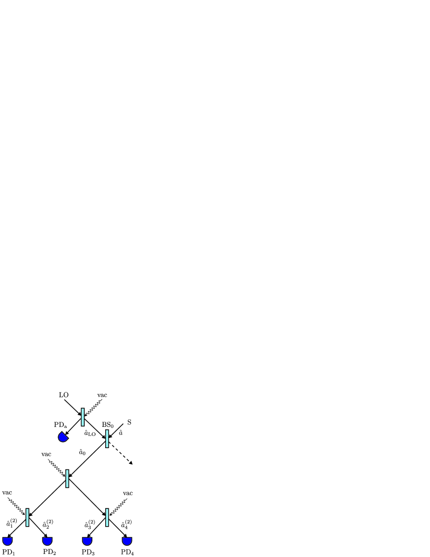
Figure 1: Scheme for measuring the moments $\langle(\hat{a}^{\dagger})^{k}\hat{a}^{l}\rangle$.

The entrance beam-splitter for the signal field, $\mathrm{BS_{0}}$, is characterized by the parameters $T_{0}$ and $R_{0}$ with

$$|T_{0}|\gg|R_{0}|,$$ (46)

so that the signal field of interest is almost completely used for the correlation measurements. In our scheme the strength of the local oscillator on the detectors is typically of the same order of magnitude as the signal field, which is easily realized with a weakly reflecting entrance beam splitter. All the other beam splitters in the device are $50$%-$50$%, so that their parameters $T_{k}$ and $R_{k}$ can be written in the simple form

$$T_{k}=\frac{1}{\sqrt{2}}e^{i\varphi_{k}},\quad R_{k}=\frac{i}{\sqrt{2}}e^{i\varphi_{k}}.$$ (47)

The operator $\hat{a}_{0}$ describing the field behind the entrance beam splitter $\mathrm{BS_{0}}$ reads as

$$\hat{a}_{0}=\frac{1}{\sqrt{2}}(T_{0}\hat{a}+R_{0}\hat{a}_{\mathrm{LO}}).$$ (48)

It is clear that all the operators $\hat{a}^{(d)}_{k}$, that describe the fields on the $k$-th detector, are proportional to the operator $\hat{a}_{0}$,

$$\hat{a}^{(d)}_{k}=\frac{e^{i\Phi_{k}}}{\sqrt{2^{d}}}\hat{a}_{0}+\ldots,$$ (49)

where $\ldots$ stands for a combination of the corresponding vacuum-channel operators which gives no contribution to the quantities considered below. The phase $\Phi_{k}$ depends on the path leading from the beam-splitter $\mathrm{BS_{0}}$ to the $k$-th photodetector $\mathrm{PD_{k}}$.

The measurement scheme can be used to detect the coincidences registered by all $n$ photodetectors, which are described by the normally-ordered correlation functions $\Gamma_{k_{1},\ldots,k_{n}}$ of the form

$$\Gamma_{k_{1},\ldots,k_{n}}=\langle:\hat{a}^{(d)\dagger}_{k_{1}}\hat{a}_{k_{1}}^{(d)}\ldots\hat{a}^{(d)\dagger}_{k_{n}}\hat{a}_{k_{n}}^{(d)}:\rangle.$$ (50)

Using Eq. (49) it is clear that these correlations do not depend on $k_{1},\ldots,k_{n}$ and they can be written as

$$\Gamma^{(n)}=\Gamma_{k_{1},\ldots,k_{n}}=\frac{1}{2^{nd}}\langle\hat{a}_{0}^{\dagger n}\hat{a}_{0}^{n}\rangle.$$ (51)

Summing up over all possible combinations of $n$ photo-detectors, in order to avoid loss of measured data, we get the following function:

$$\begin{split}F_{n}&=\sum_{\{k_{1},\ldots,k_{n}\}}\Gamma_{k_{1},\ldots,k_{n}}=\\ &\binom{2^{d}}{n}\Gamma^{(n)}=\sum^{n}_{m=-n}f_{n}(m)e^{im\varphi},\end{split}$$ (52)

where $\varphi=\varphi_{\mathrm{LO}}-\pi/2$ and the coefficients $f_{n}(m)$ read

$$\begin{split}f_{n}(m)=\frac{\binom{2^{d}}{n}}{2^{nd}}&\sum_{k-l=m}\binom{n}{k}\binom{n}{l}\times\\ &|T_{0}|^{k+l}|R_{0}\alpha|^{2n-k-l}\langle\hat{a}^{\dagger k}\hat{a}^{l}\rangle.\end{split}$$ (53)

The function $F_{n}$ in Eq. (52) is a function of the phase $\varphi$

$$F_{n}=F_{n}(\varphi),$$ (54)

and the coefficients $f_{n}(m)$ can be obtained from this function using Fourier transform

$$f_{n}(m)=\frac{1}{2\pi}\int_{0}^{2\pi}F_{n}(\varphi)e^{-im\varphi}\,d\varphi.$$ (55)

Each coefficient $f_{n}(m)$ in Eq. (53) is a combination of some moments $\langle\hat{a}^{\dagger k}\hat{a}^{l}\rangle$. From these combinations it is possible to extract the moments $\langle\hat{a}^{\dagger k}\hat{a}^{l}\rangle$ themselves step by step. The moments $\langle\hat{a}\rangle$, $\langle\hat{a}^{\dagger}\rangle$ and $\langle\hat{a}^{\dagger}\hat{a}\rangle$ can be obtained directly from $F_{1}(\varphi)$,

$$\begin{split}\langle\hat{a}\rangle&=\frac{f_{1}(-1)}{|T_{0}R_{0}\alpha|},\\ \langle\hat{a}^{\dagger}\rangle&=\frac{f_{1}(1)}{|T_{0}R_{0}\alpha|},\\ \langle\hat{a}^{\dagger}\hat{a}\rangle&=\frac{f_{1}(0)-|R_{0}\alpha|^{2}}{|T_{0}|^{2}}.\end{split}$$ (56)

Using these moments the next step gives the explicit expressions for the moments $\langle\hat{a}^{\dagger k}\hat{a}^{l}\rangle$, $k,l=1,2$. We present the expressions only for the moments $\langle\hat{a}^{2}\rangle$ and $\langle\hat{a}^{\dagger}\hat{a}^{2}\rangle$,

$$\begin{split}\langle\hat{a}^{2}\rangle&=\frac{8}{3}\frac{f_{2}(-2)}{|T_{0}R_{0}\alpha|^{2}},\\ \langle\hat{a}^{\dagger}\hat{a}^{2}\rangle&=\frac{1}{3}\frac{4f_{2}(-1)-3|R_{0}\alpha|^{2}f_{1}(-1)}{|T^{3}_{0}R_{0}\alpha|}.\end{split}$$ (57)

Figure 2 illustrates the possibility to extract the general moments $\langle\hat{a}^{\dagger k}\hat{a}^{l}\rangle$, $0\leqslant k,l\leqslant 2^{d}$ step by step. The $n$-th step is the extraction of the moments $\langle\hat{a}^{\dagger k}\hat{a}^{l}\rangle$ with $0\leqslant k,l\leqslant n$, i. e. the moments $\langle\hat{a}^{\dagger k}\hat{a}^{l}\rangle$ with $(k,l)$ corresponding to the square

$$S_{n}=\{(k,l)\in\mathbf{Z}^{2}|0\leqslant k,l\leqslant n\}.$$ (58)

But, in fact, we don’t measure the moments $\langle\hat{a}^{\dagger k}\hat{a}^{l}\rangle$ themselves, we measure their combinations $f_{n}(m)$, $m=-n,\ldots,n$, that consist of the moments $\langle\hat{a}^{\dagger k}\hat{a}^{l}\rangle$, $0\leqslant k,l\leqslant n$ with additional condition $k-l=m$. Geometrically the combination $f_{n}(m)$ contains the moments $\langle\hat{a}^{\dagger k}\hat{a}^{l}\rangle$ with $(k,l)$ in the intersection of the square $S_{n}$ and the inclined line $L_{m}:k-l=m$. This means that using the data obtained on one step only it is impossible to extract the moments $\langle\hat{a}^{\dagger k}\hat{a}^{l}\rangle$, but assuming we have the data of previous steps it is: each combination $f_{n+1}(m)$ contains one new moment by comparison with $f_{n}(m)$. Note that $f_{n+1}(n+1)$ and $f_{n+1}(-n-1)$ contain one moment only, $\langle\hat{a}^{\dagger n+1}\rangle$ and $\langle\hat{a}^{n+1}\rangle$ correspondingly, so that these moments can be measured without keeping the information of previous steps. Geometrically this means that $S_{n+1}\cap L_{m}$ contains one point more by comparison with $S_{n}\cap L_{m}$. So, step by step it is possible to extract all the moments $\langle\hat{a}^{\dagger k}\hat{a}^{l}\rangle$, $0\leqslant k,l\leqslant 2^{d}$. The last step, the $2^{d}$-th, consists in the extraction of the moments $\langle\hat{a}^{\dagger k}\hat{a}^{l}\rangle$ with $k$ or $l$ (or both) being equal to $2^{d}$.

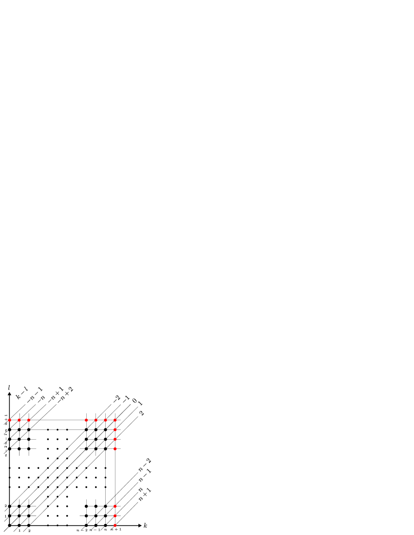
Figure 2: Step by step extraction of the moments $\langle\hat{a}^{\dagger k}\hat{a}^{l}\rangle$.

III.2 Detection of $\langle:\hat{x}_{\varphi}^{k}\hat{p}_{\varphi}^{l}:\rangle$

The moments $\langle:\hat{x}_{\varphi}^{k}\hat{p}_{\varphi}^{l}:\rangle$ can be measured with the scheme presented on the Fig. 3, as it has been proposed in Shchukin et al. (2005). In fact, this is a slightly modified version of the Noh-Fougères-Mandel device Noh et al. (1991). The lowest-order moments are explicitely expressed in terms of the correlation functions $\Gamma_{j}$, $\Gamma_{jk}$ according to the following formulas:

$$\langle\hat{x}_{\varphi}\rangle=\sqrt{2}\frac{\Gamma_{3}-\Gamma_{4}}{|\alpha|},\quad\langle\hat{p}_{\varphi}\rangle=\sqrt{2}\frac{\Gamma_{1}-\Gamma_{2}}{|\alpha|}.$$ (59)

The second-order moments are of the form

$$\begin{split}\langle:\hat{x}_{\varphi}^{2}:\rangle&=4\frac{\Gamma_{12}-\Gamma_{34}}{|\alpha|^{2}}+\langle\hat{n}\rangle,\\ \langle:\hat{p}_{\varphi}^{2}:\rangle&=4\frac{\Gamma_{34}-\Gamma_{12}}{|\alpha|^{2}}+\langle\hat{n}\rangle,\\ \langle:\hat{x}_{\varphi}\hat{p}_{\varphi}:\rangle&=4\frac{\Gamma_{13}+\Gamma_{24}-\Gamma_{12}-\Gamma_{34}}{|\alpha|^{2}}-\langle\hat{n}\rangle,\end{split}$$ (60)

where

$$\langle\hat{n}\rangle=\Gamma_{1}+\Gamma_{2}+\Gamma_{3}+\Gamma_{4}-|\alpha|^{2}.$$ (61)

The amplitude $|\alpha|$ of the local oscillator is detected by the auxiliary photodetector $\mathrm{PD}_{\mathrm{a}}$. Note that one could also try to use the measured data more efficiently as discussed in detail in the preceding subsection. However, this would lead to somewhat more complex expressions for the moments. Since the procedure is straightforward, we do not present it here.

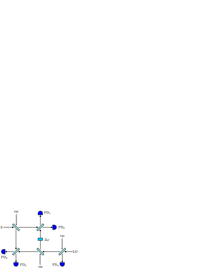
Figure 3: Scheme for measuring the moments $\langle:\hat{x}_{\varphi}^{k}\hat{p}_{\varphi}^{l}:\rangle$.

The scheme in the form shown in Fig. 3 allows one to determine all the moments $\langle:\hat{x}^{k}_{\varphi}\hat{p}^{l}_{\varphi}:\rangle$ up to the order of $k+l=4$. The further extension of the method is straightforward. For example, each of the detectors $\mathrm{PD}_{i}$ ($i=1\ldots 4$) can be replaced with a beam splitter, each of which mixing the field with a vacuum input. In their output ports the output fields are detected by pairs of photodetectors. This allows us to extract the moments up to the order of $k+l=8$, and so forth.

III.3 Detection of $\langle:\hat{x}_{\varphi}^{k}\hat{n}^{l}:\rangle$

Figure 4 illustrates the possibility of measuring moments $\langle:\hat{x}_{\varphi}^{k}\hat{n}^{l}:\rangle$ by an extended version of the homodyne cross correlation scheme considered in Ref. Vogel (1995). The moments $\langle\hat{n}\rangle$ and $\langle\hat{x}_{\varphi}\rangle$ can be obtained according to the following relations

$$\begin{split}\langle\hat{n}\rangle&=\Gamma_{1}+\Gamma_{2}+\Gamma_{3}+\Gamma_{4}-|\alpha|^{2},\\ \langle\hat{x}_{\varphi}\rangle&=\frac{1}{|\alpha|^{2}}\Bigl{(}\Gamma_{1}+\Gamma_{2}-\Gamma_{3}-\Gamma_{4}\Bigr{)}.\end{split}$$ (62)

Higher-order moments can be extracted from the measured data step by step.

We give explicit expressions only for the second-order moments. The moment $\langle:\hat{n}^{2}:\rangle$ can be directly measured with blocked local oscillator. Note that this moment and the first-order moments together allow one to calculate the moment $\langle:\hat{x}_{\varphi}^{2}:\rangle$:

$$\begin{split}\Gamma_{13}&+\Gamma_{14}+\Gamma_{23}+\Gamma_{24}=\\ &\frac{1}{4}\Bigl{(}\langle:\hat{n}^{2}:\rangle+2|\alpha|^{2}\langle\hat{n}\rangle+|\alpha|^{4}-|\alpha|^{2}\langle:\hat{x}_{\varphi}^{2}:\rangle\Bigr{)}.\end{split}$$ (63)

The moment $\langle:\hat{n}\hat{x}_{\varphi}:\rangle$ can be obtained from the simple relation

$$\Gamma_{12}-\Gamma_{34}=\frac{1}{4}\Bigl{(}|\alpha|\langle:\hat{n}\hat{x}_{\varphi}:\rangle+|\alpha|^{2}\langle\hat{x}_{\varphi}\rangle\Bigr{)}.$$ (64)

All higher-order moments can be measured in such a way with an appropriately extended version of the scheme shown in Fig. 4.

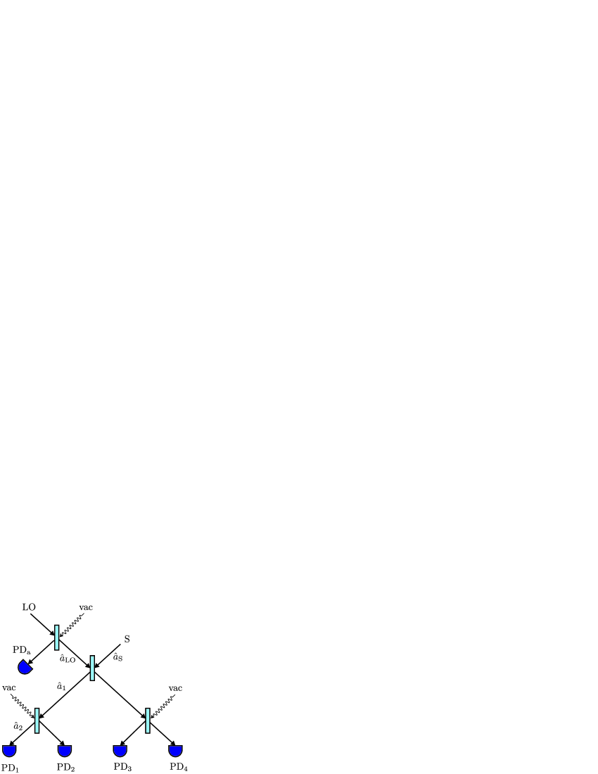
Figure 4: Scheme for measuring the moments $\langle:\hat{x}_{\varphi}^{k}\hat{n}^{l}:\rangle$.

IV Amplitude-squared squeezing

In this section we will consider a particular nonclassical effect which can be well described in terms of the moments-based nonclassicality criteria derived in Sec. II. The examples will also be simple from the viewpoint of the measurement of the needed moments, when the measurement principles of Sec. III are used. This example is the amplitude squared squeezing Hillery (1987). We note that for the measurement of amplitude-squared squeezing to our knowledge there exists no direct measurement principle. It has been proposed to measure the effect after the interaction with a Kerr medium Hillery (1991). Such techniques are, however, not easy to use and require sufficiently strong signal fields for realizing the nonlinear interaction before the detection. Hence a possibility of a more direct measurement of the effect would be of interest.

Let us start with the characterization of the nonclassical effects we are interested in. As a special choice of $\hat{f}$ in the nonclassicality condition (9) let us consider the following operator

$$\hat{X}_{\varphi}=\hat{a}^{2}e^{i\varphi}+\hat{a}^{\dagger 2}e^{-i\varphi}.$$ (65)

According to (8) for any number $c$ the mean value

$$\langle:(\hat{X}_{\varphi}-c)^{2}:\rangle\geqslant 0$$ (66)

is nonnegative for all classical states. For $c=\langle\hat{X}_{\varphi}\rangle$ this gives the following condition:

$$\langle:(\Delta\hat{X}_{\varphi})^{2}:\rangle\geqslant 0,$$ (67)

or, in other words, the condition

$$\langle:(\Delta\hat{X}_{\varphi})^{2}:\rangle<0$$ (68)

is sufficient for nonclassicality. We note that the condition for amplitude-squared squeezing can be easily expressed as

$$s^{(2)}_{\varphi}=\begin{vmatrix}1&\langle:\hat{x}_{\varphi}\hat{p}_{\varphi}:\rangle\\[2.15277pt] \langle:\hat{x}_{\varphi}\hat{p}_{\varphi}:\rangle&\langle:\hat{x}_{\varphi}^{2}\hat{p}^{2}_{\varphi}:\rangle&\end{vmatrix}<0,$$ (69)

in terms of the moments of two quadratures.

Another way to formulate the condition for amplitude-squared squeezing is based on the moments of the operators $\hat{a}^{\dagger}$, $\hat{a}$. Let us consider the subdeterminant $s_{3}$ that results from the determinant (12) by canceling all its rows and columns except those beginning with the elements $1$, $\langle\hat{a}^{2}\rangle$ and $\langle\hat{a}^{\dagger 2}\rangle$. This leads to a nonclassicality condition of the form

$$s_{3}=\begin{vmatrix}1&\langle\hat{a}^{\dagger 2}\rangle&\langle\hat{a}^{2}\rangle\\ \langle\hat{a}^{2}\rangle&\langle\hat{a}^{\dagger 2}\hat{a}^{2}\rangle&\langle\hat{a}^{4}\rangle\\ \langle\hat{a}^{\dagger 2}\rangle&\langle\hat{a}^{\dagger 4}\rangle&\langle\hat{a}^{\dagger 2}\hat{a}^{2}\rangle\end{vmatrix}<0.$$ (70)

We show that the negativity of this determinant is equivalent to the following condition

$$\Bigl{\langle}:(\Delta\hat{X}_{\varphi})^{2}:\Bigr{\rangle}<0,\quad\forall\varphi.$$ (71)

In fact, the determinant (70) can be written as follows:

$$s_{3}=\frac{1}{4}\min_{\varphi}\Bigl{\langle}:(\Delta\hat{X}_{\varphi})^{2}:\Bigr{\rangle}\max_{\varphi}\Bigl{\langle}:(\Delta\hat{X}_{\varphi})^{2}:\Bigr{\rangle}.$$ (72)

It is not difficult to see that the last term in the product on the right hand side of this equality is always nonnegative

$$\max_{\varphi}\Bigl{\langle}:(\Delta\hat{X}_{\varphi})^{2}:\Bigr{\rangle}\geqslant 0.$$ (73)

The explicit expressions for the minimum and the maximum of the variance of the operator $\hat{X}_{\varphi}$ are

$$\begin{split}\min_{\varphi}\Bigl{\langle}:(\Delta\hat{X}_{\varphi})^{2}:\Bigr{\rangle}&=2\Bigl{[}\Bigl{\langle}\Delta\hat{a}^{\dagger 2}\Delta\hat{a}^{2}\Bigr{\rangle}-\Bigl{|}\Bigl{\langle}(\Delta\hat{a}^{2})^{2}\Bigr{\rangle}\Bigr{|}\Bigr{]},\\ \max_{\varphi}\Bigl{\langle}:(\Delta\hat{X}_{\varphi})^{2}:\Bigr{\rangle}&=2\Bigl{[}\Bigl{\langle}\Delta\hat{a}^{\dagger 2}\Delta\hat{a}^{2}\Bigr{\rangle}+\Bigl{|}\Bigl{\langle}(\Delta\hat{a}^{2})^{2}\Bigr{\rangle}\Bigr{|}\Bigr{]}.\end{split}$$ (74)

It is clear that the mean value $\Bigl{\langle}\Delta\hat{a}^{\dagger 2}\Delta\hat{a}^{2}\Bigr{\rangle}$ is always nonnegative. Due to the second of the equalities (74) the maximal variance of $\hat{X}_{\varphi}$ is always nonnegative. Hence the condition for the negativity of $s_{3}$ in Eq. (72) is a direct demonstration of amplitude-squared squeezing.

An advantage of this method for demonstrating amplitude squared squeezing consists in the fact that we do not need to adjust the local oscillator phase to the noise minimum. The negativity of the considered subdeterminant demonstrates the negativity of the minimum of the normally-ordered variance already. Moreover, the moments $\langle\hat{a}^{2}\rangle$, $\langle\hat{a}^{4}\rangle$ and $\langle\hat{a}^{\dagger 2}\hat{a}^{2}\rangle$ needed in the condition (70) are easily obtained by the methods of the preceding section.

V minimum-uncertainty amplitude-squared squeezed states

Let us consider amplitude squared-squeezed states in more detail (Hillery (1987); Bergou et al. (1991); Yu and Hillery (1994)). By definition, a state is amplitude-squared squeezed if

$$\min_{\varphi}\langle:(\Delta\hat{X}_{\varphi})^{2}:\rangle<0,$$ (75)

which can be rewritten in the equivalent form as

$$\exists\varphi:\quad\langle(\Delta\hat{X}_{\varphi})^{2}\rangle<4\langle\hat{n}\rangle+2.$$ (76)

We consider here a special class of amplitude-squared squeezed states that satisfy the minimum uncertainty relation Bergou et al. (1991). For this purpose we introduce the operators

$$\hat{X}=\hat{X}_{\varphi},\quad\hat{Y}=\hat{X}_{\varphi+\pi/2}.$$ (77)

They fulfill the uncertainty relation

$$\langle(\Delta\hat{X})^{2}\rangle^{1/2}\langle(\Delta\hat{Y})^{2}\rangle^{1/2}\geqslant 4\langle\hat{n}\rangle+2.$$ (78)

A state satisfies the minimum uncertainty relation if

$$\langle(\Delta\hat{X})^{2}\rangle^{1/2}\langle(\Delta\hat{Y})^{2}\rangle^{1/2}=4\langle\hat{n}\rangle+2.$$ (79)

In the following we will only consider pure quantum states.

As it has been shown in Yu and Hillery (1994), a pure state $|\psi\rangle$ satisfies the condition (79) if it is a solution of the eigenvalue problem

$$(\hat{X}+i\lambda\hat{Y})|\psi\rangle=\beta|\psi\rangle,$$ (80)

for all real nonnegative $\lambda$ and any complex $\beta$. One can easily check that form Eq. (80) it follows that

$$\begin{split}\langle(\Delta\hat{X})^{2}\rangle&=\lambda(4\langle\hat{n}\rangle+2),\\ \langle(\Delta\hat{Y})^{2}\rangle&=\frac{1}{\lambda}(4\langle\hat{n}\rangle+2).\end{split}$$ (81)

For either $\lambda>1$ or $1/\lambda>1$ one of the variations on the left-hand sides of Eqs (81) satisfies the condition (76). Therefore the state (80) is always amplitude-square squeezed, except for $\lambda=1$.

(a) $\lambda=1.01$

(b) $\lambda=1.05$

(c) $\lambda=1.1$

(d) $\lambda=2$

Figure 5: The $Q$ function of amplitude square squeezed states (82) for $m=2$.

It was shown in Bergou et al. (1991) that there exist solutions of Eq. (80) of the form

$$|\psi(m,\lambda)\rangle=c_{m}(\lambda)\hat{S}(z)H_{m}(i\gamma\hat{a}^{\dagger})|0\rangle,$$ (82)

where

$$\gamma=\gamma(\lambda)=\begin{cases}e^{i\pi/4}\sqrt{\sqrt{1-\lambda^{2}}/2}&0<\lambda<1,\\ \sqrt{\sqrt{\lambda^{2}-1}/{2\lambda}}&1<\lambda,\end{cases}$$ (83)

and

$$|c_{m}(\lambda)|^{2}=\begin{cases}1&m=0,\\ \frac{(-1)^{m}}{m!C^{-m}_{m}(2|\gamma(\lambda)|^{2})}&m>0.\end{cases}$$ (84)

The parameter $\beta$ in the equation (80) is connected with $m$ and $\lambda$ by the expression

$$\beta=\begin{cases}i\sqrt{1-\lambda^{2}}(2m+1)&0<\lambda<1,\\ \sqrt{\lambda^{2}-1}(2m+1)&1<\lambda.\end{cases}$$ (85)

The parameter $z=z(\lambda)=re^{i\varphi}$ reads

$$\tanh^{2}r=\frac{\lambda-1}{\lambda+1}e^{-2i\varphi},\quad\varphi=\begin{cases}\pi/2&0<\lambda<1,\\ 0&1<\lambda.\end{cases}$$ (86)

Some examples of the $Q$-function of the states (82) are shown in Fig. 5.

In Fig. 6 we illustrate examples of the determinants for the minimum-uncertainty amplitude-squared squeezed states under study. It is of great importance that all the moments appearing in the nonclassicality condition (70) can be determined by the homodyne correlation measurement technique proposed in Sec. III.1. Unless the methods of quantum-state reconstruction, for a review cf. Welsch et al. (1999), the measurements proposed here are even possible in cases when the overall quantum efficiency of the detection device is small.

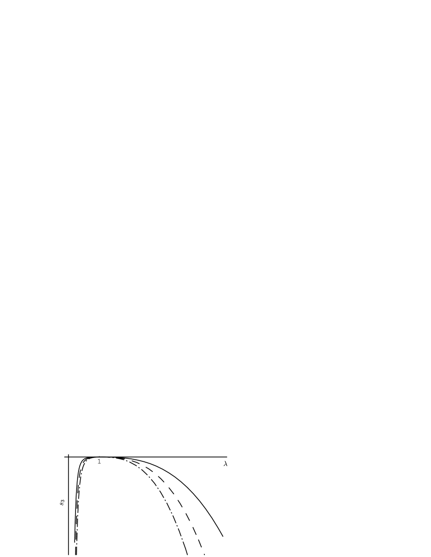
Figure 6: The determinants $s_{3}$ (70) for $m=2$ (solid), $m=3$ (dashed) and $m=4$ (dash-dotted).

VI Summary and Conclusion

We have shown that condition for the nonclassicality of a single-mode quantum state, that is the failure of the $P$-function to be a probability measure, can be formulated in different ways. All the versions of necessary and sufficient conditions the we have formulated in this paper turn out to be special representations of the violation of Bochner’s condition for the existence of a classical characteristic function of the $P$-function. The considered formulations of different forms of nonclassicality criteria include characteristic functions of quadratures and different types of normally-ordered moments. Most importantly, all the quantities under study are accessible to observation. Their measurement, however, requires to develop new types of measurement principles.

We have proposed rather simple and direct methods of measuring three kinds of normally-ordered moments of a single-mode radiation field. For each type of moments a particular detection scheme is analyzed: for the moments $\langle\hat{a}^{\dagger k}\hat{a}^{l}\rangle$ of the creation and annihilation operators, the moments $\langle:\hat{x}^{k}_{\varphi}\hat{p}^{l}_{\varphi}:\rangle$ of two quadratures and the moments $\langle:\hat{x}^{k}_{\varphi}\hat{n}^{l}:\rangle$ of a quadrature and the photon number operator. In all the considered schemes the total number $N$ of photo-detectors needed to measure these moments is at most twice as large as the largest value of $k$ and $l$: $N<2\max(k,l)$. We also tried to present the extraction procedure for the moments in an optimal way form the viewpoint of an effective use of the available measured data. This means that one tries to use all the data obtained in measurements. Unfortunately this does not provide the expressions for the moments of interest in its simplest form. In the simplest form one would not need to sum up the correlation functions of all possible combinations of photo-detectors to get the moments. However, one would lose part of the measured data and thus this simplified approach would be less precise from the experimental point of view.

Our new methods of characterizing nonclassical effects by moments of annihilation and creation operators are applied to the characterization of amplitude-squared squeezing. We have shown that our criteria give a direct insight in the effect of amplitude-squared squeezing without the need of adjusting the phase of the local oscillator. More importantly, the demonstration of amplitude-squared squeezing until now was considered to require a rather difficult and indirect observation procedure, so that this effect received little attention in the context of experiments. The measurement procedures proposed in this paper turn out to be of particular simplicity for demonstrating the amplitude-squared squeezing effect. This may lead to new interest in this special nonclassical effect.

In conclusion we have formulated new types of criteria for characterizing nonclassical effects of radiation fields. For all versions of nonclassicality criteria we have proposed appropriate and simple measurement principles. These principles are based on homodyne correlation techniques with a weak local oscillator. They can be used even when the quantum efficiency of the device is small. The proposed methods may open new possibilities of demonstration and practical application of nonclassical effects of radiation fields.

*

Appendix A Moments of amplitude-squared squeezed states

The moments $\langle\hat{a}^{\dagger k}\hat{a}^{l}\rangle_{m}$ of the state $|\psi_{m}\rangle$ can be obtained in the following way. Let us take

$$|\tilde{\psi}_{m}\rangle=c^{-1}_{m}|\psi_{m}\rangle=\hat{S}(z)H_{m}(i\gamma\hat{a}^{\dagger})|0\rangle,$$ (87)

where the parameters $z$ and $\gamma$ are defined by the Eqs. (86) and (83) correspondingly. It is clear that

$$\langle\hat{a}^{\dagger k}\hat{a}^{l}\rangle_{m}=\langle\tilde{\psi}_{m}|\hat{a}^{\dagger k}\hat{a}^{l}|\tilde{\psi}_{m}\rangle.$$ (88)

We calculate the quantities $\langle\tilde{\psi}_{m}|\hat{a}^{\dagger k}\hat{a}^{l}|\tilde{\psi}_{m}\rangle$ with the help of the generating function

$$F(x,y,u,v)=\sum^{+\infty}_{n,m,k,l=0}\langle\tilde{\psi}_{n}|\hat{a}^{\dagger k}\hat{a}^{l}|\tilde{\psi}_{m}\rangle\frac{x^{n}y^{m}u^{k}v^{l}}{n!m!k!l!}.$$ (89)

Clearly,

$$\begin{split}\sum^{+\infty}_{n,m=0}&\langle\tilde{\psi}_{n}|\hat{a}^{\dagger k}\hat{a}^{l}|\tilde{\psi}_{m}\rangle\frac{x^{n}y^{m}}{n!m!}=\\ &\langle 0|e^{-x^{2}-2i\overline{\gamma}x\hat{a}}\hat{S}^{\dagger}(z)\hat{a}^{\dagger k}\hat{a}^{l}\hat{S}(z)e^{-y^{2}+2i\gamma y\hat{a}^{\dagger}}|0\rangle,\end{split}$$ (90)

and the function $F(x,y,u,v)$ reads as

$$\begin{split}&F(x,y,u,v)=\\ &\langle 0|e^{-x^{2}-2i\overline{\gamma}x\hat{a}}\hat{S}^{\dagger}(z)e^{u\hat{a}^{\dagger}}e^{v\hat{a}}\hat{S}(z)e^{-y^{2}+2i\gamma y\hat{a}^{\dagger}}|0\rangle.\end{split}$$ (91)

Using the relation

$$\hat{a}\hat{S}(z)=\hat{S}(z)(\mu\hat{a}+\nu\hat{a}^{\dagger})$$ (92)

it can be further simplified to the following form

$$F(x,y,u,v)=\exp\Bigl{(}-\frac{1}{2}\mathbf{w}^{T}A\mathbf{w}\Bigr{)},$$ (93)

where $\mathbf{w}=(x,y,u,v)^{T}$ and

$$A=\begin{pmatrix}2&-4|\gamma|^{2}&-2i\overline{\nu}\gamma&-2i\mu\gamma\\ -4|\gamma|^{2}&2&2i\mu\overline{\gamma}&2i\nu\overline{\gamma}\\ -2i\overline{\nu}\gamma&2i\mu\overline{\gamma}&-\mu\overline{\nu}&-|\nu|^{2}\\ -2i\mu\gamma&2i\nu\overline{\gamma}&-|\nu|^{2}&-\mu\nu\end{pmatrix}.$$ (94)

From this expression it follows that

$$\langle\tilde{\psi}_{n}|\hat{a}^{\dagger k}\hat{a}^{l}|\tilde{\psi}_{m}\rangle=H^{\{A\}}_{nmkl}(0,0,0,0),$$ (95)

where $H^{\{A\}}_{nmkl}(0,0,0,0)$ is a four-dimensional Hermite polynomial defined as ($\mathbf{e}=(a,b,c,d)^{T}$)

$$\begin{split}\sum^{+\infty}_{n,m,k,l=0}&H^{\{A\}}_{nmkl}(a,b,c,d)\frac{x^{n}y^{m}u^{k}v^{l}}{n!m!k!l!}=\\ &\exp\left(-\frac{1}{2}\mathbf{w}^{T}A\mathbf{w}+\mathbf{w}^{T}A\mathbf{e}\right).\end{split}$$ (96)

Finally, we arrive at the result

$$\langle\hat{a}^{\dagger k}\hat{a}^{l}\rangle_{m}=|c_{m}|^{2}H^{\{A\}}_{mmkl}(0,0,0,0),$$ (97)

for the moments we are interested in.

References

- Kimble et al. (1977) H. J. Kimble, M. Dagenais, and L. Mandel, Phys. Rev. Lett. 39, 691 (1977).
- Short and Mandel (1983) R. Short and L. Mandel, Phys. Rev. Lett. 51, 384 (1983).
- Slusher et al. (1985) R. Slusher, L. Hollberg, B. Yurke, J. Mertz, and J. Valley, Phys. Rev. Lett. 55, 2409 (1985).
- Smithey et al. (1993) D. T. Smithey, M. Beck, M. G. Raymer, and A. Faridani, Phys. Rev. Lett. 70, 1244 (1993).
- Welsch et al. (1999) D.-G. Welsch, W. Vogel, and T. Opatrný, Homodyne detection and quantum-state reconstraction (Elsevier science B. V., 1999), vol. 39 of Progress in Optics, chap. 2, pp. 63–211.
- Vogel (1991) W. Vogel, Phys. Rev. Lett. 67, 2450 (1991).
- Vogel (1995) W. Vogel, Phys. Rev. A 51, 4160 (1995).
- Carmichael et al. (2000) H. J. Carmichael, H. M. Castro-Beltran, G. T. Foster, and L. A. Orozco, Phys. Rev. Lett. 85, 1855 (2000).
- Beck et al. (2001) M. Beck, C. Dorrer, and I. A. Walmsley, Phys. Rev. Lett. 87, 253601 (2001).
- Titulaer and Glauber (1965) U. Titulaer and R. Glauber, Phys. Rev. 140, B676 (1965).
- Mandel (1986) L. Mandel, Phys. Scr. T12, 34 (1986).
- Vogel (2000) W. Vogel, Phys. Rev. Lett. 84, 1849 (2000).
- Johansen (2004) L. M. Johansen, Phys. Lett. A 329, 184 (2004).
- Johansen and Luis (2004) L. M. Johansen and A. Luis, Phys. Rev. A 70, 052115 (2004).
- Lvovsky and Shapiro (2002) A. Lvovsky and J. H. Shapiro, Phys. Rev. A 65, 033830 (2002).
- Richter and Vogel (2002) T. Richter and W. Vogel, Phys. Rev. Lett. 89, 283601 (2002).
- Bochner (1933) S. Bochner, Math. Ann. 108, 378 (1933).
- Kawata (1972) T. Kawata, Fourier Analysis in Probability Theory (Academic Press, New York, 1972).
- Shchukin et al. (2005) E. Shchukin, T. Richter, and W. Vogel, Phys. Rev. A 71, 011802 (2005).
- Agarwal and Tara (1992) G. Agarwal and K. Tara, Phys. Rev. A 46, 485 (1992).
- Agarwal (1993) G. Agarwal, Opt. Commun. 95, 109 (1993).
- Klyshko (1996) D. N. Klyshko, Physics-Uspekhi 39, 573 (1996).
- Korbicz et al. (2005) J. K. Korbicz, J. I. Cirac, J. Wehr, and M. Lewenstein, Phys. Rev. Lett. 94, 153601 (2005).
- Asbóth et al. (2005) J. K. Asbóth, J. Calsamiglia, and H. Ritsch, Phys. Rev. Lett. 94, 173602 (2005).
- Hillery (1987) M. Hillery, Phys. Rev. A 36, 3796 (1987).
- Sudarshan (1963) E. Sudarshan, Phys. Rev. Lett. 10, 277 (1963).
- Glauber (1963) R. J. Glauber, Phys. Rev. 131, 2766 (1963).
- Prestel and Delzell (2001) A. Prestel and C. N. Delzell, Positive Polynomials: From Hilbert’s 17th Problem to Real Algebra (Springer, Berlin Heidelberg, 2001).
- Noh et al. (1991) J. W. Noh, A. Fougères, and L. Mandel, Phys. Rev. Lett. 67, 1426 (1991).
- Hillery (1991) M. Hillery, Phys. Rev. A 44, 4578 (1991).
- Bergou et al. (1991) J. A. Bergou, M. Hillery, and D. Yu, Phys. Rev. A 43, 515 (1991).
- Yu and Hillery (1994) D. Yu and M. Hillery, Quantum. Opt. 6, 37 (1994).