Entanglement of bosonic modes in symmetric graphs
M. Asoudeh,       V. Karimipour

Department of Physics, Sharif University of Technology,

P.O. Box 11365-9161,

Tehran, Iran

The ground and thermal states of a quadratic hamiltonian representing the interaction of bosonic modes or particles are always Gaussian states. We investigate the entanglement properties of these states for the case where the interactions are represented by harmonic forces acting along the edges of symmetric graphs, i.e. 1, 2, and 3 dimensional rectangular lattices, mean field clusters and platonic solids. We determine the Entanglement of Formation (EoF) as a function of the interaction strength, calculate the maximum EoF in each case and compare these values with the bounds found in [1] which are valid for any quadratic hamiltonian.

PACS Numbers: 03.67.-a, 03.65.Bz, 03.67.Hk

1 Introduction

Suppose we have a many body quantum system in its ground state. We ask how much quantum correlation or entanglement exists between two of the particles? How this entanglement depends on the strength of interaction between the particles? Does it extend far beyond the nearest neighbor particles? If we raise the temperature, hence mixing the ground state with higher level states, at what temperature the entanglement ceases to exist? Some of these questions have been investigated in recent years for spin systems [2, 3, 4, 5, 6, 7, 8]. Quite recently another class of systems composed of bosonic modes of systems with continuous degrees of freedom have come under intensive investigations [9, 10, 11, 12, 13, 14, 15, 16, 17, 18]. There are a number of reasons for this interest. First, bosonic modes are the appropriate subsystems the entanglement of which must be calculated when dealing with systems of identical boson particles [19, 20, 21, 22]. Second, states of continuous systems are widely encountered in many branches of physics in which entanglement plays a role, i.e. namely in quantum optical setups, in atomic ensembles interacting with electromagnetic fields [9], in the motion of ions in ion traps and in low excitations of bosonic field theories. Third, for a class of such states, namely Gaussian states, analytical measures of entanglement have been defined and calculated in closed form [15]. Finally, a large class of interesting many body systems of this type, when written in terms of suitable coordinates, are in fact free systems. This latter reason makes a fuller investigation of the above questions in such systems much easier than in spin systems. For example it has been shown [12] that in the ground state of a ring of particles coupled with each other by harmonic forces, entanglement exists only between adjacent particles and is exactly zero if the particles are non-adjacent. It has also been possible to study the development of entanglement when such systems evolve in time [13]. Neither of these questions are easy to investigate in spin systems.
Furthermore quite interestingly the notion of entanglement frustration has recently been introduced in [1]. The motivation for this notion comes from the observation that quantum entanglement like many other local properties of a system becomes strongly restricted when one imposes global symmetry requirements on the state of a system of $N$ particles. For example the Entanglement of Formation (EoF)[15] of two modes in a Gaussian state is generally unbounded, it can assume any value between zero and infinity. However if these modes are part of a three mode system having a permutation symmetry, then the amount of their EoF becomes finite. Therefore one may ask how the EoF of two modes in a system, may depend on the total number of modes, the symmetry of the state and the dimension of the lattice which represents the interaction of these modes. These questions have been studied in [1], with the aim of determining the maximum value of EoF which can exist between two modes given that the whole state has a general symmetry. However the Hamiltonian of [1] is a specific hamiltonian having no tunable parameter(i.e. frequencies), in fact it has been so defined that its ground state allows the maximum value of EoF among all the possible quadratic Hamiltonians with the same symmetry.

In this paper we want to study the effect of interaction strength and symmetry in determining the entanglement of bosonic modes in a class of states pertaining to the ground state of symmetric graphs. We take a system of $N$ particles or bosonic modes coupled quadratically with each other so that the Hamiltonian allows a global symmetry. We then determine the entanglement of two modes when the system is in its ground state. The entanglement depends on the number of particles, the strength of interaction and the symmetry of the Hamiltonian. We will see that entanglement always increases (almost rapidly) with the strength of interaction and always saturates to a finite limiting value but does not exceed the bounds found in [1]. We also show that in some cases symmetry has a constructive effect on entanglement. For example in some symmetric graphs like a cube or an octahedron, there are entanglement between next-nearest neighbors which is known to be absent in less symmetric graphs, i.e. in rings [12]. In the most simple case, where the graph consists of two vertices connected by an edge, we also calculate the thermal entanglement as a function of temperature and interaction strength and determine the threshold temperature beyond which entanglement vanishes.
The structure of this paper is as follows: In section 2 we review briefly the definition of Gaussian states and the Entanglement of Formation (EoF) for symmetric two-mode Gaussian states. In section 3 we introduce the quadratic Hamiltonian and calculate the EoF of two Gaussian modes when the whole system is in the ground state of this quadratic hamiltonian. This hamiltonian simply describes a mass-spring system of the kind considered in [12] and is different from the one introduced in [1], which maximizes the EoF. In section 4 we present our results for various symmetric graphs. We end the paper with a conclusion. A remark on notation. Throughout the paper we use $E_{inf}$ for the maximum EoF which is obtained at infinite frequencies (interaction strength of the springs) in our hamiltonian and $E_{max}$ for the bound discovered in [1].

2 Gaussian States

In this section we discuss the rudimentary material on Gaussian states [23] that we need in the sequel. Reference [24] can be consulted for a rather detailed review on the subject of Gaussian states.
Let $\hat{R}:=(\hat{x}_{1},\hat{x}_{2},\cdots\hat{x}_{N},\hat{p}_{1},\hat{p}_{2},\cdots\hat{p}_{N})$ be $N$ conjugate operators characterizing $N$ modes and subject to the canonical commutation relations

$$[\hat{R}_{k},\hat{R}_{l}]=i\sigma_{kl},$$

where $\sigma=\left(\begin{array}[]{cc}&I_{n}\\ -I_{n}&\end{array}\right)$ is the $2n$ dimensional symplectic matrix and $I_{n}$ denotes the $n$ dimensional unit matrix.
A quantum state $\rho$ is called Gaussian if its characteristic function defined as

$$C(\xi):=tr(e^{-i\xi_{k}\sigma_{kl}\hat{R}_{l}}\rho),$$

is a Gaussian function of the $\xi$ variables, namely if

$$C(\xi):=e^{\frac{-1}{2}\xi_{k}\Gamma_{kl}\xi_{l}},$$

where we have assumed that linear terms have been removed by suitable unitary transformations. The matrix $\Gamma$, called the covariance matrix of the state, encodes all the correlations in the form

$$\Gamma_{kl}:=\langle R_{k}R_{l}+R_{l}R_{k}\rangle-2\langle R_{k}\rangle\langle R_{l}\rangle.$$

By symplectic transformations the covariance matrix of a two mode symmetric Gaussian state (one which is invariant under the interchange of the two modes) can always be put into the standard form

$$\gamma=\left(\begin{array}[]{cccc}n&k_{x}&&\\ k_{x}&n&&\\ &&n&k_{p}\\ &&k_{p}&n\end{array}\right),$$ (1)

where $k_{x}\geq 0\geq k_{p}$ and $k_{x}\geq|k_{p}|$. For such a state the Entanglement of Formation (EoF) has been obtained in [15]. It is given by

$$EoF(\rho):=C_{+}\log_{2}C_{+}-C_{-}\log_{2}C_{-},$$ (2)

in which

$$C_{\pm}=\frac{(1\pm\Delta)^{2}}{4\Delta},$$ (3)

and

$$\Delta:=min(1,\delta:=\sqrt{(n-k_{x})(n+k_{p})}).$$ (4)

Thus a state is entangled only if $\delta\leq 1$. In general $EoF$ is unbounded and can assume any value between $0$ for $\delta=1$ to infinity for $\delta\longrightarrow 0$.

3 The ground and thermal entanglement of a system of particles coupled by harmonic forces

Consider now a system of particles with canonical variables $R=(x_{1},x_{2},\cdots x_{N},p_{1},p_{2},\cdots p_{N})^{T}$ subject to the following Hamiltonian

$$H=\frac{1}{2}\sum_{k=1}^{N}{p_{k}^{2}}+\frac{1}{2}\sum_{k=1}^{N}x_{k}^{2}+\frac{1}{2}\omega^{2}\sum^{\prime}_{k,l}(x_{k}-x_{l})^{2},$$ (5)

where the prime over the sum indicates that only specific particles are coupled with each other. This Hamiltonian can be written in matrix form

$$H=\frac{1}{2}R^{T}\left(\begin{array}[]{cc}\hat{V}&0\\ 0&I\end{array}\right)R,$$ (6)

where $\hat{V}$ introduces the quadratic matrix of the potential. The state of such a system at temperature $T=\frac{1}{\beta}$ is given by $\rho=\frac{e^{-\beta H}}{Z}$, where $Z=tre^{-\beta H}$ is the partition function. It is not difficult to show that this state is Gaussian [12] with covariance matrix

$$\Gamma = \Gamma_{x}\oplus\Gamma_{p},$$ (7)

$$\Gamma_{x} = W^{-1}\coth\frac{\beta W}{2},$$ (8)

$$\Gamma_{p} = W\coth\frac{\beta W}{2},$$ (9)

where $W:=V^{\frac{1}{2}}$. At zero temperature when only the ground state is populated the covariance matrix tends to

$$\Gamma(T=0)=W^{-1}\oplus W.$$ (10)

Once the covariance matrix of the $N$ modes is obtained as above, the covariance matrix pertaining to any two modes, say the modes $1$ and $2$ is given by the sub-matrix obtained from $\Gamma$ by deleting the rows and columns corresponding to all the other modes. Furthermore if this Gaussian state is symmetric, i.e. if it is invariant under the interchange of the two modes, then its covariance matrix will have the following (not-yet standard) form

$$\gamma=\left(\begin{array}[]{cccc}n_{x}&m_{x}&&\\ m_{x}&n_{x}&&\\ &&n_{p}&m_{p}\\ &&m_{p}&n_{p}\end{array}\right),$$ (11)

where

$$n_{x}:=(\Gamma_{x})_{11}=(\Gamma_{x})_{22}$$ (12)

$$n_{p}:=(\Gamma_{p})_{11}=(\Gamma_{p})_{22}$$ (13)

$$m_{x}:=(\Gamma_{x})_{12}=(\Gamma_{x})_{21}$$ (14)

$$m_{p}:=(\Gamma_{p})_{12}=(\Gamma_{p})_{21}.$$ (15)

By the canonical transformation

$$x_{1,2}\longrightarrow\alpha x_{1,2},\hskip 28.45274ptp_{1,2}\longrightarrow\frac{1}{\alpha}p_{1,2},$$ (16)

where $\alpha=(\frac{n_{p}}{n_{x}})^{\frac{1}{4}}$, the covariance matrix (11) takes the standard form

$$\gamma=\left(\begin{array}[]{cccc}n&k_{x}&&\\ k_{x}&n&&\\ &&n&k_{p}\\ &&k_{p}&n\end{array}\right),$$ (17)

where

$$n := \sqrt{n_{x}n_{p}},$$ (18)

$$k_{x} := m_{x}\sqrt{\frac{n_{p}}{n_{x}}},$$ (19)

$$k_{p} := m_{p}\sqrt{\frac{n_{x}}{n_{p}}}.$$ (20)

From this standard form and (4) one can now determine the EoF of the two modes.
Inserting (18) in (4) we find:

$$\delta^{2} = (n-k_{x})(n+k_{p})$$ (21)

$$= (\sqrt{n_{x}n_{p}}-m_{x}\sqrt{\frac{n_{p}}{n_{x}}})(\sqrt{n_{x}n_{p}}+m_{p}\sqrt{\frac{n_{x}}{n_{p}}})$$ (22)

$$= (n_{x}-m_{x})(n_{p}+m_{p}),$$ (23)

which in view of (12) leads to

$$\delta=\sqrt{\left((\Gamma_{x})_{11}-(\Gamma_{x})_{12}\right)\left((\Gamma_{p})_{11}+(\Gamma_{p})_{12}\right)}.$$ (24)

The matrix elements of $\Gamma_{x}$ and $\Gamma_{p}$ are obtained by diagonalization of $V$. At zero temperature (i.e. for the ground state) we will have

$$\delta = \sqrt{\left((W^{-1})_{11}-(W^{-1})_{12}\right)\left(W_{11}+W_{12}\right)}.$$ (25)

In the following section we will apply these results to evaluate the EoF of states for modes pertaining to various symmetric lattices.

4 Entanglement in symmetric graphs

Let $G$ be a symmetric graph, having $N$ vertices. The adjacency matrix of the graph is denoted by $A$, where by definition $A_{ij}=1$ if the the vertices $i$ and $j$ are linked by an edge and $A_{ij}=0$ otherwise. In a concrete situation we can think of the particles of unit mass located at the vertices of the graph experiencing a global harmonic potential and coupled through springs of strength $k=\omega^{2}$ with each other. If the number of nearest neighbors of a vertex is denoted by $z$, then the potential matrix $\hat{V}$ takes the following form

$$\hat{V}=(1+z\omega^{2})I-\omega^{2}A.$$ (26)

In the following we will consider various symmetric graphs and obtain in each case the EoF of the two modes corresponding to various pair of vertices. In almost all cases calculations show that entanglement exist only between nearest neighbor sites. The only exceptions are the octahedron and the cube where the next-nearest and next-next-nearest neighbors are also entangled with each other. In the simplest case, where the lattice consists of only two vertices connected by an edge, we also determine the threshold temperature above which entanglement disappears. This case may model the entanglement between the vibrational modes of two atoms in a molecule or two ions in an ion trap which is destroyed by thermal fluctuations.

4.1 The simplest two-vertex graph

The simplest symmetric graph consists of two vertices connected by an edge, figure (1-a).

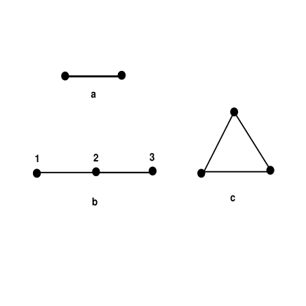
Figure 1: The simplest symmetric graphs. The graph in (b) is only symmetric with respect to the interchange of the vertices 1 and 3. The EoF in graph (a) is unbounded, that of graph (c) is bounded but much higher than that of vertices 1 and 3 in graph (b).

The potential for this graph is $V=\frac{1}{2}(x_{1}^{2}+x_{2}^{2}+\omega^{2}(x_{1}-x_{2})^{2})$. It represents the harmonic interaction of two atoms with frequency $\omega$ each trapped inside a harmonic well of unit frequency. The potential matrix is

$$\hat{V}=\left(\begin{array}[]{cc}1+\omega^{2}&-\omega^{2}\\ -\omega^{2}&1+\omega^{2}\end{array}\right),$$ (27)

with eigenvalues and eigenvectors

$$\omega_{1}^{2} := 1,\hskip 28.45274pt\ \ \ \ \ \ \ \ |e_{1}\rangle=\frac{1}{\sqrt{2}}\left(\begin{array}[]{c}1\\ 1\end{array}\right),$$ (30)

$$\omega_{2}^{2} := 1+2\omega^{2},\hskip 28.45274pt|e_{2}\rangle=\frac{1}{\sqrt{2}}\left(\begin{array}[]{c}1\\ -1\end{array}\right).$$ (33)

This leads to the following values for the relevant matrix elements:

$$({\Gamma_{x}})_{11} = \frac{1}{2}\left(\coth\frac{\beta}{2}+\frac{1}{\omega_{2}}\coth\frac{\beta\omega_{2}}{2}\right),\ \ \ \ ({\Gamma_{x}})_{12}=\frac{1}{2}\left(\coth\frac{\beta}{2}-\frac{1}{\omega_{2}}\coth\frac{\beta\omega_{2}}{2}\right),$$ (34)

$$({\Gamma_{p}})_{11} = \frac{1}{2}\left(\coth\frac{\beta}{2}+\omega_{2}\coth\frac{\beta\omega_{2}}{2}\right),\ \ \ \ ({\Gamma_{p}})_{12}=\frac{1}{2}\left(\coth\frac{\beta}{2}-\omega_{2}\coth\frac{\beta\omega_{2}}{2}\right).$$ (35)

Inserting these values in (24) we find the value of $\delta$,

$$\delta=\sqrt{\omega_{2}^{-1}{\coth\frac{\beta}{2}\coth\frac{\beta\omega_{2}}{2}}}$$ (36)

The equation $\delta=1$ determines the threshold temperature. Inserting this value of delta in (2) and (3) will determine the EoF as a function of the frequency $\omega$ and the temperature, shown in figure (2). The maximum entanglement obtains at zero temperature and is unbounded, it behaves as $E=-0.56+\log_{2}(w)+O(\omega^{-2})$ for large frequencies. The threshold temperature increases almost linearly with frequency.

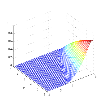
Figure 2: Thermal entanglement of the two modes (particles) (in units of ebits) associated to the graph in figure (1-a), as a function of temperature and frequency. $E$ is dimensionless and we are working in units in which $\omega$ and $T$ are also dimensionless.

4.2 The simplest three-vertex symmetric graphs

We now consider the graph shown in figure (1-b). This is one of the two symmetric graphs with three vertices. The other graph which is a triangle will be treated as a special case of $N$-vertices mean field clusters (for $N=3$). Note that this graph is symmetric only under the interchange of vertices $1$ and $3$. We will determine the EoF of these two modes. Our motivation for studying this graph is to show that entanglement can exist between next-nearest neighbors in open chains with an odd number of vertices, a property which we have seen also for higher than $3$ vertices in our calculations. Here the potential is

$$V=\frac{1}{2}(x_{1}^{2}+x_{2}^{2}+x_{3}^{2})+\frac{\omega^{2}}{2}((x_{1}-x_{2})^{2}+(x_{2}-x_{3})^{2}),$$ (37)

with the potential matrix

$$\hat{V}=\left(\begin{array}[]{ccc}1+\omega^{2}&-\omega^{2}&0\\ -\omega^{2}&1+2\omega^{2}&-\omega^{2}\\ 0&-\omega^{2}&1+\omega^{2}\end{array}\right).$$ (38)

The eigenvalues and eigenvectors are

$$\omega_{1}^{2} = 1,\hskip 28.45274pt\ \ \ \ \ \ \ \ |e_{1}\rangle=\frac{1}{\sqrt{3}}(1,1,1)^{T},$$ (39)

$$\omega_{2}^{2} = 1+\omega^{2},\hskip 28.45274pt\ |e_{2}\rangle=\frac{1}{\sqrt{2}}(1,0,-1)^{T},$$ (40)

$$\omega_{3}^{2} = 1+3\omega^{2},\hskip 28.45274pt|e_{3}\rangle=\frac{1}{\sqrt{6}}(1,-2,1)^{T}.$$ (41)

In this case we are only interested in the ground state entanglement. So only the matrix elements of $W$ and $W^{-1}$ need be calculated. One finds after straightforward calculations along the lines in the previous subsection the following value for $\delta$,

$$\delta=\sqrt{\frac{2+\sqrt{1+3\omega^{2}}}{3\sqrt{1+\omega^{2}}}}.$$ (42)

The value of this parameter is always less than $1$, and hence there is entanglement between the next-nearest neighbors at all frequencies. The interesting point is however that this entanglement is bounded. It obtains at very large frequencies where $\delta\longrightarrow 3^{-\frac{1}{4}}$, leading to $E_{inf}=13.62$ in units of $10^{-2}$ ebits.

4.3 Mean field clusters

Consider a mean field cluster of $N$ vertices in which every vertex is connected to $N-1$ other vertices. The potential matrix for this graph is given by

$$\hat{V}=(1+N\omega^{2})I-\omega^{2}\hat{E},$$ (43)

where $E$ is the matrix all of whose entries are equal to 1, $E_{ij}=1\ \ \ \forall\ \ \ i,\ \$ and $\ j$. Using the property $E^{2}=NE$, we find

$$W = \sqrt{1+N\omega^{2}}I+\frac{1-\sqrt{1+N\omega^{2}}}{N}E$$ (44)

$$W^{-1} = \frac{1}{\sqrt{1+N\omega^{2}}}(I+\frac{\sqrt{1+N\omega^{2}}-1}{N}E).$$ (45)

Using these matrices and equation (25) one finds the value of $\delta$ at zero temperature

$$\delta_{N}=\sqrt{\frac{2+(N-2)\sqrt{1+N\omega^{2}}}{N\sqrt{1+N\omega^{2}}}}$$ (46)

Inserting this into equations (2) and (3) gives the entanglement as a function of $N$ and frequency.
Let us first consider the special case of $3$ vertices, whose graph is a triangle, shown in figure (1-c) and compare it with result for the three-vertex graph shown in figure ( 1-b).
For $N=3$, we have $\delta_{3}=\sqrt{\frac{2+\sqrt{1+3\omega^{2}}}{3\sqrt{1+3\omega^{2}}}}$. The Eof saturates at $E_{inf}=40.08$ (in units of $10^{-2}$ ebits) for infinite frequencies.
Returning to (46) we can find the EoF in mean field clusters as a function of frequency for fixed number of vertices. The maximum EoF always occurs for infinitely large frequencies where $\delta$ tends to $\sqrt{\frac{N-2}{N}}$. Figure (3 ) shows the EoF as a function of $w$ for some mean field clusters with $N=4,6,8,12$ and $20$ vertices. These are the number of vertices of regular polyhedra, namely tetrahedron, octahedron, cube, dodecahedron and isocahedron respectively, which will be treated in the nest subsection.

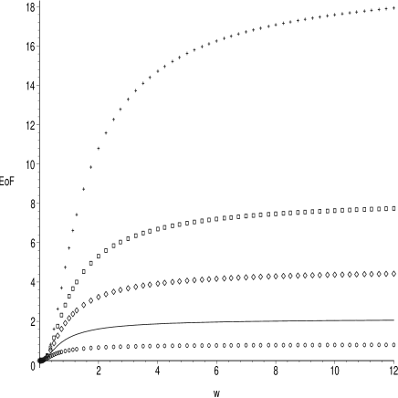
Figure 3: The EoF (in units of $10^{-2}$ ebits) of two vertices for mean field graphs with number of vertices from top to bottom $N=4,6,8,12$ and $20$.

Finally figure(4) shows how the maximum EoF decreases with increasing the number of vertices in mean field clusters. For large values of $N$ the EoF vanishes as $E\approx\frac{1.72\log N}{2N^{2}}$.

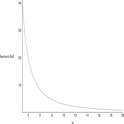
Figure 4: The maximum EoF (in units of $10^{-2}$ ebits) for mean field clusters as a function of the number of vertices.

4.4 Regular Polyhedra

In this section we consider the regular polyhedra, the tetrahedron ($N=4$), the cube ($N=8$), the octahedron ($N=6$), the dodecahedron ($N=20$) and the isocahedron ($N=12$). The tetrahedron is a mean field cluster with $N=4$, so we can use the results of the mean field cluster for this graph. For the other cases we follow the same procedure as above, i.e. determine the adjacency matrix which in turn determines the potential matrix from (26). The square root $W$ and the inverse square root $W^{-1}$ of $\hat{V}$ are calculated by diagonalization of $\hat{V}$. We can then calculate the necessary elements of $W$ and $W^{-1}$ in order to determine the EoF of pair of vertices in terms of the strength of the interaction $\omega$. It turns out that the $EoF$ is always an increasing function of $\omega$ and saturates for infinite frequencies. The maximum EoF attains its value for the nearest neighbors. Depending on the polyhedron, the EoF may or may not exist between next nearest neighbors. Furthermore compared with mean field clusters the EoF is always higher than that of mean field clusters, the difference is larger for higher frequencies. Figure (5) shows the EoF of the regular polyhedra in terms of the strength of interaction. Figure (6) compares the EoF of the octahedron with that of a mean field cluster with $6$ vertices. Finally table (1) compares the maximum EoF obtained in regular polyhedra with those of the mean field clusters of the same size (the same number of vertices) and the bounds found in [1].

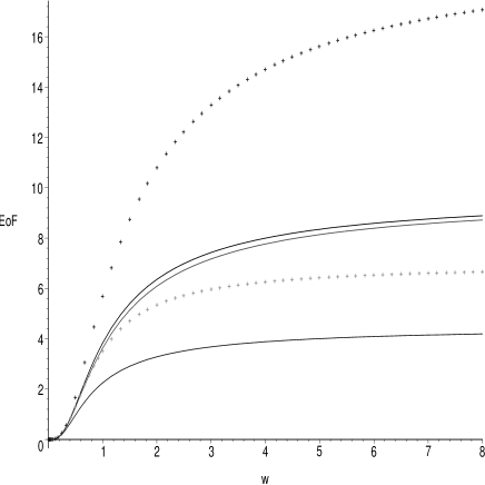
Figure 5: The EoF of adjacent vertices (in units $10^{-2}$ ebits) in regular polyhedra. The curves correspond from top to bottom to Tetrahedron, Cube, Octahedron, Dodecahedron and Isocahedron.

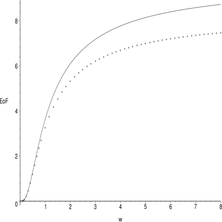
Figure 6: The EoF of adjacent vertices (in units $10^{-2}$ ebits) as a function of $w$ for the regular octahedron (line) and a six-vertex mean field cluster (dots).

Polyhedron	N	Mean field Cluster	$E_{{\rm inf}}$	$E_{max}$
Tetrahedron	4	19.74	19.74	19.74
Cube	8	8.30	9.80	19.74
Octahedron	6	4.68	9.74	10.75
Dodecahedron	20	2.15	7.00	11.12
Isocahedron	12	0.83	4.51	5.37

Table 1-The maximum entanglement ($E_{inf}$) in regular polyhedra and mean field graphs of the same size, compared with the bounds found in [1]. $N$ is the number of vertices of the polyhedron and the mean field graph.

Polyhedron	$E^{1}_{{\rm inf}}$	$E^{2}_{{\rm inf}}$	$E^{3}_{\rm{inf}}$	$E^{4}_{\rm{inf}}$	$E^{5}_{\rm{inf}}$
Tetrahedron	19.74	-	-	-	-
Cube	9.80	1.08	0.24	-	-
Octahedron	9.74	2.58	-	-	-
Dodecahedron	7.00	0	0	0	0
Isocahedron	4.51	0	0	0	0

Table 2-The EoF between different vertices in regular polyhedra. The superscript indicates the minimum distance between the vertices in terms of the number of edges. The $-$ sign indicates that such distances do not occur in the corresponding regular polyhedron.

4.5 Rings and rectangular lattices

For the $d$-dimensional cubic lattice, of $N^{d}$ vertices, the potential matrix is

$$\hat{V}=(1+2d\omega^{2})I-\omega^{2}\sum_{k=1}^{d}(\hat{T_{k}}+\hat{T_{k}}^{-1}),$$ (47)

where $T_{k}$ is the cyclic unit shift operator in the $k-$ direction. The eigenvalues and eigenvectors are as follows:

$$\omega_{s}^{2}={1+4\omega^{2}\sum_{k=1}^{d}\sin^{2}\frac{\pi s_{k}}{N}},\hskip 28.45274ptu_{\bf s}({\bf n}):=\frac{1}{\sqrt{N^{d}}}e^{\frac{2\pi i{\bf s\cdot n}}{N}}.$$ (48)

From these values one can easily obtain the relevant matrix elements of $W$ and $W^{-1}$. For example for the one dimensional lattice we will have

$${W^{\pm 1}}_{k,l}=\sum_{s=0}^{N-1}({1+4\omega^{2}\sin^{2}\frac{\pi s}{N}})^{\frac{\pm 1}{2}}e^{\frac{2\pi is(k-l)}{N}}.$$ (49)

As always the EoF increases with the strength of interaction. It turns out that EoF exists only between nearest neighbor sites. Figure (7) compares the EoF of rings with two very different size as a function of frequency. The interesting point is that, the difference for the number of vertices only shows itself when the frequency is high enough.
Figure (8) compares the EoF of $d-$ dimensional lattices for $d=1,2,3$ when $N\longrightarrow\infty$. For the infinite lattices, the sums in (49) turn into integrals and we will have for two adjacent vertices say $1$ and $2$ of one dimensional lattice,

$$W^{\pm 1}_{11} = \frac{1}{\pi}\int_{0}^{\pi}dx({1+4\omega^{2}\sin^{2}x})^{\pm\frac{1}{2}}$$ (50)

$$W^{\pm 1}_{12} = \frac{1}{\pi}\int_{0}^{\pi}dx({1+4\omega^{2}\sin^{2}x})^{\pm\frac{1}{2}}\cos{2x},$$ (51)

and for the two dimensional lattice

$$W^{\pm 1}_{11} = \frac{1}{\pi^{2}}\int_{0}^{\pi}dx\int_{0}^{\pi}dy[{1+4\omega^{2}(\sin^{2}x+\sin^{2}y})]^{\pm\frac{1}{2}}$$ (52)

$$W^{\pm 1}_{12} = \frac{1}{\pi^{2}}\int_{0}^{\pi}dx\int_{0}^{\pi}dy[{1+4\omega^{2}(\sin^{2}x+\sin^{2}y})]^{\pm\frac{1}{2}}\cos{2x}.$$ (53)

Table (3) compares the saturation values of EoF achieved in these cases with the maximum achievable EoF’s derived in [1].

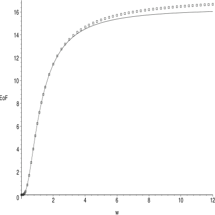
Figure 7: The EoF of two adjacent sites for rings with different number of vertices almost coincide for low frequencies, $N=11$ (points) $N=201$ (line).

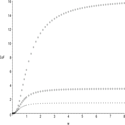
Figure 8: The EoF for infinite dimensional lattices as a function of frequency, from top to bottom $d=1,d=2$ and $d=3$.

d	$E_{{\rm inf}}$	$E_{{\rm max}}$
1	16.34	30
2	3.54	6.31
3	1.50	2.62

Table 3-The maximum EoF between adjacent vertices in d-dimensional rectangular lattices compared with the bounds found in [1].

5 Discussion

We have investigated the entanglement properties of the ground state of a quadratic Hamiltonian governing the harmonic interaction of bosonic modes or particles located on the vertices of symmetric graphs i.e. 1,2, and 3 dimensional rectangular lattices, mean field clusters and platonic solids. The entanglement has been calculated as a function of the interaction strength. In each case the EoF is an increasing function of the interaction strength and it saturates to a finite value dictated by the type of the graph. Our results confirm those of [1] in that the maximum values that we obtain are always less than the bounds found in that paper which correspond to a particular quadratic hamiltonian proved to allow for maximum achievable EoF between any two modes in the class of all quadratic hamiltonians. Some peripheral results may be interesting. First, in some symmetric graphs ( the cube, the octahedron and open chains with an odd number of vertices) there are entanglement between non-adjacent vertices, a property which is extraordinary for entanglement, since for rings it has been shown [12] that entanglement can not extend beyond the nearest neighbors. Second, in the case of two atoms vibrating in a molecule or ions vibrating in an ion trap, corresponding to the simple graph (1-a) the threshold temperature above which entanglement is destroyed, has been determined.

6 Acknowledgement

We would like to thank A. Bayat, I. Marvian, D. Lashkari, N. Majd, L. Memarzadeh, and A. Sheikhan for valuable discussions.

7 References

References

- [1] M. M. Wolf, E. Verstaete and J. I. Cirac, Phys. Rev. Lett. 92, 087903 (2004).
- [2] M. C. Arnesen, S. Bose, and V. Vedral, Phys. Rev. Lett. 87, 277901 (2001).
- [3] X. Wang, and P. Zanardi, Phys. Lett. A 301 (1-2),1 (2002).
- [4] A. Osterloh, L. Amico, G. Falci, and R. Fazio, Nature 416, 608 (2002).
- [5] M. K. O’Connor and W. K. Wootters, Phys. Rev. A 63, 052302 (2001).
- [6] B. Q. Jin, V. E. Korepin, Phys. Rev. A, 69, 120406 (2004).
- [7] T. Osborne, M. Nielsen, Entanglement in a simple quantum phase transition, quant-ph/0202162.
- [8] M. Asoudeh, and V. Karimipour, Phys. Rev. A 70, 052307 (2004).
- [9] B. Julsgaard, A. Kozhekin, and E. S. Polzik, Nature, 413, 400 (2000).
- [10] L. M. Duan, G. Giedke, J. I. Cirac, and P. Zoller, Phys. Rev. Lett. 84, 2722 (2000); R. Simon, Phys. Rev. Lett. 84, 2726 (2000).
- [11] R. F. Werner and M. M. Wolf, Phys. Rev. Lett. 86, 3658 (2001).
- [12] K. Audenaert, J. Eisert, M. B. Plenio, and R. F. Werner, Phys. Rev. A 66, 042327 (2002).
- [13] M. B. Plenio, J. Hartley, and J. Eisert, New J. Phys. 6, 36 (2004).
- [14] M. M. Wolf, G. Giedke, O. Krger, R. F. Werner, and J. I. Cirac, Phys. Rev. A 69, 052320 (2004).
- [15] G. Giedke, M. M. Wolf, O. Kr ger, R. F. Werner, and J. I. Cirac, Phys. Rev. Lett. 91, 107901 (2003).
- [16] M.M. Wolf, J. Eisert, M.B. Plenio, Phys. Rev. Lett. 90, 047904 (2003)
- [17] M. C. de Oliveira, Phys. Rev. A 70, 034303 (2004).
- [18] A. Serafini, F. Illuminati, and S. De Siena, J. Phys. B 37, L21 (2004).
- [19] S. J. van Enk, Phys. Rev. A 67, 022303 (2003).
- [20] J. R. Gittings and A. J. Fisher, Phys. Rev. A 66, 032305 (2002).
- [21] P. Giorda and P. Zanardi, quant-ph/0311058.
- [22] V. Vedral, Central Eur. J. Phys. 1, 289 (2003).
- [23] , A. Holevo, Probabilistic and statistical aspects of quantum theory (North-Holland, Publishing Company, 1982).
- [24] B. Englert and K. Wodkiewicz, Int. Jour. Quant. Information, vol 1, No. 2, (2003) 153-188.