Measuring the quality factor of a microwave cavity using superconduting qubit devices

Abstract

We propose a method to create superpositions of two macroscopic quantum states of a single-mode microwave cavity field interacting with a superconducting charge qubit. The decoherence of such superpositions can be determined by measuring either the Wigner function of the cavity field or the charge qubit states. Then the quality factor $Q$ of the cavity can be inferred from the decoherence of the superposed states. The proposed method is experimentally realizable within current technology even when the $Q$ value is relatively low, and the interaction between the qubit and the cavity field is weak.

I Introduction

Superconducting (SC) Josephson junctions are considered promising qubits for quantum information processing. This “artificial atom”, with well-defined discrete energy levels, provides a platform to test fundamental quantum effects, e.g., cavity quantum electrodynamics (QED). The study of the cavity QED of a SC qubit, e.g., in Ref. you , can also open new directions for studying the interaction between light and solid state quantum devices. These can result in novel controllable electro-optical quantum devices in the microwave regime, such as microwave single-photon generators and detectors. Cavity QED can allow the transfer of information among SC qubits via photons, used as information bus.

Recently, different information buses using bosonic systems, which play a role analogous to a single-mode light field, have been proposed to mediate the interaction between the SC qubits. These bosonic “information bus” systems can be modelled by: nanomechanical resonators (e.g., in Refs. nano ); large junctions (e.g., Ref. wang ); current-biased large junctions (e.g., Refs. large ), and LC oscillators (e.g., Refs. lc ). However, the enormous versatility provided by photons should stimulate physicists to pay more attention to SC qubits interacting via photons,while embedded inside a QED cavity.

Several theoretical proposals have analyzed the interaction between SC qubits and quantized  saidi ; you ; you1 ; liu ; gao ; vourdas ; zagoskin or classical fields zhou ; paspalakis ; liu1 . The strong coupling of a single photon to a SC charge qubit has been experimentally demonstrated wallraff by using a one-dimensional transmission line resonator blais . But, the QED effect of the SC qubit inside higher-dimensional cavities has not been experimentally observed. The main roadblocks seem to be: i) whether the cavity quality factor $Q$ can still be maintained high enough when the SC qubit is placed inside the cavity. Different from atoms, the effect of the SC qubit on the $Q$ value of the cavity is not negligible due to its complex structure and larger size. ii) The higher-dimensional QED cavity has relatively large mode volume, making the interaction between the cavity field and the qubit not be strong enough for the required quantum operations within the decoherence time. iii) The transfer of information among different SC qubits requires the qubit-photon interaction to be switched on/off by the external classical flux on time scales of the inverse Josephson energy. A higher cavity $Q$ value, a stronger qubit-photon interaction, and a faster switching interaction for the SC qubit QED experiments, seem difficult to achieve anytime soon.

In view of the above problems, it would be desirable to explore the possibility to demonstrate a variety of relatively simple cavity QED phenomena with a SC qubit. The determination of the cavity $Q$ value is a very important first step for the experiments on cavity QED with SC qubits. However, theoretical calculations of the $Q$ value are not always easy to perform because of the complexity of the circuit. Recent experiments pkd on broadband SC detectors showed that the $Q$ value of the SC device can reach $2\times 10^{6}$, which indicates that relatively simple experiments using cavity QED with a SC qubit are possible.

In this paper, we propose an experimentally feasible method which can be used to demonstrate a simple cavity QED effect of the SC qubit. For instance, superpositions of two macroscopic quantum states of a single-mode microwave cavity field can be created by the interaction between a SC charge qubit and the cavity field. At this stage, the injected light field is initially a coherent state, which can be easily prepared. The decoherence of the created superposition states can be further determined by measuring either the Wigner function of the cavity field or the charge qubit states. Then the cavity $Q$ value can be inferred from this decoherence measurement. Our proposal only needs few operations with a relatively low Q value. Also, we do not need to assume a very fast sweep rate of the external magnetic field for switching on/off the qubit-field interaction. Furthermore, the qubit-field interaction is not necessarily resonant.

We begin in Sec. II with a brief overview of the qubit-field interaction. In Sec. III, we discuss how to prepare superpositions of two different cavity field states under the condition of large detuning. In Sec. IV, the cavity $Q$ value is determined by the tomographic reconstruction of the cavity field Wigner function. In Sec. V, we show an alternative method to determine the $Q$ value according to the states of the qubit. Finally, we list our conclusions.

II Theoretical model

We briefly review a model of a SC charge qubit inside a cavity. The Hamiltonian can be written as you ; you1 ; liu ; gao

$$H=\hbar\omega a^{\dagger}a+E_{z}\sigma_{z}$$ (1)

$$-\,E_{J}\sigma_{x}\cos\left[\frac{\pi}{\Phi_{0}}\left(\Phi_{c}I+\eta\,a+\eta^{*}\,a^{\dagger}\right)\right],$$

where the first two terms respectively represent the free Hamiltonians of the cavity field with frequency $\omega$ for the photon creation (annihilation) operator $a^{\dagger}\,(a)$, and the qubit charging energy

$$E_{z}=-2E_{\rm ch}(1-2n_{g})\,,$$ (2)

which depends on the gate charge $n_{g}$. The single-electron charging energy is $E_{\rm ch}=e^{2}/2(C_{g}+2C_{J})$ with the capacitors $C_{g}$ and $C_{J}$ of the gate and the Josephson junction, respectively. The dimensionless gate charge, $n_{g}=C_{g}V_{g}/2e$, is controlled by the gate voltage $V_{g}$. Here, $\sigma_{z}$, $\sigma_{x}$ are the Pauli operators, and the charge excited state $|e\rangle$ and ground state $|g\rangle$ correspond to the eigenstates $|\!\downarrow\rangle=\left(\begin{array}[]{l}0\\ 1\end{array}\right)$ and $|\!\uparrow\rangle=\left(\begin{array}[]{l}1\\ 0\end{array}\right)$ of the spin operator $\sigma_{z}$, respectively. $I$ is an identity operator. The third term is the nonlinear qubit-photon interaction. $E_{J}$ is the Josephson energy for a single junction. The parameter $\eta$ is defined as $\eta=\int_{S}\mathbf{u}(\mathbf{r})\cdot d\mathbf{s}$ with the mode function of the cavity field $\mathbf{u}(\mathbf{r})$, $S$ is the surface defined by the contour of the SQUID. We can decompose the cosine in Eq. (1) into classical and quantized parts. The quantized parts $\sin[\pi(\eta\,a+H.c.)/\Phi_{0}]$ and $\cos[\pi(\eta\,a+H.c.)/\Phi_{0}]$ can be further expanded as a power series in $a\,(a^{\dagger})$. To estimate the qubit-photon coupling constant, the qubit is assumed to be inside a full-wave cavity with the standing-wave form for a single-mode magnetic field scully

$$B_{x}=-i\sqrt{\frac{\hbar\omega}{\varepsilon_{0}Vc^{2}}}(a-a^{\dagger})\cos(kz).$$ (3)

The polarization of the magnetic field is along the normal direction of the surface area of the SQUID, located at an antinode of the standing-wave mode. The mode function $\sqrt{\hbar\omega/\varepsilon_{0}Vc^{2}}\cos(kz)$ can be assumed to be independent of the integral area because the maximum linear dimension of the SQUID, e.g., even for $50\,\,\mu$m, is much less than $0.1$ cm, the shortest microwave wavelength of the cavity field. Then, in the microwave regime, the estimated range of values for $\pi\eta/\Phi_{0}$ is: $8.55\times 10^{-6}\leq\pi\eta/\Phi_{0}\leq 1.9\times 10^{-3}$, for a fixed area of the SQUID, e.g., $50\,\mu$m $\times 50\,\mu$m. If the light field is not so strong (e.g., the average number of photons inside the cavity $N=\langle a^{\dagger}a\rangle\leq 100$), then we can only keep the first order of $\pi\eta/\Phi_{0}$ and safely neglect all higher orders. Thus, the Hamiltonian (1) becomes

$$H=\hbar\omega a^{\dagger}a+E_{z}\sigma_{z}-\,E_{J}\sigma_{x}\cos(\frac{\pi\Phi_{c}}{\Phi_{0}})$$

$$+\frac{\pi E_{J}}{\Phi_{0}}\sin(\frac{\pi\Phi_{c}}{\Phi_{0}})\left(\eta\,a\,\sigma_{+}+\eta^{*}\,a^{\dagger}\,\sigma_{-}\right).$$ (4)

It is clear that the qubit-photon interaction can be controlled by the classical flux $\Phi_{c}$, after neglecting higher-orders in $\pi\eta/\Phi_{0}$.

III Preparation of macroscopic superposition states

The qubit-photon system can be initialized by adjusting the gate voltage $V_{g}$ and the external flux $\Phi_{c}$ such that $n_{g}=1/2$ and $\Phi_{c}=0$, then the dynamics of the qubit-field is governed by the Hamiltonian

$$H_{1}=\hbar\omega a^{\dagger}a-E_{J}\sigma_{x}.$$ (5)

Now there is no interaction between the cavity field and the qubit; thus, the cavity field and the qubit evolve according to Eq. (5). We assume that the qubit-photon system works at low temperatures $T$ ( e.g., $T=30$ mK in Ref. nakamura ), then the mean number of thermal photons $\langle n_{th}\rangle$ in the cavity can be negligible in the microwave regime liu , and the cavity is approximately considered in the zero temperature environment. The initial state of the cavity field is prepared by injecting a single-mode coherent light

$$|\alpha\rangle=\exp\left\{-\frac{|\alpha|^{2}}{2}\right\}\sum_{n=0}\frac{\alpha^{n}}{\sqrt{n!}}|n\rangle\,,$$ (6)

into the cavity. Here, without loss of generality, $\alpha$ is assumed to be a real number, and $a|\alpha\rangle=\alpha|\alpha\rangle$. The qubit is assumed to be initially in the ground state $|g\rangle$. After a time interval $\tau_{1}=\hbar\pi/4E_{J}$, the qubit ground state $|g\rangle$ is transformed as $|g\rangle\rightarrow\left(|g\rangle+i|e\rangle\right)/\sqrt{2}$; then, the qubit-photon state evolves into

$$|\psi(\tau_{1})\rangle=\frac{1}{\sqrt{2}}(|g\rangle+i|e\rangle)|\alpha\rangle\,.$$ (7)

Here we have neglected the free evolution phase factor $e^{-i\omega\tau_{1}}$ in $\alpha$.

Now, we assume that the gate voltage and the magnetic flux are switched to $n_{g}\neq 1/2$ (this value of $n_{g}$ will be specified later) and $\Phi_{c}=\Phi_{0}/2$, respectively. Then the qubit-photon interaction appears and the effective Hamiltonian governing the dynamic evolution of the qubit-photon can be written as (see Appendix A)

$$H_{2}=\hbar\omega_{-}a^{\dagger}a+\frac{1}{2}\hbar\Omega\sigma_{z}+\hbar\frac{|g|^{2}}{\Delta}\left(1+2a^{{\dagger}}a\right)|e\rangle\langle e|\,,$$ (8)

with $\omega_{-}=\omega-|g|^{2}/\Delta$ and $g=(\pi\eta E_{J})/(\hbar{\Phi_{0}})$. The detuning $\Delta=\Omega-\omega>0$ between the qubit transition frequency $\Omega=-4E_{ch}(1-2n_{g})/\hbar$ and the cavity field frequency $\omega$ is assumed to satisfy the large detuning condition

$$\frac{\pi E_{J}|\eta|}{\hbar\Phi_{0}\Delta}\ll 1.$$ (9)

The unitary evolution operator corresponding to Eq. (8) can be written as

$$U(t) = \exp\left[-i\left(\omega_{-}a^{\dagger}a+\frac{\Omega}{2}\sigma_{z}\right)t\right]$$ (10)

$$\times \exp\left[-itF(a^{\dagger}a)|e\rangle\langle e|\right],$$

here, the operator $F(a^{\dagger}a)$ is expressed as

$$F(a^{\dagger}a)=\frac{|g|^{2}}{\Delta}(1+2a^{\dagger}a).$$ (11)

With an evolution time $\tau_{2}$, the state (7) evolves into

$$|\psi(\tau_{2})\rangle=\frac{1}{\sqrt{2}}\left[|g\rangle|\beta\rangle+i\exp(i\theta)|e\rangle|\beta^{\prime}\rangle\right]$$ (12)

where a global phase $\exp(-i\Omega\tau_{2}/2)$ has been neglected, $\theta=(\Omega-|g|^{2}/\Delta)\tau_{2}$, $\beta=\alpha\exp[-i\omega_{-}\tau_{2}]$, and $\beta^{\prime}=\beta\exp(-i\phi)$, with $\phi=2|g|^{2}\tau_{2}/\Delta$. Equation (12) shows that a phase shift $\phi$ is generated for the coherent state $|\beta\rangle$ of the cavity field when the qubit is in the excited state $|e\rangle$, but the qubit ground state $|g\rangle$ does not induce an extra phase for the coherent state $|\beta\rangle$.

The gate voltage and the magnetic field are now adjusted such that the conditions $n_{g}=1/2$ and $\Phi_{c}=0$ are satisfied; then the qubit-photon interaction is switched off. Now let the system evolve a time $\tau^{\prime}=\tau_{1}=\hbar\pi/4E_{J}$, then Eq. (12) becomes

$$|\psi(\tau_{2})\rangle = \frac{1}{2}|g\rangle\otimes[|\beta\rangle-\exp(i\theta)|\beta^{\prime}\rangle]$$ (13)

$$+ i\frac{1}{2}|e\rangle\otimes[|\beta\rangle+\exp(i\theta)|\beta^{\prime}\rangle],$$

where a free phase factor $e^{-i\omega\tau_{1}}$ in the cavity field states $|\beta\rangle$ and $|\beta e^{-i\phi}\rangle$ has been neglected.

The superpositions of two distinguished coherent states can be conditionally generated by measuring the charge states of the qubit as,

$$|\beta_{\pm}\rangle=N^{-1}_{\pm}[|\beta\rangle\pm\exp(i\theta)|\beta^{\prime}\rangle],$$ (14)

where the $+$ ($-$) correspond to the measurement results $|e\rangle$ ($|g\rangle$), and the normalized constants $N_{\pm}$ are determined by

$$N^{2}_{\pm}=2\pm 2\cos\theta^{\prime}\exp\!\left[-2|\alpha|^{2}\sin^{2}\left(\frac{\phi}{2}\right)\right],$$ (15)

where $\theta^{\prime}=|\alpha|^{2}\sin\phi-\theta$, and the relation $|\beta|^{2}=|\alpha|^{2}$ is used.

Due to $\Phi_{c}=0$, after the superpositions in Eq.(14) are created, the dynamic evolution of the cavity field is only affected by its dissipation, characterized by the decay rate $\gamma$, which can be expressed by virtue of the cavity quality factor $Q$ as $Q=\omega/\gamma$. Now let the cavity field described by the states $|\beta_{+}\rangle$ or $|\beta_{-}\rangle$ evolve a time $\tau_{3}$; then the reduced density matrices of the superpositions can be described by

$$\rho_{\pm}(\tau_{3})=\frac{1}{N^{2}_{\pm}}\left\{|\beta u\rangle\langle\beta u|+|\beta^{\prime}u\rangle\langle\beta^{\prime}u|\right.$$

$$\left.\pm C|\beta^{\prime}u\rangle\langle\beta u|\pm C^{*}|\beta u\rangle\langle\beta^{\prime}u|\right\},$$ (16)

where

$$C=\exp(i\theta)\exp\left\{|\alpha|^{2}(1-e^{-i\phi})(u^{2}-1)\right\}$$ (17)

and

$$u\equiv u(\tau_{3})=\exp\left(-\frac{\gamma}{2}\tau_{3}\right)=\exp\left(-\,\frac{\omega\tau_{3}}{2Q}\right).$$ (18)

It is clearly shown that the mixed state in Eq. (III) is strongly affected by the $Q$ value. Equation (III) is derived for zero temperature since thermal photons are negligible at low-temperature. Equations (III-18) show that the information of the cavity quality factor $Q$ can be encoded in a reduced density matrix of the cavity field. The $Q$ value can be determined using two different methods, after encoding its information in Eqs.(III-18). Below, we will discuss these two approaches.

IV Measuring $Q$ by photon state tomography

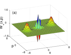
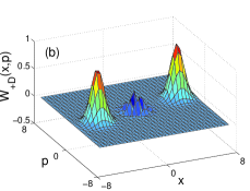
Figure 1: (Color online) Wigner functions $W_{+}(x,p)$ of Eq. (14) and $W_{+D}(x,p)$ of Eq. (III) for the cavity field without and with the energy dissipation are shown in (a) and (b), for the input state $|\alpha\rangle$ with $\overline{n}=16$. Here the Wigner functions $W_{+}(x,p)$ and $W_{+D}(x,p)$ are normalized to $\pi N_{+}$.

The state $\rho$ of the optical field is generally visualized when it is represented by a Wigner function hans in the position $x$ and momentum $p$ space, which is written as

$$W(x,p)=\frac{1}{\pi}\int_{-\infty}^{\infty}\langle x-x^{\prime}|\rho|x+x^{\prime}\rangle e^{i2px^{\prime}}{\rm d}x^{\prime}.$$ (19)

The Wigner function $W(x,p)$ can be experimentally measured by state tomographic techniques hans . For any two coherent states, $|\alpha\rangle$ and $|\beta\rangle$, the Wigner function $W(x,p)$ can be represented as

$$W_{\alpha,\beta}(x,p) = \frac{1}{\pi}\int_{-\infty}^{\infty}\langle x-x^{\prime}|\alpha\rangle\langle\beta|x+x^{\prime}\rangle e^{i2px^{\prime}}{\rm d}x^{\prime}$$ (20)

$$= \frac{1}{\pi}\exp\left\{-\frac{1}{2}(|\alpha|^{2}+|\beta|^{2}-2\alpha\beta^{*})\right\}$$

$$\times \exp\left\{-(x-q_{1})^{2}-(p+iq_{2})^{2}\right\}$$

with $q_{1}=(\alpha+\beta^{*})/\sqrt{2}$ and $q_{2}=(\alpha-\beta^{*})/\sqrt{2}$. The Wigner functions $W_{\pm}(x,p)$ and $W_{\pm D}(x,p)$ for the states (14) and (III) were calculated (see Appendix B) by using Eq. (20). Comparing the tomographically measured results for the states (14) and (III), the $Q$ factor of the cavity can be finally determined, as explained below by using an example.

We further numerically calculate the Wigner functions $W_{\pm}(x,p)$ and $W_{\pm D}(x,p)$ of the states (14) and (III) from the SC qubit parameters and given operation durations. Using current values for experimental data, the basic physical parameters can be specified as follows. We assume that the SC Cooper-pair box is made from aluminum, with a BCS energy gap of $\sim 2.4$K (about 50 GHz) lehnert , the charge energy $E_{\rm ch}$ and the Josephson energy $E_{\rm J}$ are $4E_{\rm ch}/h=149$ GHz and $2E_{\rm J}/h=13.0$ GHz, respectively lehnert . The frequency of the cavity field is taken as $40$ GHz, corresponding to a wavelength $\sim 0.75$ cm. The above numbers show that the SC energy gap is the largest energy, so the quasi-particle excitation on the island can be well suppressed at low temperatures, e.g., $20$ mK . The SQUID area is assumed to be about $50\,\mu$m $\times 50\,\mu$m, then the absolute value $|g|$ of the qubit-photon coupling constant is about $|g|=4\times 10^{6}$ rad s^-1.

Let us now prepare entangled qubit-photon states as in Eq. (13). Any gate charge value $n_{g}$ in Eq. (2), in which the large detuning condition in Eq. (9) is satisfied, can be chosen to realize our proposal. For concreteness, we give an example. The gate voltage is adjusted such that the gate charge is $n_{g}\approx 0.634233$, which can be experimentally achieved lehnert , then the detuning $\Delta=\Omega-\omega\approx 9.0\times 10^{6}$ rad s^-1. Thus, $\Omega$ is about $40$ GHz plus $1.4$ MHz, and $|g|^{2}/\Delta\,\simeq\,0.27$ MHz. We can also find that $\Delta/|g|\approx 2.3$, so a large-detuning condition can be used xm ; pt . For a given Josephson energy, $2E_{J}/h=13.0$ GHz, the operation times $\tau_{1}=4.8\times 10^{-12}$ s, required to prepare a superposition of $|e\rangle$ and $|g\rangle$ with equal probabilities, is much less than the qubit relaxation time $T_{1}=1.3\,\mu$s and dephasing time $T_{2}=5$ ns. We can choose the duration $\tau_{2}$ for a given input coherent state $|\alpha\rangle$ with the condition, that the distance $|\beta-\beta^{\prime}|$ between two coherent states $|\beta\rangle$ and $|\beta^{\prime}\rangle$ satisfies

$$|\beta-\beta^{\prime}|=2|\alpha|\sin\left(\frac{\phi}{2}\right)>1.$$ (21)

So the lower bound of the duration $\tau_{2}$ can be given as

$$\tau_{2}=\frac{\Delta}{|g|^{2}}\arcsin\left(\frac{1}{2|\alpha|}\right)\,,$$ (22)

when $0\leq\phi\leq\pi$. Equation (22) shows that a shorter $\tau_{2}$ can be obtained for a higher intensity $|\alpha|$ with fixed detuning $\Delta$ and coupling constant $g$.

As an example, we plot the Wigner function of the superposition $|\beta_{+}\rangle$ in Fig. 1(a) for an input coherent light $|\alpha\rangle$ with the mean photon number $\overline{n}=|\alpha|^{2}=16$. We choose a simple case $\phi=\pi$, corresponding to the operation time $\tau_{2}\approx 0.93\,\mu$s, which is less than the qubit lifetime $T_{1}$ and the cavity field lifetime $T_{\rm ph}\approx 2\,\mu$s for a bad cavity with $Q=5\times 10^{5}$. In such a case, $\beta^{\prime}=-\beta$ and the phase $\theta$ is about $0.996\,[{\rm mod}\,2\pi]$ rad. Other parameters used in Fig. 1 are given above. If we set the evolution time $\tau_{3}=0.1\,\mu$s, then the Wigner function of Eq. (III) for the above cavity quality factor is shown in Fig. 1(b). The central structure in Fig. 1(a) represents the coherence of the quantum state. In Fig. 1(b), we find that the height of the Wigner function $W_{+D}(x,p)$, especially for the central structure, is reduced by the environment. Comparing Fig. 1(a) and Fig. 1(b), it is found that the coherence of the superposed states is suppressed by the environment, and the decoherence of superpositions is tied to the energy dissipation of the cavity field. Then, the $Q$ value can in principle be estimated by measuring the Wigner functions of Eqs. (III) and (14), and comparing these two kinds of results.

V Determining $Q$ by readout of charge states

The determination of the $Q$ value by measuring the Wigner function needs optical instruments. In solid state experiments, the charge states are typically measured. Instead of using optical instruments, it would be desirable to obtain the $Q$ value by measuring charge states. This will be our goal here. The process to achieve this can be described as follows.

i) According to the measurements on the charge qubit states in Eq.(13), the qubit-photon states are projected to $|g\rangle\otimes|\beta_{-}\rangle$ or $|e\rangle\otimes|\beta_{+}\rangle$, respectively. After the evolution time $\tau^{\prime}_{3}$, a $\pi/2$ quantum operation is performed on the qubit with the duration $T=\hbar\pi/4E_{J}$. Then, the qubit ground state $|g\rangle$, or excited state $|e\rangle$, is transformed into the superposition $(|g\rangle+i|e\rangle)/\sqrt{2}$, or $(i|g\rangle+|e\rangle)/\sqrt{2}$, and the photon states $|\beta_{\pm}\rangle$ evolve into mixed states after the evolution time $\tau=\tau^{\prime}_{3}+T$, and the photon-qubit states can be expressed as

$$\rho_{Q+F}=\frac{1}{2}(|g\rangle\pm i|e\rangle)(\langle g|\mp i\langle e|)\otimes\rho_{\pm}(\tau)\,,$$ (23)

with subscripts $Q$ and $F$ denoting the qubit and cavity field, respectively. The reduced density matrices $\rho_{\pm}(\tau)$ take the same form as in Eq. (III) with $\tau$ replacing $\tau_{3}$.

ii) After the above procedure, the qubit-photon interaction is switched on by applying the external magnetic flux $\Phi_{e}=\Phi_{0}/2$. By using Eq. (10), Eq. (23) evolves into

$$2\rho_{A+F}^{(1)} = |g\rangle\langle g|\otimes U_{1}(\tau_{4})\rho_{\pm}(\tau)U^{\dagger}_{1}(\tau_{4})$$

$$+ |e\rangle\langle e|\otimes U_{2}(\tau_{4})\rho_{\pm}(\tau)U^{\dagger}_{2}(\tau_{4})$$

$$\mp i\exp(-i\Omega_{-}\tau_{4})|g\rangle\langle e|\otimes U_{1}(\tau_{4})\rho_{\pm}(\tau)U^{\dagger}_{2}(\tau_{4})$$

$$\pm i\exp(+i\Omega_{-}\tau_{4})|e\rangle\langle g|\otimes U_{2}(\tau_{4})\rho_{\pm}(\tau)U^{\dagger}_{1}(\tau_{4})$$

with $\Omega_{-}=\Omega-|g|^{2}/\Delta$, and a shorter evolution time $\tau_{4}$. For example, $\tau_{4}$ is less than the lifetime $T_{1}$ of the qubit at least. The time evolution operators $U_{1}(\tau_{4})$ and $U_{2}(\tau_{4})$ in Eq. (V) are

$$U_{1}(\tau_{4}) = \exp\left[-i\omega_{-}\,a^{\dagger}a\,\tau_{4}\right],$$ (25a)

$$U_{2}(\tau_{4}) = \exp\left[-i\omega_{+}\,a^{\dagger}a\,\tau_{4}\right].$$ (25b)

with $\omega_{\pm}=\omega\pm|g|^{2}/\Delta$. After this qubit-photon interaction, the information of the $Q$ value is encoded.

iii) The qubit-photon coupling is switched off and a $\pi/2$ rotation is made on the qubit. If the state of the cavity field is prepared to $|\beta_{-}\rangle$ of Eq. (14) in the first step, then the qubit is in the ground state $|g\rangle$. After measuring the qubit states, the photon states are projected to

$$\rho_{e/g}=\frac{1}{4}(A\pm B)$$ (26a)

where the sign $$``+" |e\rangle ``-" |g\rangle A B$$ corresponds to the excited state measurement, but corresponds to the ground state measurement. The operators and are

$$A = \sum_{i=1}^{2}U_{i}(\tau_{4})\rho_{-}(\tau)U^{\dagger}_{i}(\tau_{4}),$$ (26b)

$$B = 2\,{\rm Re}[\exp(-i\Omega_{-}\tau_{4})U_{1}(\tau_{4})\rho_{-}(\tau)U^{\dagger}_{2}(\tau_{4})].$$ (26c)

After tracing out the cavity field state, the probabilities corresponding to measuring charge states $|e\rangle$ and $|g\rangle$ are

$$P_{e/g}(\tau) = {\rm Tr}_{F}\,\left(\rho_{e/g}\right)$$ (27)

$$= \frac{1}{2}\left\{1\pm{\rm Re}({\rm Tr}_{F}[\exp(-i\varphi)\rho_{-}(\tau)])\right\}$$

with $\varphi=(\Omega_{-}-2|g|^{2}a^{\dagger}a/\Delta)\tau_{4}$. Then the measurement probabilities are related to the $Q$ values. Substituting $\rho_{-}(\tau)$ into Eq.(27), we can obtain

$${\rm Re}\left\{{\rm Tr}[\exp(-i\varphi)\rho_{-}(\tau)]\right\}$$ (28a)

$$=\frac{2}{N^{2}_{-}}\exp\left[-2\alpha(\tau)\sin^{2}\phi^{\prime}\right]\cos\left[\Omega_{-}\tau_{4}-\alpha(\tau)\sin(2\phi^{\prime})\right]$$

$$-\frac{1}{N^{2}_{-}}\cos\left[\theta_{-}-|\alpha|^{2}\sin\phi+\theta-\Omega_{-}\tau_{4}\right]\exp\left(+G_{-}-\Gamma\right)$$

$$-\frac{1}{N^{2}_{-}}\cos\left[\theta_{+}+|\alpha|^{2}\sin\phi-\theta-\Omega_{-}\tau_{4}\right]\exp\left(-G_{+}-\Gamma\right)$$

with the parameters

$$\phi^{\prime} = \frac{|g|^{2}}{\Delta}\tau_{4},$$ (28b)

$$\Gamma = 2|\alpha|^{2}\sin^{2}(\frac{\phi}{2}),$$ (28c)

$$\alpha(\tau) = |\alpha u(\tau)|^{2},$$ (28d)

$$G_{\pm} = 2\alpha(\tau)\sin\phi^{\prime}\sin(\phi\pm\phi^{\prime}),$$ (28e)

$$\theta_{\pm} = 2\alpha(\tau)\cos(\phi\pm\phi^{\prime})\sin\phi^{\prime}.$$ (28f)

From Eq. (28), we find that $\phi^{\prime}$ should satisfy the condition $\phi^{\prime}\neq n\pi$ for $\phi=\pi$, in order to describe the dissipation effect; here $n$ is an integer. Generally speaking, if one of the functions $G_{+}$, $G_{-}$, $\theta_{+}$, $\theta_{-}$, $\sin\phi^{\prime}$, or $\sin(2\phi^{\prime})$ is nonzero, then this is enough to encode the $Q$ value, which can be obtained from Eq. (28), together with Eq. (18), using $\tau$ instead of $\tau_{3}$.

However, if the superposition of the cavity fields is prepared to the state $|\beta_{+}\rangle$ in the first step, then the ground and excited state measurements make the cavity field collapse to state

$$\rho^{\prime}_{g/e}=\frac{1}{4}(A^{\prime}\pm B^{\prime}),$$ (29)

where $A^{\prime}$ and $B^{\prime}$ have the same forms as Eqs. (26b) and (26c), just with the replacement of $\rho_{-}(\tau)$ by $\rho_{+}(\tau)$.

The probabilities $P^{\prime}_{g}(\tau)$ and $P^{\prime}_{e}(\tau)$ to measure the qubit states $|g\rangle$ and $|e\rangle$ corresponding to the prepared state $|\beta_{+}\rangle$ of Eq. (14) after a dissipation interval $\tau$, can also be obtained as

$$P_{g/e}^{\prime}(\tau)=\frac{1}{2}\left\{1\pm{\rm Re}({\rm Tr}_{F}[\exp(-i\varphi)\rho_{+}(\tau)])\right\}$$ (30)

where ${\rm Re}\{{\rm Tr}_{F}[\exp(-i\varphi)\rho_{+}(\tau)]\}$ can be obtained by replacing $N_{-}$ with $N_{+}$, and replacing the sign $``-"$ before the second and third terms with the sign $``+"$ in Eq. (28a)

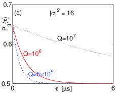
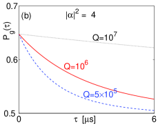
Figure 2: (Color online) The probability $P_{g}(\tau)$ to measure the qubit ground state $|g\rangle$ as a function of the evolution time $\tau$. This $P_{g}(\tau)$ is shown for several values of the quality factor $Q$ and for different intensities of the input coherent state $|\alpha\rangle$.

To determine the Q values by probing the charge states, the measurement should be made for two times, the first measurement is for the preparation of the superpositions of the cavity field. After the first measurement, we make a suitable qubit rotation, and then make the qubit interact with the cavity field for a duration $\tau_{4}$. Finally, the second measurement is made and the $Q$ information is encoded in the measured probabilities. The different evolution times $\tau$ correspond to the different measuring probabilities for given $\tau_{4}$ and other parameters $|\alpha|$, $\Delta$, and so on. For example, the probabilities $P_{e/g}(\tau)$ for several special cases are discussed as follows when the prepared state is $|\beta_{-}\rangle$. If we assume that the qubit rotations and qubit-photon dispersive interaction are made without energy dissipation of the cavity field, e.g., $\tau=0$, then the measuring probabilities $P_{e/g}(\tau=0)$ only encode the information of the cavity field but do not include the quality factor $Q$. If the coherence of the states $|\beta_{\pm}\rangle$ nearly disappears after time $\tau$, then the state $|\beta_{-}\rangle$ becomes a classical statistical mixture

$$\rho_{-}(\tau)=\frac{1}{N^{2}_{-}}\left[|\beta u(\tau)\rangle\langle\beta u(\tau)|+|\beta^{\prime}u(\tau)\rangle\langle\beta^{\prime}u(\tau)|\right].$$ (31)

The probabilities $P_{e/g}(\tau)$ are then reduced to

$$P_{e/g}(\tau) = \frac{1}{N^{2}_{-}}\pm\frac{\exp\left[-2\alpha(\tau)\sin^{2}\phi^{\prime}\right]}{N^{2}_{-}}$$

$$\times \cos\left[\Omega_{-}\tau_{4}-\alpha(\tau)\sin(2\phi^{\prime})\right],$$

which tends to $1/2$ for $|\alpha|^{2}\gg 1$. If $\tau>1/\gamma=t_{\rm ph}$ of the single-photon state lifetime, then the photons of the states $|\beta_{\pm}\rangle$ are completely dissipated into the environment. In this case, the cavity quality factor $Q$ cannot be encoded in the probabilities $P_{e/g}(\tau)$ even with some qubit and qubit-photon states operations.

As an example, let us consider how $P_{g}(\tau)$ varies with the evolution time $\tau$ with the cavity field dissipation. We assume that the evolution time $\tau_{4}=(\pi/2)(\Delta/|g|^{2})$, that is, $\phi^{\prime}=\pi/2$. Then, the $\tau$-dependent probabilities $P_{g}(\tau)$ for the initially prepared state $|\beta_{-}\rangle$ are given in Fig. 2(a) with the same parameters as in Fig. 1, except with different cavity quality factors $Q$. In order to see how the probability $P_{g}(\tau)$ changes with the intensity $|\alpha|^{2}$ of the input coherent state $|\alpha\rangle$, we plot $P_{g}(\tau)$ in Fig. 2(b) with the same parameters as Fig. 2(a) except changing the intensity to $|\alpha|^{2}=4$ from $|\alpha|^{2}=16$. Figure 2 shows that both the higher quality factor $Q$ and weaker intensity $|\alpha|^{2}$ of the input cavity field correspond to a larger probability $P_{g}$ of the ground state for the fixed evolution time $\tau$. For fixed $Q$ and $\tau$, the weaker intensity $|\alpha|^{2}$ corresponds to a higher measuring probability. We plot $P_{g}(\tau)$ in Fig. 2 considering the simple case $\phi=\pi$. However, if we consider another $\phi$, then $|\alpha|^{2}$ should be chosen such that it satisfies the condition $2|\alpha|\sin(\phi/2)>1$. In conclusion, the quality factor $Q$ can be determined from the probabilities $P_{e/g}(\tau)$ of measuring the qubit states with a finite cavity field evolution time $\tau$.

VI Discussions and conclusions

We discussed how to measure the cavity quality factor $Q$ by using the interaction between a single-mode microwave cavity field and a controllable superconducting charge qubit. Two methods are proposed. One measures the Wigner function of the state (III) by using a standard optical method hans . Another approach measures the qubit states. Using this last method, the information of the $Q$ value can be encoded into the reduced density matrix of the cavity field, and at the same time the qubit makes a $\pi/2$ rotation. Thus, with a suitable qubit-photon interaction time, information on the $Q$ value is then transferred to the qubit-photon states. Finally, after another $\pi/2$ rotation, the charge qubit states are measured, and the $Q$ value can be obtained, as shown in Fig. 2, Eqs. (28) and Eq. (18). However, it should be noticed that it is easy to measure charge states than to measure photon states in superconducting circuits.

Our proposal shows that a cavity QED experiment with a SC qubit can be performed even for a relatively low $Q$ values, e.g., $Q\sim 10^{6}$. Initially, a coherent state is injected into the cavity, which is relatively easy to do experimentally. Although all rotations of the qubit are chosen as $\pi/2$ to demonstrate our proposal, other rotations can also be used to achieve our goal.

To simplify these studies and without loss of generality, we have assumed two components $|\beta\rangle$ and $|\beta\exp(i\phi)\rangle$ for superpositions with $\phi=\pi$ phase difference in our numerical demonstrations. Of course, other superpositions can also be used to realize our purpose. The only condition to satisfy is that the distance between the two states $|\beta\rangle$ and $|\beta\exp(i\phi)\rangle$ should be larger than one. In order to obtain a numerical estimate for the detuning, we specify a value of the gate charge number $n_{g}$. However, any gate charge that satisfies the large-detuning condition can be chosen to realize our proposal.

Although we did not give a detailed description of another resonance-based approach, it should be pointed out that the $Q$ values can also be determined by virtue of the resonant qubit-photon interaction. For example, if the superpositions liu of the vacuum and the single photon state are experimentally prepared, then we can follow the same steps as in Sec. III and IV to obtain the $Q$ value. This method rinner has been applied to micromasers, where the qubits are two-level atoms. However, the coherent states and non-resonant qubit-photon interaction should be easier to do experimentally than the approach using single-photon states and resonant qubit-photon interaction.

Our proposal can also be generalized to the models used in Refs. wallraff ; blais , which are experimentally accessible. We hope that our proposal can open new doors to experimentally test the $Q$ value and motivate further experiments on cavity quantum electrodynamics with SC qubits.

VII acknowledgments

This work was supported in part by the National Security Agency (NSA) and Advanced Research and Development Activity (ARDA) under Air Force Office of Research (AFOSR) contract number F49620-02-1-0334, and by the National Science Foundation grant No. EIA-0130383.

Appendix A Effective hamiltonian with larger detuning

The Hamiltonian $H=H_{0}+H_{1}$ of the two-level atom interacting with a single-mode cavity field can be written as

$$H_{0} = \frac{1}{2}\hbar\Omega\sigma_{z}+\hbar\omega a^{\dagger}a,$$ (33a)

$$H_{1} = \hbar(ga^{\dagger}\sigma_{-}+g^{*}a\sigma_{+})$$ (33b)

with a complex number $g$. Let us assume $\Delta=\Omega-\omega>0$ and $g/\Delta\ll 1$. The eigenstates and corresponding eigenvalues of the free Hamiltonian $H_{0}$ are

$$|e\rangle\otimes|n\rangle \Longrightarrow n\hbar\omega+\frac{1}{2}\hbar\Omega,$$ (34a)

$$|g\rangle\otimes|m\rangle \Longrightarrow m\hbar\omega-\frac{1}{2}\hbar\Omega$$ (34b)

In the interaction picture, any state can be written as

$$|\psi(t)\rangle=U(t,t_{0})|\psi(t_{0})\rangle$$ (35)

with

$$U(t,t_{0}) = 1+\frac{1}{i\hbar}\int_{t_{0}}^{t}H_{\rm int}(t_{1}){\rm d}t_{1}$$

$$+ \left(\frac{1}{i\hbar}\right)^{2}\int_{t_{0}}^{t}\int_{t_{0}}^{t_{1}}H_{\rm int}(t_{1})H_{\rm int}(t_{2}){\rm d}t_{1}{\rm d}t_{2}+\cdots$$

here $H_{\rm int}=U^{\dagger}_{0}(t)H_{1}U_{0}(t)$ with $U_{0}(t)=\exp\{-iH_{0}t/\hbar\}$. In the basis $\{|E_{l}\rangle\}=\{|e\rangle\otimes|n\rangle,\,\,|g\rangle\otimes|m\rangle\}$, Eq. (A) can be expressed as

$$U(t,t_{0}) = 1+$$

$$+ \frac{1}{i\hbar}\int_{t_{0}}^{t}\sum_{l,m}|E_{l}\rangle\langle E_{l}|H_{\rm int}(t_{1})|E_{m}\rangle\langle E_{m}|{\rm d}t_{1}+\cdots.$$

After neglecting the fast-oscillating factor and keeping the first order term in $g/\Delta$, $U(t,t_{0})$

$$U(t,t_{0})=U(t,0)=U(t)$$ (37)

$$\approx 1-i\frac{|g|^{2}}{\Delta}\int_{0}^{t}{\rm d}t_{1}[(n+1)|e,n\rangle\langle e,n|-n|g,n\rangle\langle g,n|],$$

where we assume $t_{0}=0$. Finally, we obtain the effective Hamiltonian in the interaction picture as

$$H_{\rm eff}=\hbar\frac{|g|^{2}}{\Delta}(|e\rangle\langle e|aa^{\dagger}-|g\rangle\langle g|a^{\dagger}a).$$ (38)

Returning Eq. (38) to the Schrödinger picture, Eq. (10) is obtained. This method can be generalized to obtain the effective Hamiltonian of the model with many two-level system interacting with a common single-mode field. Equation (10) can also be obtained by using the Fröhlich-Nakajima transformation Fro ; Nakajima ; wu ; sun .

Appendix B Wigner functions of superposition and mixed states

For completeness, we explicitly write the Wigner functions $W_{\pm}(x,p)$ of the superposition states in Eq. (14) as follows:

$$W_{\pm}(x,p)$$

$$=\frac{1}{\pi N^{2}_{\pm}}\left\{\exp\left[-\left(x-\sqrt{2}\,{\rm Re}\beta\right)^{2}-\left(p-\sqrt{2}\,{\rm Im}\beta\right)^{2}\right]\right.$$

$$+\exp\left[-\left(x-\sqrt{2}\,{\rm Re}\beta^{\prime}\right)^{2}-\left(p-\sqrt{2}\,{\rm Im}\beta^{\prime}\right)^{2}\right]$$

$$\left.\pm 2{\rm Re}\left[P\exp\left(-\left(x-\wp_{1}\right)^{2}-\left(p+i\wp_{2}\right)^{2}\right)\right]\right\}\,,$$ (39)

with

$$P = \exp(-i\theta)\exp[-|\alpha|^{2}(1-e^{i\phi})],$$ (40)

$$\wp_{1} = \frac{1}{\sqrt{2}}(\beta+\beta^{\prime*}),$$ (41)

$$\wp_{2} = \frac{1}{\sqrt{2}}(\beta-\beta^{\prime*}).$$ (42)

The Wigner functions $W_{\pm D}(x,p)$ of the mixed states in Eq. (III) with dissipation can be written as

$$W_{\pm D}(x,p)$$

$$=\frac{1}{\pi N^{2}_{\pm}}\left\{\exp\left[-\left(x-u\sqrt{2}\,{\rm Re}\beta\right)^{2}-\left(p-u\sqrt{2}\,{\rm Im}\beta\right)^{2}\right]\right.$$

$$+\exp\left[-\left(x-u\sqrt{2}\,{\rm Re}\beta^{\prime}\right)^{2}-\left(p-u\sqrt{2}\,{\rm Im}\beta^{\prime}\right)^{2}\right]$$

$$\left.\pm 2{\rm Re}\left[P\exp\left(-\left(x-u\,\wp_{1}\right)^{2}-\left(p+iu\,\wp_{2}\right)^{2}\right)\right]\right\}.$$ (43)

References

- (1) J.Q. You and F. Nori, Phys. Rev. B 68, 064509 (2003); Physica E 18, 33 (2003).
- (2) A.D. Armour, M.P. Blencowe, and K.C. Schwab, Phys. Rev. Lett. 88, 148301 (2002); E.K. Irish and K. Schwab, Phys. Rev. B 68, 155311 (2003); A.N. Cleland and M.R. Geller, Phys. Rev. Lett. 93, 070501 (2004); I. Martin, A. Shnirman, L. Tian, and P. Zoller, Phys. Rev. B 69, 125339 (2004); L. Tian, quant-ph/0412185.
- (3) Y.D. Wang, P. Zhang, D.L. Zhou, and C.P. Sun, Phys. Rev. B 70, 224515 (2004).
- (4) L.F. Wei, Yu-xi Liu, and F. Nori, Europhys. Lett. 67, 1004 (2004); Phys. Rev. B 71, 134506 (2005); A. Blais, A.M. van den Brink, and A.M. Zagoskin, Phys. Rev. Lett. 90, 127901 (2003); I. Chiorescu, P. Bertet, K. Semba, Y. Nakamura, C.J.P.M. Harmans, and J.E. Mooij, Nature 431, 159 (2004).
- (5) A. Shnirman, G. Schön, and Z. Hermon, Phys. Rev. Lett. 79, 2371 (1997); F. Plastina and G. Falci, Phys. Rev. B 67, 224514 (2003).
- (6) W. A. Al-Saidi and D. Stroud, Phys. Rev. B 65, 224512 (2002).
- (7) J.Q. You, J.S. Tsai, and F. Nori, Phys. Rev. B 68, 024510 (2003); Physica E 18, 35 (2003).
- (8) Yu-xi Liu, L.F.Wei, and F. Nori, Erophys. Lett. 67, 941 (2004).
- (9) Y.B. Gao, Y.D. Wang, and C. P. Sun, Phys. Rev. A 71, 032302 (2005); P. Zhang, Z. D. Wang, J. D. Sun, C. P. Sun, quant-ph/0407069, Phys. Rev. A (in press).
- (10) C.P. Yang, S.I. Chu, and S. Han, Phys. Rev. A 67, 042311 (2003)
- (11) A.M. Zagoskin, M. Grajcar, and A.N. Omelyanchouk, Phys. Rev. A 70, 060301(R) (2004)
- (12) Z.Y. Zhou, S.I. Chu, and S. Han, Phys. Rev. B 66, 054527 (2002).
- (13) E. Paspalakis and N.J. Kylstra, J. Mod. Opt. 51, 1679 (2004).
- (14) Yu-xi Liu, J.Q. You, L.F. Wei, C.P. Sun, and F. Nori, quant-ph/0501047.
- (15) A. Wallraff, D.I. Schuster, A. Blais, L. Frunzio, R.S. Huang, J. Majer, S, Kumar, S.M. Girvin, and R.J. Schoelkopf, Nature 431, 162 (2004).
- (16) A. Blais, R.S. Huang, A. Wallraff, S.M. Girvin, and R.J. Schoelkopf, Phys. Rev. A 69, 062320 (2004).
- (17) P.K. Day, H.G. LeDuc, B. A. Mazin, A. Vayonakis, and J. Zmuidzinas, Nature 425, 817 (2003).
- (18) M.O. Scully and M.S. Zubairy Quantum optics (Cambridge University Press, Cambridge, 1997).
- (19) Y. Nakamura, Y.A. Pashkin, and J.S. Tsai, Nature 398, 786 (1999); Phys. Rev. Lett. 87, 246601 (2001); Y. Nakamura, Y.A. Pashkin, T. Yamamoto and J.S. Tsai ibid. 88, 047901 (2002); Y.A. Pashkin, T. Yamamoto, O. Astafiev, Y. Nakamura, D.V. Averin, and J.S. Tsai, Nature 421, 823 (2003); T. Yamamoto, Y.A. Pashkin, O. Astafiev, Y. Nakamura, and J.S. Tsai, ibid. 425, 941 (2003).
- (20) K.W. Lehnert, K. Bladh, L.F. Spietz, D. Gunnarsson, D.I. Schuster, P. Delsing, and R.J. Schoelkopf, Phys. Rev. Lett. 90, 027002 (2003).
- (21) M. Brune, E. Hagley, J. Dreyer, X. Maître, A. Maali, C. Wunderlich, J.M. Raimond, and S. Haroche, Phys. Rev. Lett. 77, 4887 (1996); X. Maître, E. Hagley, G. Nogues, C. Wunderlich, P. Goy, M. Brune, J.M. Raimond, and S. Haroche, Phys. Rev. Lett. 79, 769 (1997).
- (22) D. Vitali, P. Tombesi, and G.J. Milburn, Phys. Rev. Lett. 79, 2442 (1997).
- (23) H. Uwazumi, T. Shimatsu, and Y. Kuboki, J. of Appl. Phys. 91, 7095 (2002).
- (24) S. Rinner, H. Walther, and E. Werner, Phys. Rev. Lett. 93, 160407 (2004).
- (25) H. Fröhlich, Phys. Rev. 79, 845 (1950).
- (26) S. Nakajima, Adv. Phys. 4, 463 (1953).
- (27) Y. Wu, Phys. Rev. A 54, 1586 (1996).
- (28) C.P. Sun, Yu-xi Liu, L. F. Wei, and F. Nori, quant-ph/0506011.
- (29) Hans-A. Bachor, A Guide to Experiments in Quantum Optics (Wiley-VCH, New York, 1998)