Quantum damped oscillator I:
dissipation and resonances

Abstract

Quantization of a damped harmonic oscillator leads to so called Bateman’s dual system. The corresponding Bateman’s Hamiltonian, being a self-adjoint operator, displays the discrete family of complex eigenvalues. We show that they correspond to the poles of energy eigenvectors and the corresponding resolvent operator when continued to the complex energy plane. Therefore, the corresponding generalized eigenvectors may be interpreted as resonant states which are responsible for the irreversible quantum dynamics of a damped harmonic oscillator.

1 Introduction

The damped harmonic oscillator is one of the simplest quantum systems displaying the dissipation of energy. Moreover, it is of great physical importance and has found many applications especially in quantum optics. For example it plays a central role in the quantum theory of lasers and masers [1, 2, 3].

As is well known there is no room for the dissipative phenomena in the standard Hilbert space formulation of Quantum Mechanics. The Schrödinger equation defines one-parameter unitary group and hence the quantum dynamics is perfectly time-reversible. The usual approach to include dissipation is the quantum theory of open systems [4, 5, 6, 7]. In this approach the dynamics of a quantum system is no longer unitary but it is defined by a semigroup of completely positive maps in the space of density operators [8] (for recent reviews see e.g. [9, 10]).

There is, however, another way to describe dissipative quantum systems based on the old idea of Bateman [11]. Bateman has shown that to apply the standard canonical formalism of classical mechanics to dissipative and non-Hamiltonian systems, one can double the numbers of degrees of freedom, so as to deal with an effective isolated classical Hamiltonian system. The new degrees of freedom may be assumed to represent a reservoir. Applying this idea to damped harmonic oscillator one obtains a pair of damped oscillators (so called Bateman’s dual system): a primary one and its time reversed image. The Bateman dual Hamiltonian has been rediscovered by Morse and Feshbach [12] and Bopp [13] and the detailed quantum mechanical analysis was performed by Feshbach and Tikochinski [14]. The quantum Bateman system was then analyzed by many authors (see the detailed historical review [15] with almost 600 references!).

Surprisingly, this system is still worth to study and it shows its new interesting features. Recently it was analyzed in [16] in connection with quantum field theory and quantum groups (see also [17, 18]). Different approach based on the Chern-Simons theory was applied in [19]. In a recent paper [20] a damped oscillator was quantized by using Feynman path integral formulation (see also [21]). Moreover, the corresponding geometric phase was calculated and found to be directly related to the ground-state energy of the standard one-dimensional linear harmonic oscillator. Bateman’s system has been also studied as a toy model for the recent proposal by ’t Hooft about deterministic quantum mechanics [22, 23].

In the present paper we propose a slightly different approach to the Bateman system. The unusual feature of the Bateman Hamiltonian is that being a self-adjoint operator it displays a family of complex eigenvalues. We show that these eigenvalues correspond to the poles of energy eigenvectors and the corresponding resolvent operator when continued to the complex energy plane. The similar analysis for the toy model of a quantum damped system was performed in [24, 25]. Eigenvectors corresponding to the poles of the resolvent are well known in the scattering theory as resonant states [29, 30]. It shows that the appearance of resonances is responsible for the dissipation in the Bateman system. Obviously, the time evolution is perfectly reversible when considered on the corresponding system Hilbert space ${\cal H}=L^{2}(\mathbb{R}^{2})$. It is given by the 1-parameter group of unitary transformations $U(t)=e^{-i\widehat{H}t}$. It turns out that there are two natural subspaces ${\cal S}_{\pm}\in{\cal H}$ such that $U(t)$ restricted to ${\cal S}_{\pm}$ defines only two semigroups: $U(t\geq 0)$ on ${\cal S}_{-}$, and $U(t\leq 0)$ on ${\cal S}_{+}$. These two semigroups are related by the time reversal operator $\cal T$ (see Section 6).

Our analysis is based on a new representation of the Bateman Hamiltonian, cf. Section 4. This representation is directly related to the old observation of Pontriagin [31] (see Section 3 for review) that any non-Hamiltonian system of the form

$$\dot{x}_{k}=X_{k}(x_{1},\ldots,x_{N})\ ,\ \ \ \ k=1,2,\ldots,N\ ,$$ (1.1)

may be treated as a Hamiltonian one in the extended phase-space $(x_{1},\ldots,x_{N},p_{1},\ldots,p_{N})$ with the Hamiltonian

$$H(x_{1},\ldots,x_{N},p_{1},\ldots,p_{N})=\sum_{k=1}^{N}p_{k}\,X_{k}(x_{1},\ldots,x_{N})\ .$$ (1.2)

Note, that the above Hamiltonian has exactly the form considered by ’t Hooft [22].

From the mathematical point of view the natural language to analyze the Bateman system is the so called rigged Hilbert space approach to quantum mechanics [26, 27, 28]. There are two natural rigged Hilbert spaces, or Gel’fand triplets, corresponding to subspaces ${\cal S}_{\pm}$. We shall comment on that in Section 8.

2 Bateman Hamiltonian

The classical equation of motion for one-dimensional damped oscillator with unit mass reads

$$\ddot{x}+2\gamma\dot{x}+\kappa x\;=\;0\ ,$$ (2.1)

where $\gamma>0$ denotes the damping constant. Introducing Bateman’s dual system

$$\ddot{y}-2\gamma\dot{y}+\kappa y\;=\;0\ ,$$ (2.2)

one may derive booth equations from the following Lagrangian

$$L(x,\dot{x},y,\dot{y})=\dot{x}\dot{y}-\kappa xy+\gamma(x\dot{y}-\dot{x}y)\ .$$ (2.3)

Introducing canonical momenta

$$p_{x}=\dot{y}-\gamma y\,,\qquad p_{y}=\dot{x}+\gamma x\,,$$ (2.4)

one easily finds the corresponding Hamiltonian

$$H(x,y,p_{x},p_{y})=p_{x}p_{y}-\gamma(xp_{x}-yp_{y})+\omega^{2}xy\ ,$$ (2.5)

where

$$\omega=\sqrt{\kappa-\gamma^{2}}\ .$$ (2.6)

Throughout the paper we shall consider the underdamped case, i.e. $\kappa>\gamma^{2}$.

Now, assuming symmetric Weyl ordering the canonical quantization is straightforward and leads to the following self-adjoint operator in the Hilbert space $L^{2}(\mathbb{R}^{2},dxdy)$:

$$\hat{H}=\hat{H}_{0}+\hat{H}_{I}\ ,$$ (2.7)

where

$$\hat{H}_{0}=\hat{p}_{x}\hat{p}_{y}+\omega^{2}\hat{x}\hat{y}\ ,$$ (2.8)

and

$$\hat{H}_{I}=-\frac{\gamma}{2}\Big{(}(\hat{x}\hat{p}_{x}+\hat{p}_{x}\hat{x})-(\hat{y}\hat{p}_{y}+\hat{p}_{y}\hat{y})\Big{)}\ .$$ (2.9)

Note, that

$$[\hat{H}_{0},\hat{H}_{I}]=0\ .$$ (2.10)

Following Feshbach and Tichochinsky [14] one introduces annihilation and creation operators

$$\hat{A} = \frac{1}{2\sqrt{\hbar\omega}}\Big{[}(\hat{p}_{x}+\hat{p}_{y})-i\omega(\hat{x}+\hat{y})\Big{]}\,,$$ (2.11)

$$\hat{B} = \frac{1}{2\sqrt{\hbar\omega}}\Big{[}(\hat{p}_{x}-\hat{p}_{y})-i\omega(\hat{x}-\hat{y})\Big{]}\,.$$ (2.12)

They satisfy the standard CCRs

$$[\hat{A},\hat{A}^{\dagger}]=[\hat{B},\hat{B}^{\dagger}]=1\ ,$$ (2.13)

and all other commutators vanish. It turns out that the transformed Hamiltonian is given by (2.7) with

$$\hat{H}_{0}=\hbar\omega(\hat{A}^{\dagger}\hat{A}-\hat{B}^{\dagger}\hat{B})\ ,\qquad\hat{H}_{I}=i\hbar\gamma(\hat{A}^{\dagger}\hat{B}^{\dagger}-\hat{A}\hat{B})\ .$$ (2.14)

It is easy to see [14, 16] that the dynamical symmetry associated with the Bateman’s Hamiltonian is that of $SU(1,1)$. Indeed, constructing the following generators:

$$\hat{J}_{1} = \frac{1}{2}\,(\hat{A}^{\dagger}\hat{B}^{\dagger}+\hat{A}\hat{B})\,,$$ (2.15)

$$\hat{J}_{2} = \frac{i}{2}\,(\hat{A}^{\dagger}\hat{B}^{\dagger}-\hat{A}\hat{B})\,,$$ (2.16)

$$\hat{J}_{3} = \frac{1}{2}\,(\hat{A}^{\dagger}\hat{A}+\hat{B}\hat{B}^{\dagger})\,,$$ (2.17)

one easily shows that they satisfy $su(1,1)$ commutation relations:

$$[\hat{J}_{1},\hat{J}_{2}]=i\hat{J}_{3}\ ,\ \ \ \ \ \ [\hat{J}_{3},\hat{J}_{2}]=i\hat{J}_{1}\ ,\ \ \ \ \ \ [\hat{J}_{1},\hat{J}_{3}]=i\hat{J}_{2}\ .$$ (2.18)

Moreover, the following operator

$$\hat{J}_{0}=\frac{1}{2}\,(\hat{A}^{\dagger}\hat{A}-\hat{B}^{\dagger}\hat{B})\,,$$ (2.19)

defines the corresponding $su(1,1)$ Casimir operator. One easily shows that

$$\hat{J}^{2}_{0}=\frac{1}{4}+\hat{J}^{2}_{3}-\hat{J}^{2}_{1}-\hat{J}^{2}_{2}\ .$$ (2.20)

It is therefore clear that the Hamiltonian (2.14) can be rewritten in terms of $su(1,1)$ generators as

$$\hat{H}_{0}=2\hbar\omega\hat{J}_{0}\,,\qquad\hat{H}_{I}=2\hbar\gamma\hat{J}_{2}\,.$$ (2.21)

The algebraic structure arising in this approach enables one to solve the corresponding eigenvalue problem. Let us define two mode eigenvectors $|n_{A},n_{B}\rangle$:

$$\hat{A}^{\dagger}\hat{A}|n_{A},n_{B}\rangle=n_{A}|n_{A},n_{B}\rangle\ ,\hskip 28.45274pt\hat{B}^{\dagger}\hat{B}|n_{A},n_{B}\rangle=n_{B}|n_{A},n_{B}\rangle\ .$$ (2.22)

It is convenient to introduce

$$j=\frac{1}{2}(n_{A}-n_{B})\ ,\hskip 28.45274ptm=\frac{1}{2}(n_{A}+n_{B})\ ,$$ (2.23)

and to label the corresponding eigenvectors of $\hat{J}_{0}$ and $\hat{J}_{3}$ by $|j,m\rangle$ rather than $|n_{A},n_{B}\rangle$:

$$\hat{J}_{0}|j,m\rangle = j|j,m\rangle\ ,$$ (2.24)

$$\hat{J}_{3}|j,m\rangle = \left(m+\frac{1}{2}\right)|j,m\rangle\ .$$ (2.25)

Clearly,

$$j=0,\pm\frac{1}{2},\pm 1,\pm\frac{3}{2},\ldots,\hskip 28.45274ptm=|j|,|j|+1,|j|+2,\ldots\ .$$ (2.26)

Finally, defining

$$|\psi^{\pm}_{jm}\rangle=\exp\left(\mp\frac{\pi}{2}\hat{J}_{1}\right)|jm\rangle\ ,$$ (2.27)

one obtains

$$\hat{H}|\psi^{\pm}_{jm}\rangle=E^{\pm}_{jm}|\psi^{\pm}_{jm}\rangle\ ,$$ (2.28)

with

$$E^{\pm}_{jm}=2\hbar\omega j\pm i\hbar\gamma(2m+1)\ .$$ (2.29)

Let us emphasize that the eigenvectors corresponding to energies (2.29) cannot be normalized and should be considered as generalized eigenvectors not belonging to the Hilbert space of the problem.

3 Canonical quantization of non-Hamiltonian systems

As is well known any dynamical system may be regarded as a part of a larger Hamiltonian system. Bateman’s approach is based on adding to the primary system a time reversed (dual) copy. Together they define a Hamiltonian system. There exists, however, a general approach to canonical quantization of non-Hamiltonian systems based on an old observation of Pontriagin [31]. Suppose we are given an arbitrary non-Hamiltonian system described by

$$\dot{\bf x}={\bf X}({\bf x})\ ,$$ (3.1)

where $\bf X$ is a vector field on some configuration space $Q$. For simplicity assume that $Q\subset\mathbb{R}^{N}$, that is, the system has $N$ degrees of freedom. This system may be lifted to the Hamiltonian system on the phase space ${\cal P}=Q\times\mathbb{R}^{N}$ as follows: one defines the Hamiltonian $H:{\cal P}\longrightarrow\mathbb{R}$ by

$$H({\bf x},{\bf p})={\bf p}\cdot{\bf X}({\bf x})=\sum_{l=1}^{N}\,p_{l}X_{l}({\bf x})\ ,$$ (3.2)

where $({\bf x},{\bf p})=(x_{1},\ldots,x_{N},p_{1},\ldots,p_{N})$ denote canonical coordinates on $\cal P$. The corresponding Hamilton equations read as follows:

$$\dot{x}_{k} = \{x_{k},H\}=X_{k}(x)\ ,$$ (3.3)

$$\dot{p}_{k} = \{p_{k},H\}=-\sum_{l=1}^{N}p_{l}\frac{\partial X_{l}(x)}{\partial x_{k}}\ ,$$ (3.4)

for $k=1,\ldots,N$. In the above formulae $\{\ ,\ \}$ denotes the standard Poisson bracket on $\cal P$

$$\{F,G\}=\sum_{k=1}^{N}\left(\frac{\partial F}{\partial x_{k}}\frac{\partial G}{\partial p_{k}}-\frac{\partial G}{\partial x_{k}}\frac{\partial F}{\partial p_{k}}\right)\ .$$ (3.5)

Clearly, the formulae (3.3) reproduce our initial dynamical system (3.1) on $Q$. The canonical quantization is now straightforward. Assuming the symmetric Weyl ordering one obtains the following formula for the quantum Hamiltonian

$$\hat{H}_{\rm quantum}={\rm W}\left(\sum_{l=1}^{N}\,p_{l}X_{l}({\bf x})\right)\ ,$$ (3.6)

where ${\rm W}(f)$ denotes the Wigner-Weyl transform of a space-phase function $f=f({\bf x},{\bf p})$. Recall, that the Wigner-Weyl transform of $f$ is defined as follows

$$\hat{f}={\rm W}(f)=\int d\mbox{\boldmath$\sigma$}\int d\mbox{\boldmath$\tau$}\,\widetilde{f}(\mbox{\boldmath$\sigma$},\mbox{\boldmath$\tau$})\exp\left\{i\sum_{k=1}^{N}\left(\sigma_{k}\hat{x}_{k}+\tau_{k}\hat{p}_{k}\right)\right\}\ ,$$ (3.7)

where $\widetilde{f}(\mbox{\boldmath$\sigma$},\mbox{\boldmath$\tau$})$ denotes the Fourier transform of $f({\bf x},{\bf p})$. Clearly, $\hat{H}_{\rm quantum}$ defines a Schrödinger system in $L^{2}(\mathbb{R}^{N},d{\bf x})$.

Consider now a damped harmonic oscillator described by

$$\ddot{x}+2\gamma\dot{x}+\kappa x=0\ .$$

The above 2nd order equation may be rewritten as a dynamical system on $\mathbb{R}^{2}$

$$\dot{x}_{1} = -\gamma x_{1}+\omega x_{2}\ ,$$ (3.8)

$$\dot{x}_{2} = -\gamma x_{2}-\omega x_{1}\ ,$$ (3.9)

with $\omega$ defined in (2.6). Clearly this system is not Hamiltonian if $\gamma\neq 0$. However, applying the above Pontriagin procedure one arrives at the Hamiltonian system on $\mathbb{R}^{4}$ defined by the following damped harmonic oscillator Hamiltonian:

$$H({\bf x},{\bf p})=\omega(p_{1}x_{2}-p_{2}x_{1})-\gamma(p_{1}x_{1}+p_{2}x_{2})\ .$$ (3.10)

The corresponding Hamilton equations of motion read

$$\dot{\bf x}=\hat{F}{\bf x}\ ,\hskip 28.45274pt\dot{\bf p}=-\hat{F}^{\rm T}{\bf p}\ ,$$ (3.11)

where

$$\hat{F}=\left(\begin{array}[]{cc}-\gamma&\omega\\ -\omega&-\gamma\end{array}\right)\ ,$$ (3.12)

and $\hat{F}^{\rm T}$ denotes the transposition of $\hat{F}$. One may ask what is the relation between Bateman’s Hamiltonian (2.5) and that obtained via Pontriagin procedure (3.10). Surprisingly they are related by the following simple canonical transformation $(x,y,p_{x},p_{y})\longrightarrow(x_{1},x_{2},p_{1},p_{2})$:

$$x_{1} = \frac{p_{y}}{\sqrt{\omega}}\ ,\hskip 42.67912ptp_{1}\,=\,-\sqrt{\omega}\,y$$ (3.13)

$$x_{2} = -\sqrt{\omega}\,x\ ,\hskip 28.45274ptp_{2}\,=\,-\frac{p_{x}}{\sqrt{\omega}}\ .$$ (3.14)

Assuming the symmetric Weyl ordering one obtains the following representation of the quantum Bateman’s Hamiltonian (2.7) with

$$\hat{H}_{0}=\omega(\hat{p}_{1}\hat{x}_{2}-\hat{p}_{2}\hat{x}_{1})\ ,$$ (3.15)

and

$$\hat{H}_{I}=-\frac{\gamma}{2}(\hat{p}_{1}\hat{x}_{1}+\hat{x}_{1}\hat{p}_{1}+\hat{p}_{2}\hat{x}_{2}+\hat{x}_{2}\hat{p}_{2})\ .$$ (3.16)

4 Spectral properties of the Hamiltonian

4.1 Polar representation

The formula (3.10) for $H$ considerably simplifies in polar coordinates:

$$x_{1}+ix_{2}=re^{i\varphi}\ .$$

Defining the corresponding conjugate momenta

$$p_{\varphi}=L_{3}\ ,\hskip 28.45274ptp_{r}=\frac{{\bf x}{\bf p}}{r}\ ,$$ (4.1)

with $L_{3}$ denoting 3rd component of ${\bf L}={\bf x}\times{\bf p}$ in $\mathbb{R}^{3}$, one finds

$$H=-\omega p_{\varphi}-\gamma rp_{r}\ .$$ (4.2)

The Hamilton equations in polar representation have the following simple form:

$$\dot{\varphi}=-\omega\ ,\hskip 28.45274pt\dot{p}_{\varphi}=0\ ,$$ (4.3)

and

$$\dot{r}=-\gamma r\ ,\hskip 28.45274pt\dot{p}_{r}=\gamma p_{r}\ .$$ (4.4)

The polar representation nicely shows that the Hamiltonian dynamics consists in pure oscillation in $\varphi$–sector and dissipation (pumping) in $r$–sector ($p$–sector). In our opinion it is the most convenient representation to deal with .

The quantization of (4.2) leads to (2.7) with

$$\hat{H}_{0}=-\omega\hat{p}_{\varphi}=i\omega\hbar\,\frac{\partial}{\partial\varphi}\ ,$$ (4.5)

and

$$\hat{H}_{I}=i\gamma\hbar\left(r\frac{\partial}{\partial r}+1\right)=-\gamma\left(r\hat{p}_{r}-\frac{i\hbar}{2}\right)\ ,$$ (4.6)

where the radial momentum $\hat{p}_{r}$ is defined by

$$\hat{p}_{r}=-i\hbar\left(\frac{\partial}{\partial r}+\frac{1}{2r}\right)\ .$$ (4.7)

One easily finds the polar representation of the $su(1,1)$ generators:

$$\hat{J}_{1} = -\frac{\hbar}{4}\Big{(}\frac{\partial^{2}}{\partial r^{2}}+\frac{1}{r^{2}}\frac{\partial^{2}}{\partial\phi^{2}}\Big{)}-\frac{1}{4\hbar}r^{2}\,,$$ (4.8)

$$\hat{J}_{2} = \frac{i}{2}\Big{(}r\frac{\partial}{\partial r}+1\Big{)}\,,$$ (4.9)

$$\hat{J}_{3} = \frac{1}{4\hbar}r^{2}+\frac{i}{2}\frac{\partial}{\partial\phi}-\frac{\hbar}{4}\Big{(}\frac{\partial^{2}}{\partial r^{2}}+\frac{1}{r^{2}}\frac{\partial^{2}}{\partial\phi^{2}}\Big{)}\,.$$ (4.10)

together with the Casimir operator

$$\hat{J}_{0}=\frac{i}{2}\frac{\partial}{\partial\phi}\ .$$ (4.11)

Note, that unitary evolution generated by $\hat{H}$ is given by

$$\hat{U}(t)=e^{-i\hat{H}t/\hbar}=e^{-i\hat{H}_{0}t/\hbar}\,e^{-i\hat{H}_{I}t/\hbar}=e^{\gamma t}\,\exp\left(\omega t\frac{\partial}{\partial\varphi}\right)\exp\left(\gamma t\,r\frac{\partial}{\partial r}\right)\ ,$$ (4.12)

and hence

$$(\hat{U}(t)\psi)(r,\varphi)=e^{\gamma t}\psi(e^{\gamma t}r,\varphi+\omega t)\ .$$ (4.13)

4.2 Complete set of eigenvectors

It is evident that $\hat{H}$ defines an unbounded operator in ${\cal H}=L^{2}(\mathbb{R}^{2},dx_{1}dx_{2})$. It has continuous spectrum $\sigma(\hat{H})=(-\infty,\infty)$. To find the corresponding generalized eigenvectors let us note that in polar representation the Hilbert space $\cal H$ of square integrable functions in $\mathbb{R}^{2}$ factorizes as follows:

$$L^{2}(\mathbb{R}^{2},dx_{1}dx_{2})=L^{2}([0,2\pi),d\varphi)\otimes L^{2}(\mathbb{R}_{+},rdr)\ .$$ (4.14)

Therefore, the spectral problem splits into two separate problems in $L^{2}([0,2\pi),d\varphi)$ and $L^{2}(\mathbb{R}_{+},rdr)$. One easily finds

$$\hat{H}\Psi_{l\lambda}=E_{l\lambda}\Psi_{l\lambda}\ ,$$ (4.15)

with

$$E_{l\lambda}=\hbar(l\omega+\lambda\gamma)\,.$$ (4.16)

The corresponding eigenvectors $\Psi_{l\lambda}$ are defined by

$$\Psi_{l\lambda}(r,\varphi)=\Phi_{l}(\varphi)\,R_{\lambda}(r)\ ,$$ (4.17)

where

$$\Phi_{l}(\varphi):=\frac{e^{-il\varphi}}{\sqrt{2\pi}}\ ,\qquad l=0,\pm 1,\pm 2,\ldots\,,$$ (4.18)

and

$$R_{\lambda}(r)=\frac{r^{-(i\lambda+1)}}{\sqrt{2\pi}}\ ,\ \ \ \ \ \lambda\in\mathbb{R}\ .$$ (4.19)

Note, that $\Phi_{l}\in L^{2}([0,2\pi),d\varphi)$ whereas $R_{\lambda}$ does not belong to $L^{2}(\mathbb{R}_{+},rdr)$.

One easily shows that the family $\Psi_{l\lambda}$ satisfies

$$\int_{0}^{2\pi}\int_{0}^{\infty}\overline{\Psi_{l\lambda}}(r,\varphi)\,\Psi_{l^{\prime}\lambda^{\prime}}(r,\varphi)\,r\,dr\,d\varphi=\delta_{ll^{\prime}}\delta(\lambda-\lambda^{\prime})\,,$$ (4.20)

and

$$\sum_{l=-\infty}^{\infty}\int_{-\infty}^{\infty}\overline{\Psi_{l\lambda}}(r,\varphi)\,\Psi_{l\lambda}(r^{\prime},\varphi^{\prime})\,d\lambda=\frac{1}{r}\,\delta(r-r^{\prime})\delta(\varphi-\varphi^{\prime})\ .$$ (4.21)

They imply the following resolution of identity

$${\mathchoice{\rm 1\mskip-4.0mul}{\rm 1\mskip-4.0mul}{\rm 1\mskip-4.5mul}{\rm 1\mskip-5.0mul}}=\sum_{l=-\infty}^{\infty}\int_{-\infty}^{\infty}\,d\lambda\,|\Psi_{l\lambda}\rangle\langle\Psi_{l\lambda}|\,,$$ (4.22)

and the spectral resolution of Hamiltonian

$$\hat{H}=\sum_{l=-\infty}^{\infty}\int_{-\infty}^{\infty}\,d\lambda\,E_{l\lambda}|\Psi_{l\lambda}\rangle\langle\Psi_{l\lambda}|\,,$$ (4.23)

4.3 Feynman propagator

Let us calculate the corresponding Feynman propagator

$$K({\bf x},t|{\bf x}^{\prime},t^{\prime})=\langle\,{\bf x}|\hat{U}(t-t^{\prime})|{\bf x}^{\prime}\,\rangle\ ,$$ (4.24)

where $\hat{U}(\tau)=\exp(-i\hat{H}\tau/\hbar)$. Using polar representation one finds

$$K(r,\varphi,t|r^{\prime},\varphi^{\prime},t^{\prime})=\sum_{l=-\infty}^{\infty}\int_{-\infty}^{\infty}e^{-iE_{l\lambda}\tau/\hbar}\,\Psi_{l\lambda}(r,\varphi)\,\overline{\Psi_{l\lambda}}(r^{\prime},\varphi^{\prime})\,d\lambda\ ,$$ (4.25)

with $\tau=t-t^{\prime}$. Now, using (4.17) one obtains

$$K(r,\varphi,t|r^{\prime},\varphi^{\prime},t^{\prime})=K_{1}(r,t|r^{\prime},t^{\prime})K_{2}(\varphi,t|\varphi^{\prime},t^{\prime})\ ,$$ (4.26)

where the radial and azimuthal propagators are given by

$$K_{1}(r,t|r^{\prime},t^{\prime})=\int_{-\infty}^{\infty}e^{-i\lambda\gamma\tau}\,R_{\lambda}(r)\overline{R_{\lambda}}(r^{\prime})\,d\lambda\ ,$$ (4.27)

and

$$K_{2}(\varphi,t|\varphi^{\prime},t^{\prime})=\sum_{l=-\infty}^{\infty}e^{-i\omega l\tau}\Phi_{l}(\varphi)\,\overline{\Phi_{l}}(\varphi^{\prime})\,,$$ (4.28)

respectively. Finally, formulae (4.18) and (4.19) imply

$$K_{2}(\varphi,t|\varphi^{\prime},t^{\prime})=\delta(\varphi^{\prime}-\varphi-\omega\tau)\ ,$$ (4.29)

and

$$K_{1}(r,t|r^{\prime},t^{\prime}) = \frac{1}{2\pi}\frac{1}{rr^{\prime}}\,\int_{-\infty}^{\infty}\,e^{i\lambda(\ln r^{\prime}-\ln r-\gamma\tau)}\,d\lambda\$$ (4.30)

$$= \frac{1}{rr^{\prime}}\,\delta(\ln r^{\prime}-\ln r-\gamma\tau)=e^{\gamma\tau}\,\frac{\delta(r^{\prime}-re^{\gamma\tau})}{r^{\prime}}\ .$$

Therefore, the time evolution is given by

$$\psi_{t}(r,\varphi) = \int_{0}^{2\pi}\int_{0}^{\infty}\,K(r,\varphi,t|r^{\prime},\varphi^{\prime},t^{\prime}=0)\,\psi_{0}(r^{\prime},\varphi^{\prime})\,r^{\prime}dr^{\prime}d\varphi^{\prime}$$ (4.31)

$$= e^{\gamma t}\,\psi_{0}(e^{\gamma t}r,\varphi+\omega t)\ ,$$

which perfectly agrees with (4.13).

5 Analyticity and complex eigenvalues

Now we are going to relate the energy eigenvectors $\Psi_{n\lambda}$ corresponding to the real spectrum $E_{n\lambda}$ with the family of discrete complex eigenvalues of the Bateman’s Hamiltonian. Let us consider the distribution $\Psi_{n\lambda}$ with $\lambda\in\mathbb{C}$, i.e. for any test function $\phi(r,\varphi)$

$$\Psi_{l\lambda}(\phi)=\langle\phi|\Psi_{l\lambda}\rangle=\int_{0}^{\infty}r^{-i\lambda}\overline{\phi_{l}}(r)\,dr\,,$$ (5.1)

where

$$\phi_{l}(r)=\frac{1}{2\pi}\int_{0}^{2\pi}e^{il\varphi}\phi(r,\varphi)\,d\varphi\,.$$ (5.2)

Now, the analytical properties of $\Psi_{l\lambda}$ depend upon the behavior of $\phi_{l}(r)$ at $r=0$. A distribution $r^{\alpha}$ acting on the space of smooth functions $S(\mathbb{R}_{+})$

$$S(\mathbb{R}_{+})\ni f\ \longrightarrow\ \int_{0}^{\infty}r^{\alpha}\overline{f}(r)\ dr\ ,$$ (5.3)

is well defined for all $\alpha\in\mathbb{C}$ except the discrete family of points where it may have simple poles (see e.g. [32]). The location of poles depends upon the behavior of a test function $f$ at $r=0$. Assuming the most general expansion of $f(r)$

$$f(r)=f_{0}+f_{1}\,r+f_{2}\,r^{2}+\ldots\ ,$$ (5.4)

the poles are located at $\alpha=-1,-2,-3,\ldots.$ However, $\phi_{l}(r)$ defined in (5.2) is much more regular. It can be observed (see Appendix B.) that $\phi_{l}(r)$ may be expanded at $r=0$ as follows:

$$\phi_{l}(r)=a_{l}\,r^{|l|}+a_{l+2}\,r^{|l|+2}+a_{l+4}\,r^{|l|+4}+\ldots\ .$$ (5.5)

Therefore, the poles that remain are located at

$$\lambda_{nl}=-i(|l|+2n+1)\ ,\hskip 28.45274ptn=0,1,2,\ldots\ .$$ (5.6)

Moreover, the corresponding residues of $\Psi_{l\lambda}$ are given by

$${\rm Res}\,\Psi_{l\lambda}\Big{|}_{\lambda=\lambda_{nl}}=\frac{1}{\sqrt{(|l|+2n)!}}\ \frac{\mathfrak{f}^{-}_{nl}}{\sqrt{2\pi}}\ ,$$ (5.7)

where

$$\mathfrak{f}^{-}_{nl}(r,\varphi)=\Phi_{l}(\varphi)\,\frac{i(-1)^{|l|+2n}}{\sqrt{(|l|+2n)!}}\,\frac{\delta^{(|l|+2n)}(r)}{r}\ .$$ (5.8)

On the other hand

$$\overline{\Psi_{l\lambda}}\Big{|}_{\lambda=\lambda_{nl}}=\sqrt{(|l|+2n)!}\,\frac{\overline{\mathfrak{f}^{+}_{nl}}}{\sqrt{2\pi}}\ ,$$ (5.9)

where

$$\mathfrak{f}^{+}_{nl}(r,\varphi)=\Phi_{l}(\varphi)\,\frac{r^{|l|+2n}}{\sqrt{(|l|+2n)!}}\,.$$ (5.10)

Now, the crucial observation is that $\mathfrak{f}^{\pm}_{nl}$ satisfy

$$\hat{J}_{0}\,|\mathfrak{f}^{\pm}_{nl}\rangle=\frac{l}{2}\,|\mathfrak{f}^{\pm}_{nl}\rangle\ ,$$ (5.11)

and

$$\hat{J}_{2}\,|\mathfrak{f}^{\pm}_{nl}\rangle=\pm\frac{i}{2}(|l|+2n+1)\,|\mathfrak{f}^{\pm}_{nl}\rangle\,,$$ (5.12)

which proves that they define eigenvectors of $\hat{H}$

$$\hat{H}|\mathfrak{f}^{\pm}_{nl}\rangle=E^{\pm}_{nl}|\mathfrak{f}^{\pm}_{nl}\rangle\,,$$ (5.13)

corresponding to complex eigenvalues

$$E^{\pm}_{nl}=\hbar\omega l\pm i\hbar\gamma(|l|+2n+1)\,.$$ (5.14)

The above formula is equivalent to the Bateman’s spectrum (2.29) after the following identification

$$j=\frac{l}{2}\,,$$ (5.15)

and

$$m=\frac{1}{2}(|l|+2n)=|j|+n\,,$$ (5.16)

which reproduces condition (2.26). In terms of $(n_{A},n_{B})$ one has

$$n_{A} = \frac{1}{2}\,(|l|+l)+n\,,$$ (5.17)

$$n_{B} = \frac{1}{2}\,(|l|-l)+n\,.$$ (5.18)

We have therefore the following relation between $|\psi_{jm}^{\pm}\,\rangle$ and $|\mathfrak{f}^{\pm}_{nl}\rangle$:

$$|\psi^{\pm}_{jm}\,\rangle=|\mathfrak{f}^{\pm}_{2j,m-|j|}\,\rangle\ ,$$ (5.19)

that is, $|\mathfrak{f}^{\pm}_{nl}\rangle$ defined in (5.8) and (5.10) may be regarded as a particular representation of $|\psi_{jm}^{\pm}\,\rangle$.

Let us introduce two important classes of functions [33]: consider the space of complex functions $f:\mathbb{C}\rightarrow\mathbb{C}$. A smooth function $f=f(\lambda)$ is in the Hardy class from above ${\cal H}^{2}_{+}$ (from below ${\cal H}^{2}_{-}$) if $f(\lambda)$ is a boundary value of an analytic function in the upper, i.e. $\mbox{Im}\,\lambda\geq 0$ (lower, i.e. $\mbox{Im}\,\lambda\leq 0$) half complex $\lambda$-plane vanishing faster than any power of $\lambda$ at the upper (lower) semi-circle $|\lambda|\rightarrow\infty$. Now, define

$${\cal S}_{-}=\Big{\{}\phi\in{\cal S}\,\Big{|}\,\langle\,\Psi_{l\lambda}|\phi\,\rangle\in{\cal H}^{2}_{-}\,\Big{\}}\ ,$$ (5.20)

that is, $\phi\in{\cal S}_{-}$ iff the complex function

$$\mathbb{C}\ni\lambda\ \longrightarrow\ \langle\,\Psi_{l\lambda}|\phi\,\rangle\,\in\mathbb{C}\ ,$$

is in the Hardy class from below ${\cal H}^{2}_{-}$. Equipped with this mathematical notion let us consider an arbitrary test function $\phi\in{\cal S}_{-}$. The resolution of identity (4.22) implies

$$\phi(r,\varphi)=\sum_{l=-\infty}^{\infty}\int_{-\infty}^{\infty}d\lambda\,\Psi_{l\lambda}(r,\varphi)\langle\,\Psi_{l\lambda}|\phi\,\rangle\,.$$ (5.21)

Now, since $\langle\,\Psi_{l\lambda}|\phi\,\rangle\in{\cal H}^{2}_{-}$, we may close the integration contour along the lower semi-circle $|\lambda|\rightarrow\infty$ (see Figure 1).

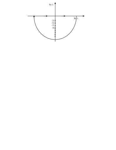
Figure 1: Integration contour along the lower semi-circle for $l=2$.

Hence, due to the residue theorem one obtains

$$\phi(r,\varphi)=-2\pi i\sum_{l=-\infty}^{\infty}\sum_{n=0}^{\infty}\mbox{Res}\,\Psi_{l\lambda}(r,\varphi)\Big{|}_{\lambda=\lambda_{nl}}\,\langle\,\Psi_{l\lambda}|\phi\,\rangle\Big{|}_{\lambda=\lambda_{nl}}\,.$$ (5.22)

Finally, using (5.7) and (5.9) one gets

$$\phi(r,\varphi)=\sum_{l=-\infty}^{\infty}\sum_{n=0}^{\infty}\,\mathfrak{f}^{-}_{nl}(r,\varphi)\,\langle\,\mathfrak{f}^{+}_{nl}|\phi\,\rangle\,.$$ (5.23)

We have proved, therefore, that the subspace ${\cal S}_{-}\subset{\cal S}\subset{\cal H}$ gives rise to the following resolution of identity

$${\mathchoice{\rm 1\mskip-4.0mul}{\rm 1\mskip-4.0mul}{\rm 1\mskip-4.5mul}{\rm 1\mskip-5.0mul}}_{-}\equiv{\mathchoice{\rm 1\mskip-4.0mul}{\rm 1\mskip-4.0mul}{\rm 1\mskip-4.5mul}{\rm 1\mskip-5.0mul}}\Big{|}_{{\cal S}_{-}}\,=\,\sum_{l=-\infty}^{\infty}\sum_{n=0}^{\infty}\,|\mathfrak{f}^{-}_{nl}\,\rangle\langle\,\mathfrak{f}^{+}_{nl}|\,.$$ (5.24)

The same arguments lead us to the following spectral resolution of $\hat{H}$ restricted to ${\cal S}_{-}$:

$$\hat{H}_{-}\equiv\hat{H}\Big{|}_{{\cal S}_{-}}\,=\,\sum_{l=-\infty}^{\infty}\sum_{n=0}^{\infty}\,E^{-}_{nl}\,|\mathfrak{f}^{-}_{nl}\,\rangle\langle\,\mathfrak{f}^{+}_{nl}|\,,$$ (5.25)

with $E^{-}_{nl}$ defined in (5.14). Introducing the following family of operators

$$\hat{P}^{-}_{nl}=|\mathfrak{f}^{-}_{nl}\,\rangle\langle\,\mathfrak{f}^{+}_{nl}|\ ,$$ (5.26)

the spectral decompositions (5.24) and (5.25) may be rewritten as follows

$${\mathchoice{\rm 1\mskip-4.0mul}{\rm 1\mskip-4.0mul}{\rm 1\mskip-4.5mul}{\rm 1\mskip-5.0mul}}_{-}=\sum_{l=-\infty}^{\infty}\sum_{n=0}^{\infty}\,\hat{P}^{-}_{nl}\,,$$ (5.27)

and

$$\hat{H}_{-}=\sum_{l=-\infty}^{\infty}\sum_{n=0}^{\infty}\,E^{-}_{nl}\,\hat{P}^{-}_{nl}\,.$$ (5.28)

Note, that

$$\hat{P}^{-}_{nl}\,\hat{P}^{-}_{n^{\prime}l^{\prime}}=\delta_{nl}\delta_{n^{\prime}l^{\prime}}\,\hat{P}^{-}_{nl}\,,$$ (5.29)

that is, the family $\hat{P}^{-}_{nl}$ seems to play the role of the family of orthogonal projectors. Note, however, that $\hat{P}^{-}_{nl}$ are not hermitian.

6 Time reversal

It was shown in [20] that Bateman’s Hamiltonian is time reversal invariant

$${\cal T}^{\dagger}\hat{H}{\cal T}=\hat{H}\ ,$$ (6.1)

where $\cal T$ denote the anti-unitary time reversal operator. Moreover, it turns out [20] that both $\hat{J}_{0}$ and $\hat{J}_{2}$ satisfy

$${\cal T}^{\dagger}\hat{J}_{0}{\cal T}=\hat{J}_{0}\ ,\hskip 28.45274pt{\cal T}^{\dagger}\hat{J}_{2}{\cal T}=\hat{J}_{2}\ .$$ (6.2)

Let us define

$$\Xi_{l\lambda}={\cal T}\Psi_{l\lambda}\,.$$ (6.3)

In analogy with (4.22) and (4.23) one has the following resolution of identity

$${\mathchoice{\rm 1\mskip-4.0mul}{\rm 1\mskip-4.0mul}{\rm 1\mskip-4.5mul}{\rm 1\mskip-5.0mul}}=\sum_{l=-\infty}^{\infty}\int_{-\infty}^{\infty}\,d\lambda\,|\Xi_{l\lambda}\rangle\langle\Xi_{l\lambda}|\,,$$ (6.4)

and spectral resolution of the Hamiltonian

$$\hat{H}=\sum_{l=-\infty}^{\infty}\int_{-\infty}^{\infty}\,d\lambda\,E_{l\lambda}\,|\Xi_{l\lambda}\rangle\langle\Xi_{l\lambda}|\,.$$ (6.5)

Now, let us introduce another subspace ${\cal S}_{+}$ in the space of test functions

$${\cal S}_{+}=\Big{\{}\phi\in{\cal S}\,\Big{|}\,\langle\,\Xi_{l\lambda}|\phi\,\rangle\in{\cal H}^{2}_{+}\,\Big{\}}\,,$$ (6.6)

that is, $\phi\in{\cal S}_{+}$ iff the complex function

$$\mathbb{C}\ni\lambda\ \longrightarrow\ \langle\,\Xi_{l\lambda}|\phi\,\rangle\,\in\mathbb{C}\ ,$$

is in the Hardy class from above ${\cal H}^{2}_{+}$. It is easy to show that

$${\cal S}_{+}={\cal T}({\cal S}_{-})\ ,$$ (6.7)

and vice versa

$${\cal S}_{-}={\cal T}({\cal S}_{+})\ .$$ (6.8)

Indeed, if $\phi\in{\cal S}_{-}$ then $\langle\,\Psi_{l\lambda}|\phi\,\rangle\in{\cal H}^{2}_{-}$. One has therefore

$$\langle\,\Xi_{l\lambda}|{\cal T}\phi\,\rangle=\langle\,\phi|{\cal T}^{\dagger}\,\Xi_{l\lambda}\,\rangle=\overline{\langle\,\Psi_{l\lambda}|\phi\,\rangle}\in{\cal H}^{2}_{+}\,,$$ (6.9)

which implies that ${\cal T}\phi\in{\cal S}_{+}$. Moreover

$${\cal S}_{-}\cap{\cal S}_{+}=\{\emptyset\}\,.$$ (6.10)

To prove this property let us assume that $\phi\in{\cal S}_{-}\cap{\cal S}_{+}$. Since $\phi\in{\cal S}_{+}$, one has ${\langle\,\Xi_{l\lambda}|\phi\,\rangle}\in{\cal H}^{2}_{+}$. However

$$\langle\,\Xi_{l\lambda}|\phi\,\rangle=\overline{\langle\,\phi|{\cal T}\Psi_{l\lambda}\,\rangle}=\langle\,\Psi_{l\lambda}|{\cal T}^{\dagger}\phi\,\rangle\in{\cal H}^{2}_{+}\,.$$ (6.11)

On the other hand ${\cal T}^{\dagger}\in{\cal S}_{-}$ and hence $\langle\,\Psi_{l\lambda}|{\cal T}^{\dagger}\phi\,\rangle\in{\cal H}^{2}_{-}$. Therefore, $\langle\,\Psi_{l\lambda}|{\cal T}^{\dagger}\phi\,\rangle\in{\cal H}^{2}_{-}\cap{\cal H}^{2}_{+}$ which means that $\langle\,\Psi_{l\lambda}|{\cal T}^{\dagger}\phi\,\rangle$ is en entire function vanishing on the circle $|\lambda|\longrightarrow\infty$. However, any entire function is necessarily bounded and hence such $\phi$ which belongs both to ${\cal S}_{-}$ and ${\cal S}_{+}$ does not exist.

Now, take any test function $\phi\in{\cal S}_{+}$. Formula (6.4) implies

$$\phi(r,\varphi)=\sum_{l=-\infty}^{\infty}\int_{-\infty}^{\infty}d\lambda\,\Xi_{l\lambda}(r,\varphi)\langle\,\Xi_{l\lambda}|\phi\,\rangle\,.$$ (6.12)

Let us continue the eigenvectors $\Xi_{l\lambda}$ for the complex $\lambda$ plane. They have simple poles at $\lambda=-\lambda_{nl}$ with $\lambda_{nl}$ defined in (5.6). The corresponding residues of $\Xi_{l\lambda}$ follows from (5.7)

$${\rm Res}\ \Xi_{l\lambda}\Big{|}_{\lambda=-\lambda_{nl}}=\frac{1}{\sqrt{(|l|+2n)!}}\ \frac{{\cal T}\,\mathfrak{f}^{-}_{nl}}{\sqrt{2\pi}}\ .$$ (6.13)

Moreover,

$$\overline{\Xi_{l\lambda}}\Big{|}_{\lambda=-\lambda_{nl}}=\sqrt{(|l|+2n)!}\ \frac{{\cal T}\overline{\mathfrak{f}^{+}_{nl}}}{\sqrt{2\pi}}\,.$$ (6.14)

Now, since $\langle\,\Xi_{n\lambda}|\phi\,\rangle\in{\cal H}^{2}_{+}$, we may close the integration contour in (6.12) along the upper semi-circle $|\lambda|\rightarrow\infty$. The residue theorem implies

$$\phi(r,\varphi)=2\pi i\sum_{l=-\infty}^{\infty}\sum_{n=0}^{\infty}\mbox{Res}\ \Xi_{l\lambda}(r,\varphi)\Big{|}_{\lambda=-\lambda_{nl}}\,\langle\,\Xi_{l\lambda}|\phi\,\rangle\Big{|}_{\lambda=-\lambda_{nl}}\,.$$ (6.15)

Finally, using (6.13) and (6.14) one gets

$$\phi(r,\varphi)=\sum_{l=-\infty}^{\infty}\sum_{n=0}^{\infty}\,{\cal T}\mathfrak{f}^{-}_{nl}(r,\varphi)\,\overline{\langle\,\phi|{\cal T}\mathfrak{f}^{+}_{nl}}\,\rangle\,,$$ (6.16)

and hence it implies the following resolution of identity on ${\cal S}_{+}$:

$${\mathchoice{\rm 1\mskip-4.0mul}{\rm 1\mskip-4.0mul}{\rm 1\mskip-4.5mul}{\rm 1\mskip-5.0mul}}\Big{|}_{{\cal S}_{+}}\,=\,\sum_{l=-\infty}^{\infty}\sum_{n=0}^{\infty}\,{\cal T}|\mathfrak{f}^{-}_{nl}\,\rangle\langle\,\mathfrak{f}^{+}_{nl}|{\cal T}^{\dagger}\,.$$ (6.17)

Now, the formula (5.12) together with (6.2) gives

$$\hat{J}_{2}\,{\cal T}|\mathfrak{f}^{\pm}_{nl}\rangle=\mp\frac{i}{2}(|l|+2n+1)\,{\cal T}|\mathfrak{f}^{\pm}_{nl}\rangle\ ,$$ (6.18)

and hence one deduces the following relations between $|\mathfrak{f}^{\pm}_{nl}\rangle$ and time reversed ${\cal T}|\mathfrak{f}^{\pm}_{nl}\rangle$

$${\cal T}|\mathfrak{f}^{+}_{nl}\rangle=e^{i\alpha_{nl}}\,|\mathfrak{f}^{-}_{nl}\rangle\,,\hskip 28.45274pt{\cal T}|\mathfrak{f}^{-}_{nl}\rangle=e^{i\alpha_{nl}}\,|\mathfrak{f}^{+}_{nl}\rangle\,,$$ (6.19)

where $\alpha_{nl}$ are arbitrary $(n,l)$-depended phases. It should be stressed that these phases are physically irrelevant. Actually, one may redefine $|\mathfrak{f}^{+}_{nl}\rangle$ in (5.8) and (5.10) such that these additional phase factors disappear from (6.19). Let us observe that

$${\cal T}^{2}|\mathfrak{f}^{\pm}_{nl}\rangle=|\mathfrak{f}^{\pm}_{nl}\rangle\ ,$$ (6.20)

irrespective of $\alpha_{nl}$. Taking into account (6.19) one obtains from (6.17)

$${\mathchoice{\rm 1\mskip-4.0mul}{\rm 1\mskip-4.0mul}{\rm 1\mskip-4.5mul}{\rm 1\mskip-5.0mul}}_{+}\equiv{\mathchoice{\rm 1\mskip-4.0mul}{\rm 1\mskip-4.0mul}{\rm 1\mskip-4.5mul}{\rm 1\mskip-5.0mul}}\Big{|}_{{\cal S}_{+}}\,=\,\sum_{l=-\infty}^{\infty}\sum_{n=0}^{\infty}\,|\mathfrak{f}^{-}_{nl}\,\rangle\langle\,\mathfrak{f}^{+}_{nl}|\,.$$ (6.21)

The same arguments lead us to the following spectral resolution of $\hat{H}$

$$\hat{H}_{+}\equiv\hat{H}\Big{|}_{{\cal S}_{+}}\,=\,\sum_{l=-\infty}^{\infty}\sum_{n=0}^{\infty}\,E^{+}_{nl}\,|\mathfrak{f}^{+}_{nl}\,\rangle\langle\,\mathfrak{f}^{-}_{nl}|\,,$$ (6.22)

with $E^{+}_{nl}$ defined in (5.14). Finally, introducing

$$\hat{P}^{+}_{nl}=|\mathfrak{f}^{+}_{nl}\,\rangle\langle\,\mathfrak{f}^{-}_{nl}|=(\hat{P}^{-}_{nl})^{\dagger}\ ,$$ (6.23)

with $\hat{P}^{-}_{nl}$ defined in (5.26), the spectral decompositions (6.21) and (6.22) may be rewritten as follows

$${\mathchoice{\rm 1\mskip-4.0mul}{\rm 1\mskip-4.0mul}{\rm 1\mskip-4.5mul}{\rm 1\mskip-5.0mul}}_{+}=\sum_{l=-\infty}^{\infty}\sum_{n=0}^{\infty}\,\hat{P}^{+}_{nl}\,,$$ (6.24)

and

$$\hat{H}_{+}=\sum_{l=-\infty}^{\infty}\sum_{n=0}^{\infty}\,E^{+}_{nl}\,\hat{P}^{+}_{nl}\,.$$ (6.25)

7 Resonances and dissipation

What is the physical meaning of the complex eigenvalues $E^{\pm}_{nl}$? To answer this question let us consider the resolvent operator of the Bateman’s Hamiltonian

$$\hat{\rm R}(\hat{H},z)=(\hat{H}-z)^{-1}\,.$$ (7.1)

Using the family of eigenfunctions $|\Psi_{l\lambda}\,\rangle$ one has

$$\hat{\rm R}(\hat{H},z)=\sum_{l=-\infty}^{\infty}\int_{-\infty}^{\infty}\,\,\frac{d\lambda}{E_{l\lambda}-z}\ |\Psi_{l\lambda}\rangle\langle\Psi_{l\lambda}|\,,$$ (7.2)

with $E_{l\lambda}$ defined in (4.16). Now, using the same technique as in Section 5 one easily finds

$$\hat{\rm R}_{-}(z)\equiv\hat{\rm R}(\hat{H},z)\Big{|}_{S_{-}}=\sum_{l=-\infty}^{\infty}\sum_{n=0}^{\infty}\,\frac{1}{E^{-}_{nl}-z}\,\hat{P}^{-}_{nl}\,,$$ (7.3)

with $P^{-}_{nl}$ defined in (5.26). This shows that $E^{-}_{nl}$ constitute poles of the resolvent operator on ${\cal S}_{-}$. In the same way using the family $|\Xi_{l\lambda}\,\rangle$

$$\hat{\rm R}(\hat{H},z)=\sum_{l=-\infty}^{\infty}\int_{-\infty}^{\infty}\,\,\frac{d\lambda}{E_{l\lambda}-z}\ |\Xi_{l\lambda}\rangle\langle\Xi_{l\lambda}|\,,$$ (7.4)

one finds

$$\hat{\rm R}_{+}(z)\equiv\hat{\rm R}(\hat{H},z)\Big{|}_{S_{+}}=\sum_{l=-\infty}^{\infty}\sum_{n=0}^{\infty}\,\frac{1}{E^{+}_{nl}-z}\ \hat{P}^{+}_{nl}\,,$$ (7.5)

which shows that $E^{+}_{nl}$ constitute poles of the resolvent operator on ${\cal S}_{+}$. As is well known [29] the poles of the resolvent operator correspond to resonant states. Hence, the complex eigenvalues $E^{\pm}_{nl}$ may be interpreted as resonances of the Bateman’s Hamiltonian. Note that due to the Cauchy theorem operators $\hat{P}^{\pm}_{nl}$ may be represented by the following integrals

$$\hat{P}^{\pm}_{nl}=\frac{1}{2\pi i}\,\oint_{\gamma^{\pm}_{nl}}\hat{\rm R}_{\pm}(z)\,dz\,,$$ (7.6)

where $\gamma^{\pm}_{nl}$ is any (clockwise) closed curve which encircles a single pole $z=E^{\pm}_{nl}$ (see Figure 2).

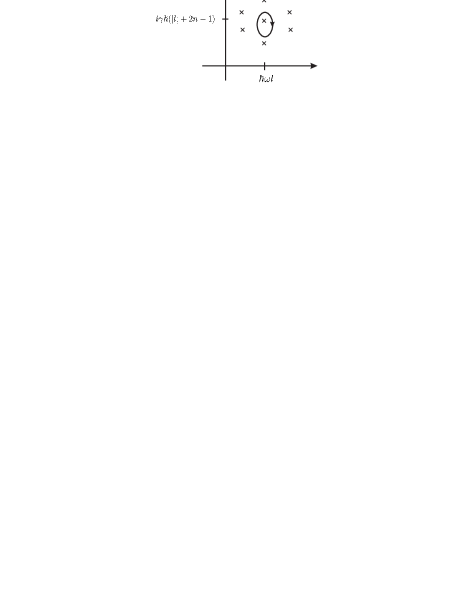
Figure 2: A closed curve $\gamma_{nl}^{+}$ on a complex energy plane.

Finally, let us turn to the evolution generated by the Bateman’s Hamiltonian. Clearly,

$$\mathbb{R}\ni t\ \longrightarrow\ \hat{U}(t)=\exp(-i\hat{H}t/\hbar)\ ,$$

defines a group of unitary operators on the Hilbert space $L^{2}(\mathbb{R}^{2})$. Now, it is easy to see that if $\psi_{-}\in{\cal S}_{-}$, then $\hat{U}(t)\psi_{-}$ belongs to ${\cal S}_{-}$ only if $t\geq 0$. Similarly, if $\psi_{+}\in{\cal S}_{+}$, then $\hat{U}(t)\psi_{+}$ belongs to ${\cal S}_{+}$ only if $t\leq 0$. Therefore, we have two natural semigroups

$$\hat{U}_{-}(t)\ :\ {\cal S}_{-}\ \longrightarrow\ {\cal S}_{-}\ ,\hskip 28.45274pt{\rm for}\ \ t\geq 0\ ,$$ (7.7)

and

$$\hat{U}_{+}(t)\ :\ {\cal S}_{+}\ \longrightarrow\ {\cal S}_{+}\ ,\hskip 28.45274pt{\rm for}\ \ t\leq 0\ ,$$ (7.8)

where

$$\hat{U}_{-}(t)=\hat{U}(t)\Big{|}_{{\cal S}_{-}}\ ,\hskip 19.91684pt{\rm and}\hskip 19.91684pt\hat{U}_{+}(t)=\hat{U}(t)\Big{|}_{{\cal S}_{+}}\ .$$ (7.9)

One has

$$\psi_{-}(t)=\hat{U}_{-}(t)\psi_{-}=\sum_{l=-\infty}^{\infty}e^{-i\omega lt}\,\sum_{n=0}^{\infty}\,e^{-\gamma(|l|+n+1)t}\,\hat{P}^{-}_{nl}\,\psi_{-}\,,$$ (7.10)

for $t\geq 0$, and

$$\psi_{+}(t)=\hat{U}_{+}(t)\psi_{+}=\sum_{l=-\infty}^{\infty}e^{-i\omega lt}\,\sum_{n=0}^{\infty}\,e^{\gamma(|l|+n+1)t}\,\hat{P}^{+}_{nl}\,\psi_{+}\,,$$ (7.11)

for $t\leq 0$. It should be clear that these two semigroups are related by the time reversal operator $\cal T$: indeed formulae (6.19) imply

$${\cal T}\,\hat{P}^{-}_{nl}\,{\cal T}^{\dagger}=\hat{P}^{+}_{nl}\ \hskip 19.91684pt{\rm and}\hskip 19.91684pt{\cal T}\,\hat{P}^{+}_{nl}\,{\cal T}^{\dagger}=\hat{P}^{-}_{nl}\ ,$$ (7.12)

and hence

$${\cal T}\,\hat{U}_{-}(t)\,{\cal T}^{\dagger} = \sum_{l=-\infty}^{\infty}\sum_{n=0}^{\infty}\,{\cal T}\,\left(e^{-iE^{-}_{nl}t/\hbar}\,\hat{P}^{-}_{nl}\right)\,{\cal T}^{\dagger}$$ (7.13)

$$= \sum_{l=-\infty}^{\infty}\sum_{n=0}^{\infty}\,e^{-iE^{+}_{nl}(-t)/\hbar}\,\hat{P}^{+}_{nl}=\hat{U}_{+}(-t)\ ,$$

for $t\geq 0$. Similarly, one finds

$${\cal T}\,\hat{U}_{+}(t)\,{\cal T}^{\dagger}=\hat{U}_{-}(-t)\ ,$$ (7.14)

for $t\leq 0$. We have shown that perfectly reversible quantum dynamics $\hat{U}(t)$ on the full Hilbert space $L^{2}(\mathbb{R}^{2})$ is no longer reversible when restricted to the subspaces ${\cal S}_{-}$ and ${\cal S}_{+}$. This effective irreversibility is caused by the presence of resonant states $|\mathfrak{f}^{\pm}_{nl}\,\rangle$ corresponding to complex eigenvalues $E^{\pm}_{nl}$.

8 Conclusions

In this paper we have studied the spectral properties of the Bateman Hamiltonian. It was shown that the complex eigenvalues $E^{\pm}_{jm}$ given by (2.29) corresponds to the poles of the resolvent operator $\hat{\rm R}(\hat{H},z)=(\hat{H}-z)^{-1}$. Therefore, the corresponding generalized eigenvectors may be interpreted as resonant states of the Bateman dual system. It proves that dissipation and irreversibility is caused by the presence of resonances.

From the mathematical point of view the Bateman system gives rise to the so called Gel’fand triplet or rigged Hilbert space [26, 27] (see also [28, 34]). A Gel’fand triplet (rigged Hilbert space) is a collection of spaces

$$\Phi\subset{\cal H}\subset\Phi^{\prime}\ ,$$ (8.1)

where $\cal H$ is a Hilbert space, $\Phi$ its dense subspace and $\Phi^{\prime}$ is the dual space of continuous linear functionals on $\Phi$. Note, that elements from $\Phi^{\prime}$ do not belong to $\cal H$. This is a typical situation when one deals with the continuum spectrum. The corresponding generalized eigenvectors are no longer elements from the system Hilbert space. They are elements from the dual space $\Phi^{\prime}$, i.e. distributions acting on $\Phi$ [35, 36]. In our case we have two natural Gel’fand triplets:

$${\cal S}_{-}\subset L^{2}(\mathbb{R}^{2})\subset{\cal S}_{-}^{\prime}\ ,$$ (8.2)

and

$${\cal S}_{+}\subset L^{2}(\mathbb{R}^{2})\subset{\cal S}_{+}^{\prime}\ .$$ (8.3)

The first triplet corresponds to the forward dynamics $\hat{U}_{-}$ and the second one corresponds to the backward semigroup $\hat{U}_{+}$. A similar analysis based on rigged Hilbert space approach was performed in [24, 25] for a toy model damped system defned by $\dot{x}=-\gamma x$.

Appendix A

Let us briefly sketch calculations leading to (5.7) and (5.9). We introduce a distribution $\Psi_{l\lambda}$ acting on a test function $\phi(r,\varphi)$ as an antilinear functional defined by the integral

$$\Psi_{l\lambda}(\phi)=\langle\phi|\Psi_{l\lambda}\rangle=\frac{1}{2\pi}\int_{\mathbb{R}^{2}}e^{-il\varphi}r^{-i\lambda-1}\overline{\phi}(r,\varphi)dS=\int_{0}^{\infty}r^{-i\lambda}\overline{\phi}_{l}(r)dr\,,$$ (A.4)

where $\lambda\in\mathbb{C}\,$, $dS=rdr\,d\varphi$, and $\phi_{l}(r)$ is given by (5.2). Expanding $\phi_{l}(r)$ in the power series and rewriting the last integral as

$$\int_{0}^{\infty}r^{-i\lambda}\overline{\phi}_{l}(r)dr = \int_{0}^{1}r^{-i\lambda}\Big{[}\overline{\phi}_{l}(r)-\overline{\phi}_{l}(0)-r\overline{\phi}_{l}^{\prime}(0)-\ldots-\frac{r^{l-1}}{(l-1)!}\overline{\phi}_{l}^{(l-1)}(0)\Big{]}dr$$

$$+ \int_{1}^{\infty}r^{-i\lambda}\overline{\phi}_{l}(r)dr$$

$$+ \int_{0}^{1}r^{-i\lambda}\Big{[}\overline{\phi}_{l}(0)+r\overline{\phi}_{l}^{\prime}(0)+\ldots+\frac{r^{l-1}}{(l-1)!}\overline{\phi}_{l}^{(l-1)}(0)\Big{]}dr\ ,$$

one can observe that the first two summands are regular for all $\lambda\in\mathbb{C}$. The last integral, however, equals to

$$\sum_{k=0}^{l-1}\frac{\overline{\phi}_{l}^{(k)}(0)}{k!}\int_{0}^{1}r^{-i\lambda}r^{k}\,dr=\sum_{k=0}^{l-1}\frac{\overline{\phi}_{l}^{(k)}(0)}{k!}\frac{1}{k-i\lambda+1}$$ (A.6)

and has simple poles in $\lambda_{k}=-i(k+1)$, $k=0,1,\ldots,l-1$. Moreover, one can read from (A.6) that

$${\rm Res}\,\langle\phi|\Psi_{l\lambda}\rangle\Big{|}_{\lambda=-i(k+1)}=\frac{\overline{\phi}_{l}^{(k)}(0)}{k!}.$$ (A.7)

Finally, using

$$\overline{\phi}_{l}^{(k)}(0)=\frac{1}{2\pi}\int_{0}^{2\pi}e^{-il\varphi}\overline{\phi}^{(k)}(0,\varphi)\,d\varphi$$ (A.8)

and

$$\overline{\phi}^{(k)}(0,\varphi)=(-1)^{k}\int_{0}^{\infty}\frac{\delta^{(k)}(r)}{r}\overline{\phi}(r,\varphi)\,rdr\ ,$$ (A.9)

we get

$$\overline{\phi}_{l}^{(k)}(0)=\frac{(-1)^{k}}{2\pi}\int_{\mathbb{R}^{2}}e^{-il\varphi}\frac{\delta^{(k)}(r)}{r}\overline{\phi}(r,\varphi)dS\ .$$ (A.10)

But due to (5.5) in the case investigated here $k=|l|+2n$, hence the poles are located at $\lambda_{nl}=-i(|l|+2n+1)$ and

$${\rm Res}\,\langle\phi|\Psi_{l\lambda}\rangle\Big{|}_{\lambda=\lambda_{nl}}=\frac{1}{\sqrt{(|l|+2n)!}}\frac{\langle\phi|\mathfrak{f}^{-}_{nl}\rangle}{\sqrt{2\pi}}\ ,$$ (A.11)

where $\mathfrak{f}_{nl}^{-}$ is a distribution given by (5.8).

The conjugate distribution $\overline{\Psi_{l\lambda}}$ is defined as

$$\overline{\Psi_{l\lambda}}(\phi)=\langle\phi|\overline{\Psi_{l\lambda}}\rangle=\frac{1}{2\pi}\int_{\mathbb{R}^{2}}e^{il\varphi}r^{i\lambda-1}\overline{\phi}(r,\varphi)dS=\int_{0}^{\infty}r^{i\lambda}\overline{\phi}_{l}(r)dr$$ (A.12)

and it is regular in $\lambda=\lambda_{nl}$. The poles of $\langle\phi|\overline{\Psi}_{l\lambda}\rangle$ are located at $\lambda=\overline{\lambda}_{nl}$. Hence

$$\langle\phi|\overline{\Psi_{l\lambda}}\rangle\Big{|}_{\lambda=\lambda_{nl}}=\sqrt{(|l|+2n)!}\,\frac{\langle\phi|\overline{\mathfrak{f}^{+}_{nl}}\rangle}{\sqrt{2\pi}}\,,$$ (A.13)

where $\mathfrak{f}^{+}_{nl}$ is a distribution given by (5.10).

Appendix B

Let us briefly proof that $\phi_{l}(r)$ given by (5.2) has a power series expansion (5.5) starting from $r^{|l|}$. Supposing that $\phi(x_{1},x_{2})$ is an analytic function

$$\phi(x_{1},x_{2})=\phi(0,0)+\sum_{k_{1},k_{2}}\frac{\partial^{k_{1}+k_{2}}\phi(0,0)}{\partial x_{1}^{k_{1}}\partial x_{2}^{k_{2}}}x_{1}^{k_{1}}x_{2}^{k_{2}}$$ (B.1)

in cartesian coordinates $(x_{1},x_{2})$ it is obvious that in polar $(r,\varphi)$-coordinates one obtains the following expansion for $\phi_{l}(r)$:

$$\phi_{l}(r) = \frac{1}{2\pi}\int_{0}^{2\pi}e^{-il\varphi}\phi(r\cos\varphi,r\sin\varphi)\,d\varphi$$ (B.2)

$$= \frac{1}{2\pi}\int_{0}^{2\pi}e^{-il\varphi}\Big{[}\phi(0,0)+\sum_{k_{1},k_{2}}A_{k_{1},k_{2}}r^{k_{1}+k_{2}}(\cos\varphi)^{k_{1}}(\sin\varphi)^{k_{2}}\Big{]}\,d\varphi$$

$$= \frac{1}{2\pi}\sum_{k_{1},k_{2}}A_{k_{1},k_{2}}r^{k_{1}+k_{2}}\int_{0}^{2\pi}e^{-il\varphi}(\cos\varphi)^{k_{1}}(\sin\varphi)^{k_{2}}\,d\varphi\,,$$

where

$$A_{k_{1},k_{2}}=\frac{\partial^{k_{1}+k_{2}}\phi(0,0)}{\partial x_{1}^{k_{1}}\partial x_{2}^{k_{2}}}\ ,$$

stand for derivatives of $\phi(x_{1},x_{2})$ in $(0,0)$. Now, the question is: for which values of $k\equiv k_{1}+k_{2}$ the sum in (B.2) does not vanish? Clearly, it should be

$$\int_{0}^{2\pi}e^{-il\varphi}(\cos\varphi)^{k_{1}}(\sin\varphi)^{k_{2}}\,d\varphi\neq 0\,.$$ (B.3)

Using the Newton expansions

$$(\cos\varphi)^{k_{1}} = \Big{(}\frac{1}{2}\Big{)}^{k_{1}}\Big{(}e^{i\varphi}+e^{-i\varphi}\Big{)}^{k_{1}}=\Big{(}\frac{1}{2}\Big{)}^{k_{1}}\sum_{m_{1}=0}^{k_{1}}{k_{1}\choose m_{1}}e^{im_{1}\varphi}e^{-i(k_{1}-m_{1})\varphi}\ ,$$

$$(\sin\varphi)^{k_{2}} = \Big{(}\frac{1}{2i}\Big{)}^{k_{2}}\Big{(}e^{i\varphi}-e^{-i\varphi}\Big{)}^{k_{1}}=\Big{(}\frac{1}{2i}\Big{)}^{k_{2}}\sum_{m_{2}=0}^{k_{2}}{k_{2}\choose m_{2}}(-1)^{k_{2}-m_{2}}e^{im_{2}\varphi}e^{-i(k_{2}-m_{2})\varphi}\ ,$$

one can rewrite (B.3) as

$$\Big{(}\frac{1}{2}\Big{)}^{k_{1}}\Big{(}\frac{1}{2i}\Big{)}^{k_{2}}\sum_{m_{1}=0}^{k_{1}}\sum_{m_{2}=0}^{k_{2}}{k_{1}\choose m_{1}}{k_{2}\choose m_{2}}(-1)^{k_{2}-m_{2}}\int_{0}^{2\pi}e^{-i(l+k-2(m_{1}+m_{2}))\varphi}d\varphi\neq 0\ ,$$ (B.4)

hence (B.4) will not vanish iff

$$l+k-2(m_{1}+m_{2})=0\,.$$ (B.5)

Clearly,

$$0\leq m_{1}\leq k_{1}\,,\qquad 0\leq m_{2}\leq k_{2}\,.$$ (B.6)

Now, let $l<0$, so $l=-|l|$ and

$$k=|l|+2(m_{1}+m_{2})=|l|+2n\,,$$ (B.7)

where $n=m_{1}+m_{2}\geq 0$. Due to (B.6), in order to satisfy (B.7) it should be $k\geq|l|$.

On the other hand, if $l>0$, then

$$k=-l+2(m_{1}+m_{2})\leq-l+2k\,,$$ (B.8)

because of (B.6) and finally $k\geq l=|l|$. Note that in this case $k=l+2(m_{1}+m_{2}-l)$, where $m_{1}+m_{2}-l\equiv n\geq 0$.

As a result we obtained that for a given $n$ the lowest power of $r$ in expansion (B.2) is $k_{1}+k_{2}=|l|$. Moreover, in both cases

$$k_{1}+k_{2}=k=|l|+2n\,,\qquad n=0,1,2,\ldots$$ (B.9)

holds.

References

• [1] D.F. Walls, G.J. Millburn, Quantum Optics, Springer, Heildelberg, 1994.
• [2] M.O. Scully, M.S. Zubairy, Quantum Optics, Cambridge University Press, Cambridge 1997.
• [3] M. Sargent III, M.O. Scully, W.E. Lamb Jr., Laser Physics, Addison-Wesley, Reading 1974.
• [4] F. Haake, Statistical treatment of open systems by generalized master equations, Springer, Berlin, 1973.
• [5] E.B. Davies, Quantum Theory of Open Systems, Academic Press, London 1976.
• [6] H.-P. Breuer, F. Petruccione, The Theory of Open Quantum Systems, Oxford University Press, Oxford 2002.
• [7] H. Carmichael, An Open System Approach to Quantum Optics, Springer, Heidelberg 1991.
• [8] R. Alicki, K. Lendi, Quantum Dynamical Semigroups and Applications, Springer, Heidelberg 1987.
• [9] F. Benatti, R. Floreanini (Eds.), Irreversible Quantum Dynamics, Lecture Notes in Physics, Vol. 622, Springer, Berlin 2003.
• [10] P. Garbaczewski, R. Olkiewicz (Eds.), Dynamics of Dissipation, Lecture Notes in Physics, Vol. 597, Springer, Berlin 2003.
• [11] H. Bateman, Phys. Rev. 38, (1931) 815.
• [12] P.M. Morse and H. Feshbach, Methods of Theoretical Physics, vol. 1, McGraw-Hill, New York, 1953.
• [13] F. Boop, Sitz.-Ber. Bayer. Akad. Wiss.,Math.-Natur. Kl. (1973), 67.
• [14] H. Feshbach and Y. Tikochinsky, in: A Festschrift for I.I. Rabi, Trans. New York Ac. Sc. Ser. 2 38, (1977) 44. Y. Tikochinsky, J. Math. Phys. 19 (1978) 888.
• [15] H. Dekker, Phys. Rep. 80, (1981) 1–112.
• [16] E. Celeghini, M. Rasetti and G. Vitiello, Ann. Phys. (N.Y.), 215 (1992) 156–170.
• [17] Y. N. Srivastava, G. Vitiello, Ann. Phys. (N.Y.), 238, (1995) 200–207.
• [18] A. Iorio, G. Vitiello, A. Widom, Ann. Phys. (N.Y.), 241, (1995) 496–506.
• [19] R. Banerjee and P. Mukherjee, J. Phys. A: Math. Gen. 35 (2002) 5591-5598.
• [20] M. Blasone and P. Jizba, Ann. Phys. (N.Y.), 312, (2004) 354–397.
• [21] C.C. Gerry, J. Mat. Phys. 25 (1984) 1820.
• [22] G. ’t Hooft, in: Basics and Highlights of Fundamental Physics, Erice, 1999 [hep-th/0003005].
• [23] M. Blasone, P. Jizba, G. Vitiello, Phys. Lett. A 287 (2001) 205; M. Blasone, E. Celeghini, P. Jizba, G. Vitiello, Phys. Lett. A 310 (2003) 393; M. Blasone, P. Jizba, G. Vitiello, J. Phys. Soc. Jap. 72 (suppl. C) (2003) 50; M. Blasone, P.Jizba, G. Vitiello, in: H.-T. Eltze (Ed.), Decoherence and Entropy in Complex Systems, Lecture Notes in Physics, vol. 633, Springer-Verlag, Berlin, 2003, pp. 151.
• [24] D. Chruściński, J. Math. Phys. 44 (2003) 3718.
• [25] D. Chruściński, J. Math. Phys. 45 (2004) 841.
• [26] I.M. Gel’fand, N.J. Vilenkin, Generalized Functions, Vol. IV, Academic Press, New York, 1964.
• [27] K. Maurin, General Eigenfunction Expansion and Unitary Representations of Topological Groups, PWN, Warszawa, 1968.
• [28] A. Bohm and M. Gadella, Dirac Kets, Gamov Vectors and Gel’fand Triplets, Lecture Notes in Physics 348, Springer, Berlin, 1989.
• [29] S. Albeverio, L.S. Ferreira and L. Streit, eds. Resonances – Models and Phenomena, Lecture Notes in Physics 211, Springer, Berlin, 1984.
• [30] E. Brandas and N. Elander, eds. Resonances, Lecture Notes in Physics 325, Springer, Berlin, 1989.
• [31] L.S. Pontriagin, V.G. Boltańskij, R.V. Gamkrelidze, E.F. Miscenko, The Mathematical Theory of Optimal Precesses, Wiley, New York, 1962.
• [32] I.M. Gel’fand and G.E. Shilov, Generalized functions, Vol. I, Academic Press, New York, 1966; R.P. Kanwal, Generalized Functions: Theory and Techniques, Mathematics in Science and Engineering 177, Academic Press, New York, 1983.
• [33] P.L. Duren, Theory of ${\cal H}^{p}$ Spaces, Academic Press, New York, 1970; P. Koosis, Introduction to $H_{p}$ spaces, London Math. Soc., Lecture Note Series 40, Cambridge University Press, Cambridge, 1980.
• [34] A. Bohm, H.-D. Doebner and P. Kielanowski, Irreversability and Causality, Semigroups and Rigged Hilbert Spaces, Lecture Notes in Physics 504, Springer, Berlin, 1998.
• [35] L. Schwartz, Théorie des distributions, vol. I, Hermann, Paris, 1957
• [36] K. Yosida, Functional Analysis, Springer, Berlin, 1978