Non-local thin films in Casimir force calculations

Abstract

The Casimir force is calculated between plates with thin metallic coating. Thin films are described with spatially dispersive (nonlocal) dielectric functions. For thin films the nonlocal effects are more relevant than for half-spaces. However, it is shown that even for film thickness smaller than the mean free path for electrons, the difference between local and nonlocal calculations of the Casimir force is of the order of a few tenths of a percent. Thus the local description of thin metallic films is adequate within the current experimental precision and range of separations.

I Introduction

The Casimir force between uncharged metallic plates Cas48 (see also reviews Mil94 ; Mos97 ; Kar99 ; Mil01 ; Bor01 ; Mil04 ) attracted considerable attention in the past years. The force was measured in a number of experiments with a high precision using different techniques and geometric configurations Lam97 ; Moh98 ; Roy99 ; Har00 ; Ede00 ; Cha01 ; Bres02 ; Dec03a ; Dec03b . On the other hand, the potential applications of the force in micro and nanomechanics is still largely unexplored. Actuation and nonlinear behavior of a mechanical oscillator with the Casimir force were demonstrated Cha01 and the importance of the force in adhesion and stiction has also been discussed Buk01 ; Joh02 ; Zha03 . Due to technological reasons thin coating layers or multilayered structures are often in use in micromechanical devices. The main question to be addressed in this paper is how important are the nonlocal effects when the film thickness is smaller than the mean free path of the electrons.

For the first time the problem of a thin metallic layer on top of another metal appeared in connection with the first atomic force microscope (AFM) experiments Moh98 ; Roy99 . In these experiments a relatively thick $Al$ layer was covered with $Au/Pd$ film of 20 nm Moh98 or 8 nm Roy99 thick to prevent aluminum oxidation. Because the film was thin enough to be transparent for the light with a characteristic frequency $\omega_{ch}=c/2a$, where $a$ is the distance between the bodies, it was concluded that $Au/Pd$ layer did not influence on the forcefootnote1 . In actual calculations Kli99 the thin $Au/Pd$ film was changed by vacuum. This approach was criticized Sve00a on the basis that according to the Lifshitz formula Lif56 ; LP9 the force depends on the dielectric function $\varepsilon\left(i\zeta\right)$ at imaginary frequencies $\omega=i\zeta$. Kramers-Kronig relation shows that at $\zeta_{ch}=c/2a$ low real frequencies $\omega\ll c/2a$ give significant contribution to $\varepsilon(i\zeta_{ch})$. At low frequencies $Au/Pd$ film is not transparent and it should be taken into account. It was demonstrated that, indeed, even 8 nm thick film gave significant contribution to the force. The calculation in Ref. Kli00 supported this conclusion but the authors speculated that nonlocal effects due to small thickness of the film (smaller than the mean free path for electrons) allowed one to consider the film as transparent.

The question arose again in connection with a recent experiment Lis05 , where the force was measured between a plate and sphere covered with 10 nm or 200 nm $Pd$ film. For thin film the expected reduction of the force was clearly observed. It was indicated that spatial dispersion might be important for calculation of the force in the case of thin film. Also, Boström and Sernelius bostrom2000 pointed out to the need of detailed studies of nonlocal effects, while studying the retarded van der Waals force between thin metallic films within a local approximation.

There have been several works dealing with the problem of nonlocality in the Casimir force between half spaces. Katz katz was the first to point out the need of a quantitative study and in his work only a rough estimate of how spatial dispersion affected dispersive forces was given. Heindricks Heindricks was able to derive Lifshitz formula in an approximate way to include nonlocal effects. Similarly, Dubrava using a phenomenological approach described the Casimir attraction between thin films Dubrava . More recently, based on the formalism of nonlocal optics, the effects for thick metallic layers have been considered. Propagation of bulk plasmons Esq03 ; Esq05 ; Moch05 and electromagnetic response in the region of anomalous dispersion Esq04a were taken into account, showing that the spatial dispersion does not contribute significantly to the Casimir force. The method developed in Ref. Esq04a is very general and can be used for the analysis of all nonlocal effects including those arising in thin films.

II Formalism

The Casimir force between two plates separated by a vacuum gap $a$ at a temperature $T$  is given by the Lifshitz formula Lif56 ; LP9 . The force is expressed via the reflection coefficients $R_{1}$ and $R_{2}$ of the plate 1 and 2, respectively, in the following way:

$$F_{pp}\left(a\right)=-\frac{k_{B}T}{\pi}\sum_{n=0}^{\infty}{}^{\prime}\int\limits_{0}^{\infty}dqqk_{0}\left[\left(R_{1s}^{-1}R_{2s}^{-1}\exp\left(2ak_{0}\right)-1\right)^{-1}+\left(R_{1p}^{-1}R_{2p}^{-1}\exp\left(2ak_{0}\right)-1\right)^{-1}\right],$$ (1)

where subscripts $s$ and $p$ denote the polarization states, ${\bf q}$ is the wave vector along the plates, $q=\left|{\bf q}\right|$, and $k_{0}$ is the normal component of the wave vector defined as

$$k_{0}=\sqrt{\zeta_{n}^{2}/c^{2}+q^{2}}.$$ (2)

In Eq. (1) the sum is calculated over the Matsubara frequencies

$$\zeta_{n}=\frac{2\pi k_{B}T}{\hbar}n.$$ (3)

The reflection coefficients $R_{1}$ and $R_{2}$ are different for $s$ and $p$ polarizations and are functions of $q$ and imaginary frequencies $\zeta_{n}$. They comprise material properties of the plates and for this reason we start our analysis from the reflection coefficients.

II.1 Local case

To set our notation, we first study briefly the known local case, when the optical response depends only on frequency. We start the analysis from a thin film of thickness $h$ on a substrate. It will be assumed here that the film is continuous.

For a film on an infinitely thick substrate the problem is rather simple. The Maxwell equations are solved with the boundary conditions which are the continuity of the tangential components of electric and magnetic fields on both boundaries of the film. The problem can be solved at real frequencies and then analytically continued to the imaginary axis. In the local limit the film and substrate are described by their local dielectric functions which will be denoted as $\varepsilon_{1}\left(\omega\right)$ and $\varepsilon_{2}\left(\omega\right)$. In general, the indexes marking the layers will increase from top to bottom of the plate. The dielectric function of vacuum will be taken as $\varepsilon_{0}\left(\omega\right)=1$. The reflection coefficients in our case are well known in optics. At imaginary frequencies they are Zho95 :

$$R=\frac{r_{01}-r_{21}\exp\left(-2k_{1}h\right)}{1-r_{01}r_{21}\exp\left(-2k_{1}h\right)},$$ (4)

where $r_{ml}$ are the reflection coefficients from the boundary between media $l$ and $m$. These coefficients depend on the polarization, $s$ or $p$, and are defined as

$$r_{ml}^{s}=\frac{k_{m}-k_{l}}{k_{m}+k_{l}},\quad r_{ml}^{p}=\frac{\varepsilon_{l}k_{m}-\varepsilon_{m}k_{l}}{\varepsilon_{l}k_{m}+\varepsilon_{m}k_{l}},$$ (5)

where $k_{m}$ is the normal component of the wave vector in the medium $m$:

$$k_{m}=\sqrt{\varepsilon_{m}\left(i\zeta\right)\frac{\zeta^{2}}{c^{2}}+q^{2}}.$$ (6)

It is easy to check that for $h\rightarrow\infty$ (thick film) $R\rightarrow r_{01}$ and in the opposite limit $h\rightarrow 0$ the reflection coefficient coincides with that for the substrate: $R\rightarrow r_{02}$.

To understand the variation of the Casimir force with the film thickness, we first study the behavior of the reflection coefficients. For a qualitative analysis it will be assumed that a metal, film or substrate, can be described with the Drude dielectric function

$$\varepsilon\left(i\zeta\right)=1+\frac{\omega_{p}^{2}}{\zeta\left(\zeta+\omega_{\tau}\right)},$$ (7)

where $\omega_{p}$ and $\omega_{\tau}$ are the Drude parameters which are different for each layer. For thin films, $\omega_{\tau}$ is a function of the film thickness. This dependence appears because, in addition to the internal scattering processes, for thin films scattering from the surfaces is important. These processes are independent of each other and the relaxation time in the Drude model is $\omega_{\tau}=\omega^{bulk}_{\tau}+\omega^{surf}_{\tau}(h)$. This effect becomes important when the thickness is smaller than the mean free path for electron. Dependence on $h$ of $\omega^{surf}_{\tau}$ is explained by the Fuchs-Sondheimer theory Fuc38 ; Son52 . When $h$ is much smaller than the mean free path, this dependence is given by

$$\omega^{surf}_{\tau}(h)=\frac{3}{8}(1-p)\frac{v_{F}}{h},$$ (8)

where $v_{F}$ is the Fermi velocity and an electron has probability $p$ of being specularly reflected from the surface. As one can see from Eq. (8) only diffusely reflected electrons contribute to $\omega^{surf}_{\tau}(h)$. Experimental results concerning the specularity are far from unique. Very different values of $p$ in the range $0<p<1$ were used to explain the experimental results Fis80 . In this paper we investigate the nonlocal effects for specular reflection of electrons on the surface and do not include in the consideration $h$-dependence of the relaxation frequency. But in any case our results are not very sensitive to the exact value of $\omega_{\tau}$.

Consider first the system consisting of $SiO_{2}$ substrate with $\varepsilon_{2}=4$ and $Au$ film on top of it with the parameters $\omega_{p}=9.0\ eV$, $\omega_{\tau}=0.035\ eV$ Lam00 . It is convenient to introduce dimensionless variables and parameters as follows:

$$\Omega=\frac{\zeta}{\omega_{p}},\ Q=\frac{cq}{\omega_{p}},\ \gamma=\frac{\omega_{\tau}}{\omega_{p}},\ H=\frac{\omega_{p}h}{c}.$$ (9)

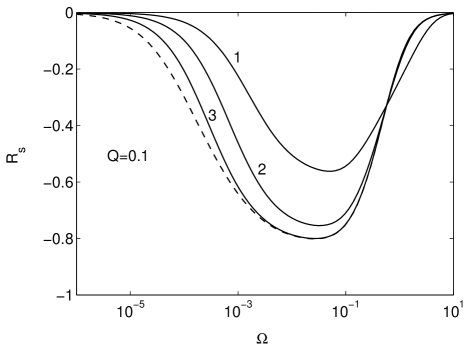
Figure 1: Reflection coefficient for $s$-polarization as a function of $\Omega$ in the local case (metal film on the dielectric substrate). All the results are presented for $Q=0.1$. Infinitely thick film is given by the dashed line. The curves 1, 2, and 3 correspond to the dimensionless thickness $H=0.3$, $1$, and $3$, respectively.

The reflection coefficient for $s$-polarization as a function of the dimensionless frequency $\Omega$ is shown in Fig. 1. The dashed curve corresponds to semi-infinite metal $h\rightarrow\infty$. It was calculated with $Q=0.1$. This value is taken for the characteristic wave number $q\sim 1/2a$ at $a\sim 100\ nm$. The solid lines marked as 1, 2, and 3 correspond to the dimensionless thickness $H=0.3$, $1$, and $3$, respectively. Note that $H=1$ gives the film thickness $h$ equal to the penetration depth $\delta=c/\omega_{p}\approx 22\ nm$ ($Au$). One can see that $R_{s}$ decreases fast with the thickness. When $Q$ increases the film also becomes more transparent for $s$-polarization. The other distinctive feature is that $R_{s}$ is going to zero in the limit $\Omega\rightarrow 0$. In this limit $s$-polarized field degenerates to pure magnetic field, which penetrate freely via the metallic film.

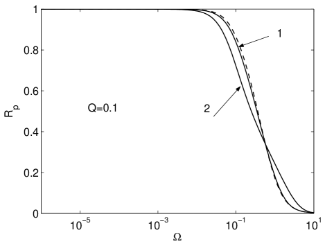
Figure 2: Reflection coefficient for $p$-polarization as a function of $\Omega$ in the local case (metal film on the dielectric substrate). Infinitely thick layer is shown by the dashed line. The solid lines marked as 1 and 2 correspond to $H=1$ and $0.1$, respectively.

The reflection coefficient for $p$-polarization shows a different behavior as one can see in Fig. 2. The dashed line represents the thick film and the solid lines marked as 1 and 2 correspond to $H=1$ and $0.1$, respectively. Variation of $R_{p}$ with the film thickness is not very significant. The reason for this is the effective screening of the $E_{z}$ component even by a very thin metallic layer. An important conclusion can be drawn from this simple fact. The film thickness affects mostly the contribution of $s$-polarization, but the part of the force connected with $p$-polarization is changed weakly in the local case.

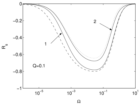
Figure 3: Reflection coefficient for $s$-polarization as a function of $\Omega$ in the local case (metal film on the metallic substrate). The dotted line represents the substrate, $H=0$, the dashed line represents the thick top layer, $H\rightarrow\infty$. The curves 1 and 2 correspond to $H=1$ and $H=0.1$, respectively.

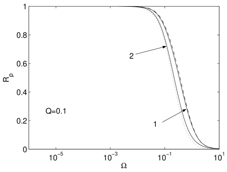
Figure 4: The same as Fig. 3 but for $p$-polarization

Consider now the effect of a thin film on top of a thick metallic layer. It will be assumed that both metals can be described by the Drude dielectric functions $\varepsilon_{1}\left(i\zeta\right)$ and $\varepsilon_{2}\left(i\zeta\right)$ which differ from each other only by the values of parameters $\omega_{ip}$ and $\omega_{i\tau}$ ($i=1,2$). It is clear that in dependence on the film thickness the reflection coefficients will be in between the lines describing metal 1 ($h\rightarrow\infty$) or metal 2 ($h\rightarrow 0$). In Fig. 3 we present the case when the top layer is better reflector than the bottom one. The dotted line gives $r_{02}$ and the dashed line represents $r_{01}$. The results for the film with thickness $H=1$ and $0.1$ are marked as 1 and 2, respectively. In our calculations, the ratios $\omega_{1p}/\omega_{2p}=2$ and $\omega_{1\tau}/\omega_{2\tau}=1$ where used and dimensionless parameters (9) were defined relative to the parameters of the top layer 1. The relaxation frequencies, $\omega_{i\tau}$, influence mostly on low frequency behavior of $R_{s}$. They are not very important for the Casimir force because the main contribution in the force comes from the imaginary frequencies $\Omega\sim c/2a\omega_{p}\gg\gamma$ where $\omega_{\tau}$ does not play significant role. The reflection coefficient, $R_{p}$, for $p$-polarization is shown in Fig. 4. The curves 1 and 2 correspond $H=1$ and $H=0.1$, respectively. Again one can conclude that the top layer is more important for $s$ than for $p$-polarization.

II.2 Nonlocal case

For propagating photons the reflectivity of thin films in the nonlocal case has been analyzed in Ref. Jon69 . It was assumed that electrons are reflected specularly on both boundaries of the film. Let us consider first $s$-polarization. Similar to the case of a semi-infinite metal Kli68 the tangential component of the electric field is considered as even on each boundary:

$$E_{y}\left(mh-z\right)=+E_{y}\left(mh+z\right),$$ (10)

where $z$ is the direction normal to the film surface, $m$ is an arbitrary integer, and the plane of incidence was chosen to be $x-z$. The Maxwell equations and Eq. (10) demand for the magnetic field on the boundaries the following conditions:

$$H_{x}\left(mh-z\right)=-H_{x}\left(mh+z\right),\quad H_{z}\left(mh-z\right)=+H_{z}\left(mh+z\right).$$ (11)

Formally the conditions (10), (11) continue the film of finite thickness to the infinite layer. These conditions mean that the fields can be considered as periodic with period $2h$, and they can be expanded in a Fourier series.

In the nonlocal case the material is characterized by the impedance instead of local dielectric function. The impedance is defined as the ratio of tangential components of electric and magnetic fields just below the surface. For $s$ and $p$-polarizations the impedances of metallic film were found in Ref. Jon69 with the method which is direct generalization of the method used for semi-infinite layer Kli68 . The film has two surfaces and the impedances one can define on each of them:

$$Z_{s}=-\left.\frac{E_{y}}{H_{x}}\right|_{z=\delta,h-\delta},\ Z_{p}=\left.\frac{E_{x}}{H_{y}}\right|_{z=\delta,h-\delta},$$ (12)

where $\delta\rightarrow 0$. It was noted Jon69 that instead of impedances (12) one can use a different couple for each polarization which can be easy calculated. These new impedances were introduced as the ratio of the fields even or odd relative to the film center $z=h/2$. Even or odd fields will be marked by the superscripts $(1)$ or $(2)$, respectively. The new impedances

$$Z_{s}^{(1,2)}=-\left.\frac{E_{y}^{(1,2)}}{H_{x}^{(1,2)}}\right|_{z=\delta},\ Z_{p}^{(1,2)}=\left.\frac{E_{x}^{(1,2)}}{H_{y}^{(1,2)}}\right|_{z=\delta},$$ (13)

are the same on both boundaries of the film because of the symmetry conditions

$$E_{x,y}^{(1)}\left(\delta\right)=E_{x,y}^{(1)}\left(h-\delta\right),\ E_{x,y}^{(2)}\left(\delta\right)=-E_{x,y}^{(2)}\left(h-\delta\right)$$ (14)

and similarly for the magnetic field.

Explicit expressions for these impedances were found in Ref. Jon69 :

$$Z_{s}^{(1,2)}=i\frac{2\omega}{ch}\sum_{n=(odd,\ even)}\frac{1}{\frac{\omega^{2}}{c^{2}}\varepsilon_{t}\left(\omega,k\right)-\left(\frac{n\pi}{h}\right)^{2}-q^{2}},$$ (15)

$$Z_{p}^{(1,2)}=i\frac{2\omega}{ch}\sum_{n=(odd,\ even)}\frac{1}{k^{2}}\left[\frac{q^{2}}{\frac{\omega^{2}}{c^{2}}\varepsilon_{l}\left(\omega,k\right)}+\frac{\left(\frac{n\pi}{h}\right)^{2}}{\frac{\omega^{2}}{c^{2}}\varepsilon_{t}\left(\omega,k\right)-\left(\frac{n\pi}{h}\right)^{2}-q^{2}}\right].$$ (16)

where for even, $(1)$, or odd, $(2)$, fields the sum has to be calculated over $n=2m+1$ or $n=2m$, respectively. The transverse dielectric function $\varepsilon_{t}\left(\omega,k\right)$ contributes to $Z_{s}$. It describes the response of the material on the electric field transverse to the wave vector ${\bf k}$. In case of the $p$-polarization $z$-component of electric field creates a nonzero charge density in the metal producing the longitudinal field inside of metal. That is why $Z_{p}$ depends also on the longitudinal dielectric function $\varepsilon_{l}\left(\omega,k\right)$. In general, these functions are nonlocal, so they depend on both $\omega$ and $k$. The absolute value of the wave vector ${\bf k}$  in Eqs. (15), (16) is

$$k=\sqrt{\left(\frac{n\pi}{h}\right)^{2}+q^{2}}.$$ (17)

Let us consider now the reflection and transmission coefficients of the film on a substrate. Note that in Ref. Jon69 only a free standing film was considered. To find these coefficients one has to match the tangential components of the electric and magnetic fields outside and inside of the film. We assume for simplicity that the substrate can be described by a local dielectric function or equivalently by local impedances. This assumption is justified by the investigation of nonlocal effects at imaginary frequencies for semi-infinite metals Esq04a . It was demonstrated that in contrast with the real frequencies the nonlocal effect (anomalous skin effect) brings only minor influence on the reflection coefficients. Matching the electric field on both sides of the film for $s$-polarization one gets

$$\begin{array}[]{c}E_{y}^{0}\left(1+R_{s}\right)=E_{y}^{(1)}\left(\delta\right)+E_{y}^{(2)}\left(\delta\right),\\ E_{y}^{0}t_{s}e^{ik_{2}h}=E_{y}^{(1)}\left(\delta\right)-E_{y}^{(2)}\left(\delta\right),\end{array}$$ (18)

where $E_{y}^{0}$ is the incident field, $t_{s}$ is the transmission coefficient and the symmetry conditions (14) were taken into account. Similar equations are true for the magnetic field:

$$\begin{array}[]{c}H_{x}^{0}\left(1-R_{s}\right)=H_{x}^{(1)}\left(\delta\right)+H_{x}^{(2)}\left(\delta\right),\\ H_{x}^{0}t_{s}\frac{k_{2}}{k_{0}}e^{ik_{2}h}=-H_{x}^{(1)}\left(\delta\right)+H_{x}^{(2)}\left(\delta\right).\end{array}$$ (19)

Eqs. (18) and (19) can be solved for $R_{s}$ and $t_{s}$ using the impedance definition (13). As the result the reflection coefficient can be presented in the form:

$$R_{s}=\frac{\left(Z_{s1}^{(1)}-Z_{s0}\right)\left(Z_{s1}^{(2)}+Z_{s2}\right)+\left(Z_{s1}^{(2)}-Z_{s0}\right)\left(Z_{s1}^{(1)}+Z_{s2}\right)}{\left(Z_{s1}^{(1)}+Z_{s0}\right)\left(Z_{s1}^{(2)}+Z_{s2}\right)+\left(Z_{s1}^{(2)}+Z_{s0}\right)\left(Z_{s1}^{(1)}+Z_{s2}\right)}.$$ (20)

Here we introduced the following notations : $Z_{s1}^{(1,2)}$ are the nonlocal impedances of the film given by Eq. (13), $Z_{s2}$ is the local impedance of the substrate defined as

$$Z_{s2}=\frac{\omega}{ck_{2}},$$ (21)

and

$$Z_{s0}=\frac{\omega}{ck_{0}},$$ (22)

is the ”impedance” of the plane wave defined as the ratio of electric and magnetic fields in the wave. The formula (20) for $R_{s}$ cannot be presented in the same form (4) as in the local case. This is because we used the impedances (13) instead of that given by Eq. (12). As we will see both Eqs. (4) and (20) coincide in the local limit.

In the same way one can find the reflection coefficient for $p$ -polarization, $R_{p}$. In this case the equations similar to (18), (19) with the interchange $x\leftrightarrow y$ will be true, the impedance of the plane wave is defined as

$$Z_{p0}=\frac{ck_{0}}{\omega}=\frac{1}{Z_{s0}},$$ (23)

and the local impedance of the substrate is

$$Z_{p2}=\frac{ck_{2}}{\omega\varepsilon_{2}\left(\omega\right)}.$$ (24)

The final expression for $R_{p}$ is

$$R_{p}=-\frac{\left(Z_{p1}^{(1)}-Z_{p0}\right)\left(Z_{p1}^{(2)}+Z_{p2}\right)+\left(Z_{p1}^{(2)}-Z_{p0}\right)\left(Z_{p1}^{(1)}+Z_{p2}\right)}{\left(Z_{p1}^{(1)}+Z_{p0}\right)\left(Z_{p1}^{(2)}+Z_{p2}\right)+\left(Z_{p1}^{(2)}+Z_{p0}\right)\left(Z_{p1}^{(1)}+Z_{p2}\right)}.$$ (25)

It differs from Eq. (20) only by the general sign and the change $s\rightarrow p$.

If the substrate is changed by vacuum, $Z_{\alpha 2}\rightarrow Z_{\alpha 0}$ ($\alpha=s,\ p$), we reproduce the reflection coefficient found in Ref. Jon69 :

$$R_{\alpha}=\frac{1}{2}\left(r_{\alpha}^{(1)}+r_{\alpha}^{(2)}\right),\quad\alpha=s,\ p,$$ (26)

where the ”partial” reflection coefficients are connected with the impedances by the usual relations

$$r_{s}^{\left(1,2\right)}=-\frac{Z_{s0}-Z_{s}^{\left(1,2\right)}}{Z_{s0}+Z_{s}^{\left(1,2\right)}},\quad r_{p}^{\left(1,2\right)}=\frac{Z_{p0}-Z_{p}^{\left(1,2\right)}}{Z_{p0}+Z_{p}^{\left(1,2\right)}}.$$ (27)

In the local limit both the transverse $\varepsilon_{t}$ and longitudinal $\varepsilon_{l}$ dielectric functions coincide with the local function: $\varepsilon_{t}\left(\omega,k\right)\rightarrow\varepsilon_{l}\left(\omega,k\right)\rightarrow\varepsilon_{1}\left(\omega\right)$. In this case the sums in Eqs. (15), (16) can be found explicitly. For example, for $s$-polarization one has

$$Z_{1s}^{(1),\ loc}=-i\frac{\omega}{ck_{1}}\tan\frac{hk_{1}}{2},\quad Z_{1s}^{(2),\ loc}=i\frac{\omega}{ck_{1}}\cot\frac{hk_{1}}{2}.$$ (28)

Substituting it in Eq. (20) one can check that the reflection coefficient for the local case given by Eq. (4) is reproduced.

All the equations above were written for real frequencies. Transition to imaginary frequencies, which are the main point of our interest, can be done by a simple analytic continuation. To get the nonlocal effects in the reflection coefficients, we have to fix the nonlocal dielectric functions. At imaginary frequencies in the Boltzmann approximation they are given by the relations Esq04a

$$\varepsilon_{l}\left(\Omega,v\right)=1+\frac{f_{l}\left(v\right)}{\Omega\left(\Omega+\gamma\right)},\quad f_{l}\left(v\right)=\frac{3}{v^{2}}\cdot\frac{v-\arctan v}{v+\frac{\gamma}{\Omega}\left(v-\arctan v\right)},$$ (29)

$$\varepsilon_{t}\left(\Omega,v\right)=1+\frac{f_{t}\left(v\right)}{\Omega\left(\Omega+\gamma\right)},\quad f_{t}\left(v\right)=\frac{3}{2v^{3}}\left[-v+\left(1+v^{2}\right)\arctan v\right],$$ (30)

$$v=\frac{v_{F}}{c}\frac{\sqrt{\left(\frac{n\pi}{H}\right)^{2}+Q^{2}}}{\Omega+\gamma},$$ (31)

where $v_{F}$ is the Fermi velocity. The dimensionless variables (9) have been introduced in Eqs. (29)-(31) . In addition, we have neglected in Eqs. (29) -(30) the contribution due to the interband transitions.

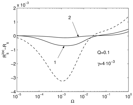
Figure 5: Difference between the reflection coefficients for $s$-polarization in the local and nonlocal cases (metallic film on the dielectric substrate). The dashed curve was calculated for very thick film. The solid curves are presented for $H=1$ (1) and $H=0.1$ (2).

The reflection coefficients in the nonlocal case were calculated numerically. In Fig. 5 the difference between local and nonlocal coefficients $R_{s}$ is shown for $Au$ film on top of $SiO_{2}$ substrate. The dashed curve corresponds to very thick film, $H\rightarrow\infty$. The solid lines marked as 1 and 2 are presented for $H=1$ and 0.1, respectively. As before, $H=1$ corresponds to the penetration depth of $Au$ ($\delta=22$ nm). The thick film clearly demonstrates the anomalous skin effect at $\Omega\sim\gamma$, although the magnitude of the effect is small as was already noted in Ref. Esq04a . Even this small effect decreases with the film thickness as the curves 1 and 2 show. The nonlocal effect increases with $Q$ but it is smaller than 1% even for $Q=1$. It should be noted that the Boltzmann approximation is good while $\Omega<1$, but when $\Omega$ approaching 1 the reflection coefficient itself becomes small and there is no sense to keep the nonlocal correction in this range. Similar result was found for the film on top of a metallic substrate. One can conclude that for $s$-polarization the nonlocal effect in the reflection coefficient is very small and can be neglected in calculation of the Casimir force.

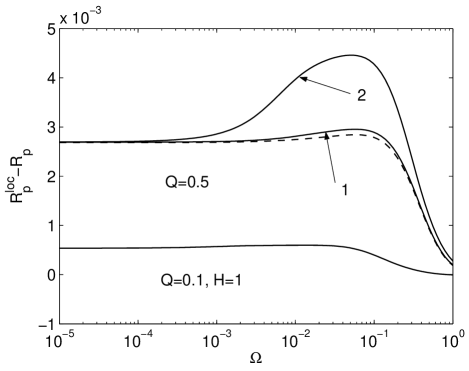
Figure 6: Difference between the reflection coefficients for $p$-polarization in the local and nonlocal cases (metal film on the metallic substrate). The lower line is given for $Q=0.1,H=1$. The upper series is for $Q=0.5$. The dashed curve presents very thick film. The solid curves are given for $H=1$ (1) and $H=0.1$ (2).

The situation for $p$-polarization is shown in Fig. 6 for the film on top of metallic substrate. As in the local case the substrate was chosen to have the plasma frequency 2 times smaller than that for the film. The lower curve corresponds to $Q=0.1$ and $H=1$. The upper series of curves is given for $Q=0.5$. As one can see, the nonlocal effect manifests itself in a wider frequency range and does not disappear even for zero frequency. The latter is the result of Thomas-Fermi screening as was explained in Ref. Esq04a . The effect is still small but the nonlocal contribution in the Casimir force will be larger than that for $s$-polarization. This is because the nonlocal effect is the largest at frequencies which give the main contribution in the Casimir force.

III Effects of Spatial Dispersion on the Casimir force

To quantify the effect of spatial dispersion on the Casimir force, we calculate the percent difference between the local case and nonlocal case ($\Delta\%=|(F_{local}-F_{nonlocal})/F_{local}|$), as a function of separation.

First we consider the case of free standing metallic films. The system is similar to that considered by Boström and Sernelius bostrom2000 . The percent difference $\Delta\%$ as a function of separation is presented in Fig. 7, for three different thicknesses. The results for the thick film $h=100\ nm$ coincides with the results obtained for half spaces in our previous work Esq04a . As the thickness decreases the nonlocal effects become more relevant. Thin films have a more complicated nonlocal response than half spaces. For $p$-polarized waves, surface plasmons on each side of the film can interfere lopez82, creating standing waves that will increase the electromagnetic absorption of the field that will decrease the Casimir force. These resonance conditions are evident from Eq. (17) where $k_{z}=n\pi/L$.

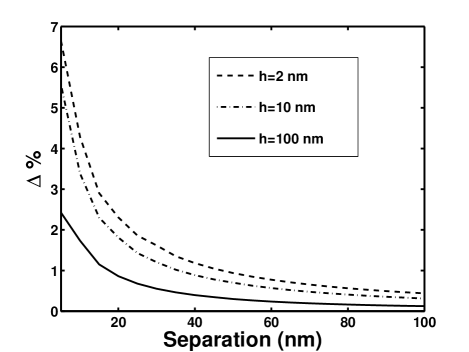
Figure 7: Percent difference $\Delta\%$ between the local and nonlocal Casimir force between $Au$ free standing films. The values for the thick film coincide with those obtained for half-spaces Esq04a .

The force is not affected significantly when the thin films are on substrates. In Figure 8 we have plotted the percent difference between two thin $Au$ films, each deposited on a dielectric substrate. Again, we assumed $\epsilon=4$ for the dielectric, just as an illustrative example of the effect of substrate. The substrates reduce slightly the value of $\Delta\%$ for both curves shown, with the obvious limit that when the substrate has the same dielectric function as the film, we recover the results for the force between half-spaces. This means that the effect of the substrate is to allow energy transfer out of the thin film into the substrate.

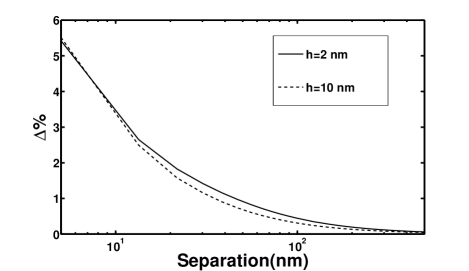
Figure 8: Percent difference $\Delta\%$ between the local and nonlocal Casimir force between two $Au$ films deposited on a dielectric substrate.

The difference between the local and nonlocal cases can be reduced in a system consisting of $Au$ half space and $Au$ coated substrate. Again, we took a dielectric ($\epsilon=4$). The effect of spatial dispersion reduces significantly as compared to the cases treated in Figs. 7 and 8. This shows that the most important part of the spatial dispersion effect come from the thin films. If in current experiments the separation can go down to $50\ nm$, in the system shown in Fig. 9, the nonlocal correction is of the order of $0.34\%$.

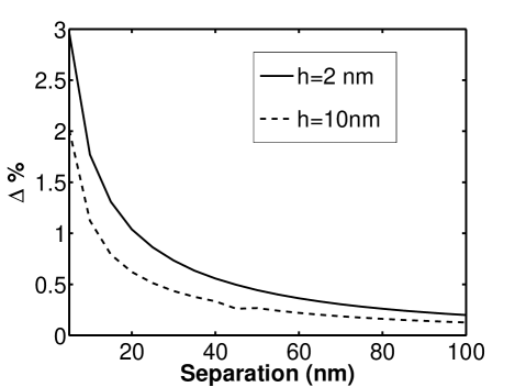
Figure 9: Percent difference $\Delta\%$ between the local and nonlocal Casimir force between $Au$ half space and $Au$ coated dielectric.

The result holds for different substrates. This is shown in Table 1, where we presented the percent difference between the local and nonlocal forces for $Au$ film deposited on different substrates. All data are given for a separation of 50 nm. As before, $\omega_{p1}/\omega_{p2}$ is the ratio of the $Au$ plasma frequency to that of the metallic substrate, assuming the damping factor remains the same. The case $\varepsilon=1$ corresponds to the free standing $Au$ thin film (no substrate).

Table 1: The magnitude of the nonlocal effect for different substrates at a fixed separation of 50 nm and a film thickness of 2 nm.

substrate	$\Delta\%$
dielectric, $\epsilon=4$	0.34
metal, $\frac{\omega_{p1}}{\omega_{p2}}=2$	0.37
metal, $\frac{\omega_{p1}}{\omega_{p2}}=0.5$	0.44
no substrate, $\epsilon=1$	0.44

IV Conclusions

The role of thin metallic coatings in the calculation of Casimir forces has been studied taking into account spatial dispersion. The description of the nonlocal response of thin films is based on the Kliewer and Fuchs formalism that imposes a symmetrical behavior of the fields inside thin films. The study of the reflectivities shows that the main contribution to the nonlocal effect comes from $p$-polarized light that excites normal modes within the material. At very small separations, the effects can be appreciable but at best a percent difference of $7\%$ is found. However, for typical experimental setups and separations the percent difference between the local and nonlocal case is of the order of $0.4\%$, that can be regarded as negligible within current experimental precisions and the local description is good enough. The effect of thin films within a local approximation has been measured recently by Lisanti et al. Lis05 .

Along with the previous works on nonlocal effects between half-spaces Esq03 ; Esq04a ; Esq05 ; Moch05 , we can generally conclude that these effects will be difficult to detect at the current experimental precision. Our results indicate a decrease in the force due to spatial dispersion. However for half-spaces within a jellium model it has been shown Moch05 that the force can increase due to nonlocal effects because of decrease in the separation of the optical surfaces that might not coincide with the physical surface.

- (1) H. B. G. Casimir, Proc. K. Ned. Akad. Wet. 51, 793 (1948).
- (2) P. W. Milonni, The Quantum Vacuum (Academic Press, San Diego, 1994).
- (3) V. M. Mostepanenko and N. N. Trunov, The Casimir Effect and its Applications (Clarendon Press, Oxford, 1997).
- (4) M. Kardar and R. Golestanian, Rev. Mod. Phys. 71, 1233 (1999).
- (5) K. A. Milton, The Casimir Effect (World Scientific, Singapore, 2001).
- (6) M. Bordag, U. Mohideen, and V. M. Mostepanenko, Phys. Rep. 353, 1 (2001).
- (7) K. A. Milton, J. Phys A37, R209 (2004).
- (8) S. K. Lamoreaux, Phys. Rev. Lett. 78, 5 (1997); 81, 5475 (1998).
- (9) U. Mohideen and A. Roy, Phys. Rev. Lett. 81, 4549 (1998).
- (10) A. Roy, C.-Y. Lin, and U. Mohideen, Phys. Rev. D 60, 111101(R) (1999).
- (11) B. W. Harris, F. Chen, and U. Mohideen, Phys. Rev. A 62, 052109 (2000).
- (12) T. Ederth, Phys. Rev. A 62, 062104 (2000).
- (13) H. B. Chan, V. A. Aksyuk, R. N. Kleiman, D. J. Bishop, and F. Capasso, Science 291, 1941 (2001); Phys. Rev. Lett. 87, 211801 (2001).
- (14) G. Bressi, G. Carugno, R. Onofrio, and G. Ruoso, Phys. Rev. Lett. 88, 041804 (2002).
- (15) R. S. Decca, D. López, E. Fischbach, and D. E. Krause, Phys. Rev. Lett. 91, 050402 (2003).
- (16) R. S. Decca, E. Fischbach, G. L. Klimchitskaya, D. E. Krause, D. López, and V. M. Mostepanenko, Phys. Rev. D 68, 116003 (2003).
- (17) E. Buks and M. L. Roukes, Phys. Rev. B 63, 033402 (2001).
- (18) R. W. Johnstone and M. Parameswaran, J. Micromech. Microeng. 12, 855 (2002).
- (19) Y.-P. Zhao, L. S. Wang, and T. X. Yu, J. Adhesion Sci. Technol. 17, 519 (2003).
- (20) For most of the experiments, the force is measured between a large sphere and a plane, being the closest distance between the sphere’s surface and the plane. In the rest of this work we will refer to also as the separation between two parallel planes.
- (21) G. L. Klimchitskaya, A. Roy, U. Mohideen, and V. M. Mostepanenko, Phys. Rev. A 60, 3487 (1999).
- (22) V. B. Svetovoy and M. V. Lokhanin, Mod. Phys. Lett. A 15, 1013 (2000)
- (23) E. M. Lifshitz, Zh. Eksp. Teor. Fiz. 29, 94 (1956) [Sov. Phys. JETP 2, 73 (1956)].
- (24) E. M. Lifshitz and L. P. Pitaevskii, Statistical Physics, Part 2 (Pergamon Press, Oxford, 1980).
- (25) G. L. Klimchitskaya, U. Mohideen, and V. M. Mostepanenko, Phys. Rev. A 61, 062107 (2000).
- (26) M. Lissanti, D. Iannuzzi and F. Capasso, arXiv:quant-ph/0502123v1 (2005).
- (27) D. Iannuzzi, I. Gelfand, M. Lisanti, and F. Capasso, Proc. Quantum Field Theory Under External Conditions 2003, Ed. K. A. Milton (Rynton Press, 2003), p.11; arXiv: quant-ph/0312043.
- (28) D. Iannuzzi, M. Lisanti, and F. Capasso, Proc. Natinonal Acad. Sci. USA, 101, 4019 (2004).
- (29) M. Bostrom and Bo. E. Sernelius, Phys. Rev. B, 62, 7523 (2000).
- (30) E. I. Katz, Sov. Phys. JETP 46, 109 (1977).
- (31) J. Heindricks, Phys. Rev. B 11, 3625 (1975).
- (32) V. N. Dubrava and V. A. Yampolskii, Low Temp. Phys. 25, 979 (1999).
- (33) R. Esquivel, C. Villarreal, W. L. Mochan, Phys. Rev. A 68, 052103 (2003).
- (34) R. Esquivel, C. Villarreal, W. L. Mochan, Phys. Rev. A 71, 029904 (2005).
- (35) A. M. Contreras Reyes, Spatial Dispersion effects in Casimir forces, Thesis, Universidad de las Américas, Puebla (2003) (in spanish).
- (36) R. Esquivel and V. B. Svetovoy, Phys. Rev. A 69, 062102 (2004).
- (37) F. Zhou and L. Spruch, Phys. Rev. A 52, 297 (1995).
- (38) K. Fuchs, Proc. Camb. Philos. Soc. 34, 100 (1938).
- (39) E.H. Sondheimer, Adv. Phys. 1,1 (1952).
- (40) G. Fischer, H. Hoffmann, and J. Vancea, Phys. Rev. B 22, 6065 (1980).
- (41) A. Lambrecht and S. Reynaud, Eur. Phys. J. D 8, 309 (2000).
- (42) W. E. Jones, K. L. Kliewer, and R. Fuchs, Phys. Rev. 178, 1201 (1969).
- (43) K. L. Kliewer and R. Fuchs, Phys. Rev. 172, 607 (1968).
- (44) T. López-Rios, Spatial Dispersion in Solids and Plasmas, Ed. P. Halevi, North-Holland, 217 (1992).