Entanglement and the Power of One Qubit

Abstract

The “Power of One Qubit” refers to a computational model that has access to only one pure bit of quantum information, along with $n$ qubits in the totally mixed state. This model, though not as powerful as a pure-state quantum computer, is capable of performing some computational tasks exponentially faster than any known classical algorithm. One such task is to estimate with fixed accuracy the normalized trace of a unitary operator that can be implemented efficiently in a quantum circuit. We show that circuits of this type generally lead to entangled states, and we investigate the amount of entanglement possible in such circuits, as measured by the multiplicative negativity. We show that the multiplicative negativity is bounded by a constant, independent of $n$, for all bipartite divisions of the $n+1$ qubits, and so becomes, when $n$ is large, a vanishingly small fraction of the maximum possible multiplicative negativity for roughly equal divisions. This suggests that the global nature of entanglement is a more important resource for quantum computation than the magnitude of the entanglement.

I Introduction

Fully controllable and scalable quantum computers are likely many years from realization. This motivates study and development of somewhat less ambitious quantum information processors, defined as devices that fail to satisfy one or more of DiVincenzo’s five criteria for a quantum computer DiVincenzo00 . An example of such a quantum information processor is a mixed-state quantum system, which fails to pass DiVincenzo’s second requirement, that the system be prepared in a simple initial state.

The prime example of a mixed-state quantum information processor is provided by liquid-state NMR experiments in quantum information processing Jones01 . Current NMR experiments, which operate with initial states that are highly mixed thermal states, use a technique called pseudo-pure-state synthesis to process the initial thermal state and thereby to simulate pure-state quantum information processing. This technique suffers from an exponential loss of signal strength as the number of qubits per molecule increases and thus is not scalable. There is a different technique for processing the initial thermal state, called algorithmic cooling Schulman99 , which pumps entropy from a subset of qubits into the remaining qubits, leaving the special subset in a pure state and the remaining qubits maximally mixed. Algorithmic cooling provides an in-principle method for making liquid-state NMR—or any qubit system that begins in a thermal state—scalable, in essence by providing an efficient algorithmic method for cooling a subset of the initially thermal qubits to a pure state, thereby satisfying DiVincenzo’s second criterion.

Knill and Laflamme kl98 proposed a related mixed-state computational model, which they called DQC1, in which there is just one initial pure qubit, along with $n$ qubits in the maximally mixed state. Although provably less powerful than a pure-state quantum computer Ambainis00 , DQC1 can perform some computational tasks efficiently for which there are no known polynomial time classical algorithms. In particular, a DQC1 quantum circuit can be used to evaluate, with fixed accuracy independent of $n$, the normalized trace, ${\rm{tr}}(U_{n})/2^{n}$, of any $n$-qubit unitary operator $U_{n}$ that can be implemented efficiently in terms of quantum gates kl98 ; Laflamme02 . In Sec. II we consider briefly whether there might be efficient classical algorithms for estimating the normalized trace, and we conclude that this is unlikely. The efficient quantum algorithm for estimating the normalized trace provides an exponential speedup over the best known classical algorithm for simulations of some quantum processes pklo04 ; elpc04 . Knill and Laflamme referred to the power of this mixed-state computational model as the “power of one qubit.”

Study of the power of one qubit is motivated partly by NMR experiments, but our primary motivation in this paper is to investigate the role of entanglement in quantum computation, using DQC1 as a theoretical test bed for the investigation. For pure-state quantum computers, Jozsa and Linden Josza99 have shown that exponential speedup over a classical computer requires that entanglement not be restricted to blocks of qubits of fixed size as problem size increases. Entanglement that increases with problem size is thus a necessary prerequisite for the exponential speedup achieved by a pure-state quantum computer. On the other hand, the Gottesman-Knill theorem N&C , demonstrates that global entanglement is far from sufficient for exponential speedup. While this means that the role of entanglement is not entirely understood for pure-state quantum computers, far less is known about the role of entanglement in mixed-state quantum computers. When applied to mixed-state computation, the Jozsa-Linden proof does not show that entanglement is a requirement for exponential speedup. Indeed, it has not previously been shown that there is any entanglement in the DQC1 circuits that provide an exponential speedup over classical algorithms.

The purpose of this paper is to investigate the existence of and amount of entanglement in the DQC1 circuit that is used to estimate the normalized trace. The DQC1 model consists of a special qubit (qubit 0) in the initial state $|0\rangle\langle 0|={1\over 2}(I_{1}+Z)$, where $Z$ is a Pauli operator, along with $n$ other qubits in the completely mixed state, $I_{n}/2^{n}$, which we call the unpolarized qubits. The circuit consists of a Hadamard gate on the special qubit followed by a controlled unitary on the remaining qubits Laflamme02 :

(1)

After these operations, the state of the $n+1$ qubits becomes

$$\rho_{n+1}={1\over 2N}\Bigl{(}|0\rangle\langle 0|\otimes I_{n}+|1\rangle\langle 1|\otimes I_{n}+|0\rangle\langle 1|\otimes U_{n}^{\dagger}+|1\rangle\langle 0|\otimes U_{n}\Bigr{)}=\frac{1}{2N}\begin{pmatrix}I_{n}&\,U_{n}^{\dagger}\\ \,U_{n}&I_{n}\end{pmatrix}\;,$$ (2)

where $N=2^{n}$. The information about the normalized trace of $U_{n}$ is encoded in the expectation values of the Pauli operators $X$ and $Y$ of the special qubit, i.e., $\langle X\rangle={\rm Re}[{\rm{tr}}(U_{n})]/2^{n}$ and $\langle Y\rangle=-{\rm Im}[{\rm{tr}}(U_{n})]/2^{n}$.

To read out the desired information, say, about the real part of the normalized trace, one runs the circuit repeatedly, each time measuring $X$ on the special qubit at the output. The measurement results are drawn from a distribution whose mean is the real part of the normalized trace and whose variance is bounded above by 1. After $L$ runs, one can estimate the real part of the normalized trace with an accuracy $\epsilon\sim 1/\sqrt{L}$. Thus, to achieve accuracy $\epsilon$ requires that the circuit be run $L\sim 1/\epsilon^{2}$ times. More precisely, what we mean by estimating with fixed accuracy is the following: let $P_{e}$ be the probability that the estimate is farther from the true value than $\epsilon\,$; then the required number of runs is $L\sim\ln(1/P_{e})/\epsilon^{2}$. That the number of runs required to achieve a fixed accuracy does not scale with number of qubits and scales logarithmically with the error probability is what is meant by saying that the DQC1 circuit provides an efficient method for estimating the normalized trace.

Throughout much of our analysis, we use a generalization of the DQC1 circuit, in which the initial pure state of the special qubit is replaced by the mixed state ${1\over 2}(I_{1}+\alpha Z)$, which has polarization $\alpha$,

(3)

giving an overall initial state

$$\rho_{i}={1\over 2N}(I_{1}+\alpha Z)\otimes I_{n}={1\over 2N}\!\left[I_{n+1}+\alpha\begin{pmatrix}I_{n}&0\\ 0&-I_{n}\end{pmatrix}\right]\;.$$ (4)

We generally assume that $\alpha\geq 0$, except where we explicitly note otherwise. After the circuit is run, the system state becomes

$$\rho_{n+1}(\alpha)={1\over 2N}\!\left[I_{n+1}+\alpha\begin{pmatrix}0&U_{n}^{\dagger}\\ U_{n}&0\end{pmatrix}\right]=\frac{1}{2N}\begin{pmatrix}I_{n}&\alpha U_{n}^{\dagger}\\ \alpha U_{n}&I_{n}\end{pmatrix}\;.$$ (5)

The effect of subunity polarization is to reduce the expectation values of $\langle X\rangle$ and $\langle Y\rangle$ by a factor of $\alpha$, thereby making it more difficult to estimate the normalized trace. Specifically, the number of runs required to estimate the normalized trace becomes $L\sim\ln(1/P_{e})/\alpha^{2}\epsilon^{2}$. Reduced polarization introduces an additional overhead, but as long as the special qubit has nonzero polarization, the model still provides an efficient estimation of the normalized trace. What we are dealing with is really the “power of even the tiniest fraction of a qubit.”

For $n+1$ qubits, all states contained in a ball of radius $r_{n+1}$ centered at the completely mixed state are separable b99 ; gb03 (distance is measured by the Hilbert-Schmidt norm). Unitary evolution leaves the distance from the completely mixed state fixed, so at all times during the circuit (3), the system state is a fixed distance $\sqrt{{\rm{tr}}(\rho_{i}-I_{n+1}/2N)^{2}}=\alpha 2^{-(n+1)/2}$ from the completely mixed state. This suggests that with $\alpha$ small enough, there might be an exponential speedup with demonstrably separable states. This suggestion doesn’t pan out, however, because the radius of the separable ball decreases exponentially faster than $2^{-(n+1)/2}$. The best known lower bound on $r_{n}$ is $2\times 6^{-n/2}$ gb04 ; for the system state to be contained in a ball given by this lower bound, we need $\alpha\leq 2\times 3^{-(n+1)/2}$. The exponential decrease of $\alpha$ means that an exponentially increasing number of runs is required to estimate the normalized trace with fixed accuracy. More to the point, the possibility that the actual radius of the separable ball might decrease slowly enough to avoid an exponential number of runs is ruled out by the existence of a family of $n$-qubit entangled states found by Dür et al. dur99 , which establishes an upper bound on $r_{n}$ that goes as $2\times 2^{-n}$ for large $n$, implying that $\alpha\leq 2\times 2^{-(n+1)/2}$ if the system state is to be in the ball given by the upper bound. These considerations do not demonstrate the impossibility of an exponential speedup using separable states, but they do rule out the possibility of finding such a speedup within the maximal separable ball about the completely mixed state.

We are thus motivated to look for entanglement in states of the form (5), for at least some unitary operators $U_{n}$. Initial efforts in this direction are not encouraging. It is clear from the start that the marginal state of the $n$ unpolarized qubits remains completely mixed, so these qubits are not entangled among themselves. Moreover, in the state (5), as was shown in Ref. pklo04 , the special qubit is unentangled with the $n$ unpolarized qubits, no matter what $U_{n}$ is used. To see this, one plugs the eigendecomposition of the unitary, $U_{n}=\sum_{j}e^{i\phi_{j}}|e_{j}\rangle\langle e_{j}|$, into the expression for $\rho_{n+1}(\alpha)$. This gives a separable decomposition

$$\rho_{n+1}(\alpha)={1\over 2N}\sum_{j}(|a_{j}\rangle\langle a_{j}|+|b_{j}\rangle\langle b_{j}|)\otimes|e_{j}\rangle\langle e_{j}|\;,$$ (6)

where $|a_{j}\rangle=\cos\theta|0\rangle+e^{i\phi_{j}}\sin\theta|1\rangle$ and $|b_{j}\rangle=\sin\theta|0\rangle+e^{i\phi_{j}}\cos\theta|1\rangle$, with $\sin 2\theta=\alpha$.

No entanglement of the special qubit with the rest and no entanglement among the rest—where then are we to find any entanglement? We look for entanglement relative to other divisions of the qubits into two parts. In such bipartite divisions the special qubit is grouped with a subset of the unpolarized qubits. To detect entanglement between the two parts, we use the Peres-Horodecki partial transpose criterion p96 ; hhh96 , and we quantify whatever entanglement we find using a closely related entanglement monotone which we call the multiplicative negativity Vidal02 . The Peres-Horodecki criterion and the multiplicative negativity do not reveal all entanglement—they can miss what is called bound entanglement—but we are nonetheless able to demonstrate the existence of entanglement in states of the form (2) and (5). For convenience, we generally refer to the multiplicative negativity simply as the negativity. The reader should note, as we discuss in Sec. III, that the term “negativity” was originally applied to an entanglement measure that is closely related to, but different from the multiplicative negativity.

The amount of entanglement depends, of course, on the unitary operator $U_{n}$ and on the bipartite division. We present three results in this regard. First, in Sec. IV, we construct a family of unitaries $U_{n}$ such that for $\alpha>1/2$, $\rho_{n+1}(\alpha)$ is entangled for all bipartite divisions that put the first and last unpolarized qubits in different parts, and we show that for all such divisions, the negativity is $(2\alpha+3)/4$ for $\alpha\geq 1/2$ ($5/4$ for $\alpha=1$), independent of $n$. Second, in Sec. V, we present numerical evidence that the state $\rho_{n+1}$ of Eq. (2) is entangled for typical unitaries, i.e., those created by random quantum circuits. For $n+1=5,\ldots,10$, we find average negativities between 1.155 and just above 1.16 for the splitting that puts $\left\lfloor n/2\right\rfloor$ of the unpolarized qubits with qubit 0. Third, in Sec. VI, we show that for all unitaries and all bipartite divisions of the $n+1$ qubits, the negativity of $\rho_{n+1}(\alpha)$ is bounded above by the constant $\sqrt{1+\alpha^{2}}$ ($\sqrt{2}\simeq 1.414$ for $\alpha=1$), independent of $n$. Thus, when $n$ is large, the negativity achievable by the DQC1 circuit (1) becomes a vanishingly small fraction of the maximum negativity, $\sim 2^{n/2}$, for roughly equal bipartite divisions.

The layout of the paper is as follows. In Sec. II we examine the classical problem of estimating the normalized trace of a unitary. In Sec. III we review pertinent properties of the negativity before applying it to obtain our three key results in Secs. IV-VI. We conclude in Sec. VII and prove a brief Lemma in an Appendix. Throughout we use $\breve{A}$ to stand for the partial transpose of an operator $A$ relative to a particular bipartite tensor-product structure, and we rely on context to make clear which bipartite division we are using at any particular point in the paper.

II Classical Evaluation of the Trace

In this section we outline briefly a classical method for evaluating the trace of a unitary operator that can be implemented efficiently in terms of quantum gates, and we indicate why this appears to be a problem that is exponentially hard in the number of qubits.

The trace of a unitary matrix $U_{n}\equiv U$ is the sum over the diagonal matrix elements of $U$:

$${\rm{tr}}(U)=\sum_{\mathbf{a}}{\langle\mathbf{a}|}U|\mathbf{a}\rangle\;.$$ (7)

Here $\mathbf{a}$ is a bit string that specifies a computational-basis state of the $n$ qubits. By factoring $U$ into a product of elementary gates from a universal set and inserting a resolution of the identity between all the gates, we can write ${\rm{tr}}(U)$ as a sum over the amplitudes of Feynman paths. A difficulty with this approach is that the sum must be restricted to paths that begin and end in the same state. We can circumvent this difficulty by preceding and succeeding $U$ with a Hadamard gate on all the qubits. This does not change the trace, but does allow us to write it as

$${\rm{tr}}(U)=\sum_{\mathbf{a},\mathbf{b},\mathbf{c}}{\langle\mathbf{a}|}H^{\otimes n}|\mathbf{b}\rangle{\langle\mathbf{b}|}U|\mathbf{c}\rangle{\langle\mathbf{c}|}H^{\otimes n}|\mathbf{a}\rangle={1\over 2^{n}}\sum_{\mathbf{a},\mathbf{b},\mathbf{c}}(-1)^{\mathbf{a}\cdot(\mathbf{b}+\mathbf{c})}{\langle\mathbf{b}|}U|\mathbf{c}\rangle\;.$$ (8)

Now if we insert a resolution of the identity between the elementary gates, we get ${\rm{tr}}(U)$ written as an unrestricted sum over Feynman-path amplitudes, with an extra phase that depends on the initial and final states.

Following Dawson et al. dhhmno05 , we consider two universal gate sets: (i) the Hadamard gate $H$, the $\pi/4$ gate $T$, and the controlled-NOT gate and (ii) $H$ and the Toffoli gate. With either of these gate sets, most of the Feynman paths have zero amplitude. Dawson et al. dhhmno05 introduced a convenient method, which we describe briefly now, for including only those paths with nonzero amplitude. One associates with each wire in the quantum circuit a classical bit value corresponding to a computational basis state. The effect of an elementary gate is to change, deterministically or stochastically, the bit values at its input and to introduce a multiplicative amplitude. The two-qubit controlled-NOT gate changes the input control bit $x$ and target bit $y$ deterministically to output values $x$ and $y\oplus x$, while introducing only unit amplitudes. Similarly, the three-qubit Toffoli gates changes the input control bits $x$ and $y$ and target bit $z$ deterministically to $x$, $y$, and $z\oplus xy$, while introducing only unit amplitudes. The $T$ gate leaves the input bit value $x$ unchanged and introduces a phase $e^{ix\pi/4}$. The Hadamard gate changes the input bit value $x$ stochastically to an output value $y$ and introduces an amplitude $(-1)^{xy}/\sqrt{2}$.

The classical bit values trace out the allowed Feynman paths, and the product of the amplitudes introduced at the gates gives the overall amplitude of the path. In our application of evaluating the trace (8), a path is specified by $n$ input bit values (which are identical to the output bit values), $n$ random bit values introduced by the initial Hadamard gates, and $h$ random bit values introduced at the $h$ Hadamard gates required for the implementation of $U$. This gives a total of $2n+h$ bits to specify a path and thus $2^{2n+h}$ allowed paths. We let $\mathbf{x}$ denote collectively the $2n+h$ path bits.

If we apply the gate rules to a Hadamard-Toffoli circuit, the only gate amplitudes we have to worry about are the $\pm 1/\sqrt{2}$ amplitudes introduced at the Hadamard gates. There being no complex amplitudes, the trace cannot be complex. Indeed, for this reason, achieving universality with the $H$-Toffoli gate set requires the use of a simple encoding, and we assume for the purposes of our discussion that this encoding has already been taken into account. With all this in mind, we can write the trace (8) as a sum over the allowed paths,

$${\rm{tr}}(U)=\frac{1}{2^{n+h/2}}\sum_{\mathbf{x}}(-1)^{\psi(\mathbf{x})}\;.$$ (9)

Here $\psi(\mathbf{x})$ is a polynomial over $\mathbb{Z}_{2}$, specifically, the mod-2 sum of the products of input and output bit values at each of the Hadamard gates. The downside is that a string of Toffoli gates followed by a Hadamard can lead to a polynomial that is high order in the bit values. As pointed out by Dawson et al. dhhmno05 , we can deal with this problem partially by putting a pair of Hadamards on the target qubit after each Toffoli gate, thus replacing the quadratic term in the output target bit with two new random variables and preventing the quadratic term from iterating to higher order terms in subsequent Toffoli gates. In doing so, we are left with a cubic term in $\psi(\mathbf{x})$ from the amplitude of the first Hadamard. The upshot is that we can always make $\psi(\mathbf{x})$ a cubic polynomial.

Notice now that we can rewrite the trace as

$${\rm{tr}}(U)=\frac{1}{2^{n+h/2}}\left[\begin{pmatrix}\mbox{number of $\mathbf{x}$ such}\\ \mbox{that $\psi(\mathbf{x})=0$}\end{pmatrix}-\begin{pmatrix}\mbox{number of $\mathbf{x}$ such}\\ \mbox{that $\psi(\mathbf{x})=1$}\end{pmatrix}\right]\;,$$ (10)

thus reducing the problem of evaluating the trace exactly to counting the number of zeroes of the cubic polynomial $\psi(\mathbf{x})$. This is a standard problem from computational algebraic geometry, and it is known that counting the number of zeroes of a general cubic polynomial over any finite field is #P complete ek90 . It is possible that the polynomials that arise from quantum circuits have some special structure that can be exploited to give an efficient algorithm for counting the number of zeroes, but in the absence of such structure, there is no efficient classical algorithm for computing the trace exactly unless the classical complexity hierarchy collapses and all problems in #P are efficiently solvable on a classical computer.

Of course, it is not our goal to compute the trace exactly, since the quantum circuit only provides an efficient method for estimating the normalized trace to fixed accuracy. This suggests that we should estimate the normalized trace by sampling the amplitudes of the allowed Feynman paths. The normalized trace,

$${{\rm{tr}}(U)\over 2^{n}}=\frac{1}{2^{2n+h}}\sum_{\mathbf{x}}2^{h/2}(-1)^{\psi(\mathbf{x})}\;,$$ (11)

which lies between $-1$ and $+1$, can be regarded as the average of $2^{2n+h}$ quantities whose magnitude, $2^{h/2}$, is exponentially large in the number of Hadamard gates. To estimate the average with fixed accuracy requires a number of samples that goes as $2^{h}$, implying that this is not an efficient method for estimating the normalized trace. The reason the method is not efficient is pure quantum mechanics, i.e., that the trace is a sum of amplitudes, not probabilities.

If we apply the gate rules to a Hadamard-$T$-controlled-NOT circuit, the bit value on each wire in the circuit is a mod-2 sum of appropriate bit values in $\mathbf{x}$, but now we have to worry about the amplitudes introduced by the Hadamard and $T$ gates. The trace (8) can be written as

$${\rm{tr}}(U)={1\over 2^{n+h/2}}\sum_{\mathbf{x}}e^{i(\pi/4)\chi(\mathbf{x})}(-1)^{\phi(\mathbf{x})}\;.$$ (12)

Here $\phi(\mathbf{x})$ is a polynomial over $\mathbb{Z}_{2}$, obtained as the mod-2 sum of the products of input and output bit values at each of the Hadamard gates. Since the output value is a fresh binary variable and the input value is a mod-2 sum of bit values in $\mathbf{x}$, $\phi(\mathbf{x})$ is a purely quadratic polynomial over $\mathbb{Z}_{2}$. The function $\chi(\mathbf{x})$ is a mod-8 sum of the input bit values to all of the $T$ gates. Since these input bit values are mod-2 sums of bit values in $\mathbf{x}$, $\chi(\mathbf{x})$ is linear in bit values, but with an unfortunate mixture of mod-2 and mod-8 addition. We can get rid of this mixture by preceding each $T$ gate with a pair of Hadamards, thus making the input to the every $T$ gate a fresh binary variable. With this choice, $\chi(\mathbf{x})$ becomes a mod-8 sum of appropriate bit values from $\mathbf{x}$.

We can rewrite the sum (12) in the following way:

$${\rm{tr}}(U)={1\over 2^{n+h/2}}\sum_{j=0}^{7}e^{i(\pi/4)j}\left[\begin{pmatrix}\mbox{number of $\mathbf{x}$ such that}\\ \mbox{$\chi(\mathbf{x})=j$ and $\phi(\mathbf{x})=0$}\end{pmatrix}-\begin{pmatrix}\mbox{number of $\mathbf{x}$ such that}\\ \mbox{$\chi(\mathbf{x})=j$ and $\phi(\mathbf{x})=1$}\end{pmatrix}\right].$$ (13)

Thus the problem now reduces to finding simultaneous (binary) solutions to the purely quadratic $\mathbb{Z}_{2}$ polynomial $\phi(\mathbf{x})$ and the purely linear $\mathbb{Z}_{8}$ polynomial $\chi(\mathbf{x})$. One has to be careful here to note that we are only interested in binary solutions, so we are not solving $\chi(\mathbf{x})=j$ over all values in $\mathbb{Z}_{8}$. The number of solutions of a purely quadratic polynomial over $\mathbb{Z}_{2}$ can be obtained trivially ek90 , but the constraint over $\mathbb{Z}_{8}$ means that one must count the number of solutions over a mixture of a field and a ring. The complexity class for this problem is not known, but given the equivalence to counting the number of solutions of a cubic polynomial over $\mathbb{Z}_{2}$, it seems unlikely that there is an efficient classical algorithm. Moreover, an attempt to estimate the normalized trace by sampling allowed paths obviously suffers from the problem already identified above.

III Properties of negativity

In this section we briefly review properties of negativity as an entanglement measure, focusing on those properties that we need in the subsequent analysis (for a thorough discussion of negativity, see Ref. Vidal02 ).

Let $A$ be an operator in the joint Hilbert space of two systems, system 1 of dimension $d_{1}$ and system 2 of dimension $d_{2}$. The partial transpose of $A$ with respect to an orthonormal basis of system 2 is defined by taking the transpose of the matrix elements of $A$ with respect to the system-2 indices. A partial transpose can also be defined with respect to any basis of system 1. Partial transposition preserves the trace, and it commutes with taking the adjoint.

The operator that results from partial transposition depends on which basis is used to define the transpose, but these different partial transposes are related by unitary transformations on the transposed system and thus have the same eigenvalues and singular values. Moreover, partial transposition on one of the systems is related to partial transposition on the other by an overall transposition, which also preserves eigenvalues and singular values. Despite the nonuniqueness of the partial transpose, we can talk meaningfully about its invariant properties, such as its eigenvalues and singular values. Similar considerations show that the eigenvalues and singular values are invariant under local unitary transformations.

The singular values of an operator $O$ are the eigenvalues of $\sqrt{O^{\dagger}O}\equiv|O|$ (or, equivalently, of $\sqrt{OO^{\dagger}}$). Any operator has a polar decomposition $O=T|O|$, where $T$ is a unitary operator. Writing $|O|=W^{\dagger}SW$, where $W$ is the unitary that diagonalizes $|O|$ and $S$ is the diagonal matrix of singular values, we see that any operator can be written as $O=VSW$, where $V=TW^{\dagger}$ and $W$ are unitary operators.

We denote a partial transpose of $A$ generically by $\breve{A}$. We write the eigenvalues of $\breve{A}$ as $\lambda_{j}(\breve{A})$ and denote the singular values by $s_{j}(\breve{A})$. If $A$ is Hermitian, so is $\breve{A}$, and the singular values of $\breve{A}$, i.e., the eigenvalues of $|\breve{A}|$, are the magnitudes of the eigenvalues, i.e, $s_{j}(\breve{A})=|\lambda_{j}(\breve{A})|$.

If a joint density operator $\rho$ of systems 1 and 2 is separable, its partial transpose $\breve{\rho}$ is a positive operator. This gives the Peres-Horodecki entanglement criterion p96 ; hhh96 : if $\breve{\rho}$ has a negative eigenvalue, then $\rho$ is entangled (the converse is not generally true). The magnitude of the sum of the negative eigenvalues of the partial transpose, denoted by

$$\mathcal{N}(\rho)\equiv-\sum_{\lambda_{j}(\breve{\rho})<0}\lambda_{j}(\breve{\rho})\;,$$ (14)

is a measure of the amount of entanglement. Partial transposition preserves the trace, so ${\rm{tr}}(\breve{\rho})=1$, from which we get

$$1+2\mathcal{N}(\rho)=\sum_{j}|\lambda_{j}(\breve{\rho})|={\rm{tr}}|\breve{\rho}|\equiv\mathcal{M}(\rho)\;,$$ (15)

where $\mathcal{M}(\rho)$ is a closely related entanglement measure. The quantity $\mathcal{N}(\rho)$ was originally called the negativity Vidal02 ; we can distinguish the two measures by referring to $\mathcal{M}(\rho)$ as the multiplicative negativity, a name that emphasizes one of its key properties and advantages over $\mathcal{N}(\rho)$. In this paper, however, we use the multiplicative negativity exclusively and so refer to it simply as “the negativity”.

The negativity $\mathcal{M}(\rho)$ equals one for separable states, and it is an entanglement monotone Vidal02 , meaning that (i) it is a convex function of density operators and (ii) it does not increase under local operations and classical communication. The negativity has the property of being multiplicative in the sense that the $\mathcal{M}$ value for a state that is a product of states for many pairs of systems is the product of the $\mathcal{M}$ values for each of the pairs. By the same token, $\log\mathcal{M}(\rho)$, called the log-negativity, is additive, but the logarithm destroys convexity so the log-negativity is not an entanglement monotone Vidal02 . For another point of view on the monotonicity of the log-negativity, see Ref. Plenio05 .

The minimum value of the negativity is one, but we need to know the maximum value to calibrate our results. Convexity guarantees that the maximum value is attained on pure states. We can find the maximum SLee03 by considering the Schmidt decomposition of a joint pure state of systems 1 and 2,

$$|\psi\rangle=\sum_{j=1}^{d}\sqrt{\mu_{j}}|j,j\rangle\;,$$ (16)

where $d=\min(d_{1},d_{2})$. Taking the partial transpose of $\rho$ relative to the Schmidt basis of system 2 gives

$$\breve{\rho}=\sum_{j,k=1}^{d}\sqrt{\mu_{j}\mu_{k}}|j,k\rangle\langle k,j|\;,$$ (17)

with eigenvectors and eigenvalues

$$|j,j\rangle\;, \mu_{j}$$ eigenvalue ,

$${1\over\sqrt{2}}(|j,k\rangle\pm|k,j\rangle)\;, \mbox{eigenvalue $\pm\sqrt{\mu_{j}\mu_{k}}$,}\quad j<k.$$ (18)

This gives a negativity

$$\mathcal{M}(\psi)=1+2\sum_{j<k}\sqrt{\mu_{j}\mu_{k}}=\sum_{j,k=1}^{d}\sqrt{\mu_{j}\mu_{k}}=\biggl{(}\sum_{j=1}^{d}\sqrt{\mu_{j}}\biggr{)}^{2}\;.$$ (19)

The concavity of the square root implies $\sum_{j}\sqrt{\mu_{j}}\leq\sqrt{d}$, with equality if and only if $\mu_{j}=1/d$ for all $j$, i.e., $|\psi\rangle$ is maximally entangled. We end up with

$$1\leq\mathcal{M}(\rho)\leq d\;.$$ (20)

The negativity is the sum of the singular values of $\breve{\rho}$. For states of the form we are interested in, given by Eq. (5), the negativity is determined by the singular values of the partial transpose of the unitary operator $U_{n}$. To see this, consider any bipartite division of the qubits. Performing the partial transpose on the part that does not include the special qubit, we have

$$\breve{\rho}_{n+1}(\alpha)=\frac{1}{2N}\begin{pmatrix}I_{n}&\alpha\breve{U}_{n}^{\dagger}\\ \alpha\breve{U}_{n}&I_{n}\end{pmatrix}\;,$$ (21)

where $\breve{U}_{n}$ is the partial transpose of $U_{n}$ relative to the chosen bipartite division. Notice that if we make our division between the special qubit and all the rest, then $\breve{U}_{n}=U_{n}^{T}$ is a unitary operator, and $\breve{\rho}_{n+1}(\alpha)$ is the quantum state corresponding to using $U_{n}^{T}$ in the circuit (3); this shows that for this division, the negativity is 1, consistent with our earlier conclusion that the special qubit is not entangled with the other qubits. For a general division, we know there are unitaries $V$ and $W$ such that $\breve{U}_{n}=VSW$, where $S$ is the diagonal matrix of singular values $s_{j}(\breve{U}_{n})$. This allows us to write

$$\breve{\rho}_{n+1}(\alpha)=\begin{pmatrix}W^{\dagger}&0\\ 0&V\end{pmatrix}\frac{1}{2N}\begin{pmatrix}I_{n}&\alpha S\\ \alpha S&I_{n}\end{pmatrix}\begin{pmatrix}W&0\\ 0&V^{\dagger}\end{pmatrix}\;,$$ (22)

showing that $\breve{\rho}_{n+1}(\alpha)$ is a unitary transformation away from the matrix in the middle and thus has the same eigenvalues. The block structure of the middle matrix makes it easy to find these eigenvalues, which are given by $[1\pm\alpha s_{j}(\breve{U}_{n})]/2N$. This allows us to put the negativity in the form

$$\mathcal{M}\bigl{(}\rho_{n+1}(\alpha)\bigr{)}={1\over 2N}\sum_{j=1}^{N}|1+\alpha s_{j}(\breve{U}_{n})|+|1-\alpha s_{j}(\breve{U}_{n})|={1\over N}\sum_{j=1}^{N}\max\bigl{(}\lvert{\alpha}\rvert s_{j}(\breve{U}_{n}),1\bigr{)}\;,$$ (23)

which is valid for both positive and negative values of $\alpha$. An immediate consequence of Eq. (23) is that $\mathcal{M}\bigl{(}\rho_{n+1}(\alpha)\bigr{)}=\mathcal{M}\bigl{(}\rho_{n+1}(-\alpha)\bigr{)}$, as one would expect. Since $\rho_{n+1}(\alpha)$ is a mixture of $\rho_{n+1}(+1)=\rho_{n+1}$ and $\rho_{n+1}(-1)$, convexity tells us immediately that $\mathcal{M}\bigl{(}\rho_{n+1}(\alpha)\bigr{)}\leq\mathcal{M}\bigl{(}\rho_{n+1}\bigr{)}$, i.e., that a mixed input for the special qubit cannot increase the negativity over that for a pure input. More generally, we have that the negativity cannot decrease at any point as $\alpha$ increases from 0 to 1.

IV Entanglement in the DQC1 Circuit

In this section, we construct a family of unitaries $U_{n}$ that produce global entanglement in the DQC1 circuit (1). For $\alpha=1$, the negativity produced by this family is equal to $5/4$, independent of $n$, for all bipartite divisions that put the first and last unpolarized qubits in different parts. We conjecture that this is the maximum negativity that can be achieved in a circuit of the form (1).

Before the measurement, the output state of the circuit (3) is given by Eq. (5). To construct the unitaries $U_{n}$, we first introduce a two-qubit unitary matrix

$$U_{2}\equiv\begin{pmatrix}A_{1}&C_{1}\\ D_{1}&B_{1}\\ \end{pmatrix}\;,$$ (24)

where $A_{1}$, $B_{1}$, $C_{1}$, and $D_{1}$ are single-qubit ($2\times 2$) matrices that must satisfy $A_{1}^{\dagger}A_{1}+D_{1}^{\dagger}D_{1}=B_{1}^{\dagger}B_{1}+C_{1}^{\dagger}C_{1}=I_{1}$ and $A_{1}^{\dagger}C_{1}+D_{1}^{\dagger}B_{1}=0$ to ensure that $U_{2}$ is unitary. The $n$-qubit unitary $U_{n}$ is then defined by

$$U_{n} \equiv \begin{pmatrix}I_{n-2}\otimes A_{1}&X_{n-2}\otimes C_{1}\\ X_{n-2}\otimes D_{1}&I_{n-2}\otimes B_{1}\end{pmatrix}$$ (25)

$$= |0\rangle\langle 0|\otimes I_{n-2}\otimes A_{1}+|1\rangle\langle 1|\otimes I_{n-2}\otimes B_{1}$$

$$\phantom{|}+|0\rangle\langle 1|\otimes X_{n-2}\otimes C_{1}+|1\rangle\langle 0|\otimes X_{n-2}\otimes D_{1}\;.$$

Here we use $X_{1}$, $Y_{1}$, and $Z_{1}$ to denote single-qubit Pauli operators. A subscript $k$ on the identity operator or a Pauli operator denotes a tensor product in which that operator acts on each of $k$ qubits. If we adopt the convention that $X_{0}=I_{0}=1$, then $U_{n}$ reduces to $U_{2}$ when $n=2$. It is easy to design a quantum circuit that realizes $U_{n}$. The structure of the circuit is illustrated by the case of $U_{4}$:

(26)

In general, the two-qubit unitary $U_{2}$, acting on the first and last qubits, is bracketed by controlled-NOT gates from the first qubit, acting as control, to each of the other qubits, except the last, as targets.

Because $I_{1}$ and $X_{1}$ are invariant under transposition, it is clear from the form of $U_{n}$ that in the state (5), all qubits, except 0, 1, and $n$, are invariant under transposition. We can use this fact to find the negativity for all bipartite divisions. First consider any bipartite division that puts qubits 1 and $n$ in the same part. There are two possibilities. If the special qubit is in the same part as qubits 1 and $n$, then partial transposition on the other part leaves $\rho_{n+1}(\alpha)$ unchanged, so the negativity is 1. If the special qubit is not in the same part as 1 and $n$, then partial transposition on the part that includes 1 and $n$ is the same as partial transposition of all the unpolarized qubits, a case we already know to have negativity equal to 1. We conclude that any bipartite division that puts 1 and $n$ in the same part has negativity equal to 1.

Turn now to bipartite divisions that put qubits 1 and $n$ in different parts. There are two cases to consider: (i) the special qubit is in the same part as qubit 1, and (ii) the special qubit is in the same part as qubit $n$. In case (i), partial transposition of the part that contains qubit $n$ gives

$$\breve{\rho}_{n+1}(\alpha)={1\over 2N}\begin{pmatrix}I_{n}&\alpha\breve{U}_{n}^{\dagger}\\ \alpha\breve{U}_{n}&I_{n}\end{pmatrix}\qquad\mbox{with}\qquad\breve{U}_{n}=\begin{pmatrix}I_{n-2}\otimes A_{1}^{T}&X_{n-2}\otimes C_{1}^{T}\\ X_{n-2}\otimes D_{1}^{T}&I_{n-2}\otimes B_{1}^{T}\end{pmatrix}\;.$$ (27)

In case (ii), partial transposition of the part that contains qubit 1 gives

$$\breve{\rho}_{n+1}(\alpha)={1\over 2N}\begin{pmatrix}I_{n}&\alpha\breve{U}_{n}^{\dagger}\\ \alpha\breve{U}_{n}&I_{n}\end{pmatrix}\qquad\mbox{with}\qquad\breve{U}_{n}=\begin{pmatrix}I_{n-2}\otimes A_{1}&X_{n-2}\otimes D_{1}\\ X_{n-2}\otimes C_{1}&I_{n-2}\otimes B_{1}\end{pmatrix}\;.$$ (28)

The basic structure of $\breve{\rho}_{n+1}(\alpha)$ is the same in both cases. Without changing the spectrum, we can reorder the rows and columns to block diagonalize $\breve{\rho}_{n+1}(\alpha)$ so that there are $N/4$ blocks, each of which has the form

$${1\over 2N}\begin{pmatrix}I_{2}&\alpha\breve{U}_{2}^{\dagger}\\ \alpha\breve{U}_{2}&I_{2}\end{pmatrix}={4\over N}\breve{\rho}_{3}(\alpha)\;,$$ (29)

where $\breve{\rho}_{3}(\alpha)$ is the appropriate partial transpose of the three-qubit output state. Thus the spectrum of $\breve{\rho}_{n+1}(\alpha)$ is the same as the spectrum of $\breve{\rho}_{3}(\alpha)$, except that each eigenvalue is reduced by a factor of $4/N$. In calculating the negativity, since each eigenvalue is ($N/4$)-fold degenerate, the reduction factor of $4/N$ is cancelled by a degeneracy factor of $N/4$, leaving us with the fundamental result of our construction,

$$\mathcal{M}\bigl{(}\rho_{n+1}(\alpha)\bigr{)}=\mathcal{M}\bigl{(}\rho_{3}(\alpha)\bigr{)}\;.$$ (30)

This applies to both cases of bipartite splittings that we are considering, showing that all divisions have the same negativity as the corresponding $n=2$ construction.

We now specialize to a particular choice of $U_{2}$ given by

$$A_{1}=\begin{pmatrix}0&0\\ 0&1\end{pmatrix}\;,\quad B_{1}=\begin{pmatrix}1&0\\ 0&0\end{pmatrix}\;,\quad C_{1}=\begin{pmatrix}0&1\\ 0&0\end{pmatrix}\;,\quad\mbox{and}\quad D_{1}=\begin{pmatrix}0&0\\ 1&0\end{pmatrix}\;.$$ (31)

For this choice, the two cases of bipartite division lead to the same partial transpose. The spectrum of

$$\breve{\rho}_{3}(\alpha)={1\over 8}\begin{pmatrix}I_{1}&0&\alpha A_{1}&\alpha D_{1}\\ 0&I_{1}&\alpha C_{1}&\alpha B_{1}\\ \alpha A_{1}&\alpha D_{1}&I_{1}&0\\ \alpha C_{1}&\alpha B_{1}&0&I_{1}\end{pmatrix}$$ (32)

is

$${\rm{Spec}}(\breve{\rho}_{3}\bigl{(}\alpha)\bigr{)}={1\over 8}(1+2\alpha,1,1,1,1,1,1-2\alpha)\;,$$ (33)

giving a negativity equal to 1 for $\alpha\leq 1/2$ and a negativity

$$\mathcal{M}\bigl{(}\rho_{n+1}(\alpha)\bigr{)}=\mathcal{M}\bigl{(}\rho_{3}(\alpha)\bigr{)}={1\over 4}(2\alpha+3)\quad\mbox{for}\quad\alpha\geq 1/2\;.$$ (34)

This result shows definitively that the circuit  can produce entanglement, at least for $\alpha>1/2$. We stress that the negativity achieved by this family of unitaries is independent of $n\geq 2$.

For $\alpha=1$, the negativity achieved by this family reduces to $5/4$. For large $n$, this amount of negativity is a vanishingly small fraction of the maximum possible negativity, $\sim 2^{n/2}$, for roughly equal divisions of the qubits. This raises the question whether it is possible for other unitaries to achieve larger negativities. A first idea might be to find two-qubit unitaries $U_{2}$ that yield a higher negativity $\mathcal{M}(\rho_{3})=\mathcal{M}(\rho_{n+1})$ when plugged into the construction of this section, but the bounds we find in Sec. VI dispose of this notion, since they show that $5/4$ is the maximum negativity that can be achieved for $n=2$. Another approach would be to generalize the construction of this section in a way that is obvious from the circuit (26), i.e., by starting with a $k$-qubit unitary in place of the two-qubit unitary of Eq. (26). Numerical investigation of the case $k=3$ has not turned up negativities larger than $5/4$. We conjecture that $5/4$ is the maximum negativity that can be achieved by states of the form (2). Though we have not been able to prove this conjecture, we show in the next section that typical unitaries for $n+1\leq 10$ achieve negativities less than $5/4$ and in the following section that the negativity is rigorously bounded by $\sqrt{2}$.

We stress that we are not suggesting that the construction of this section, with $U_{2}$ given by Eq. (31), achieves the maximum negativity for all values of $\alpha$, for that would mean that we believed that the negativity cannot exceed 1 for $\alpha\leq 1/2$, which we do not. Although we have not found entanglement for $\alpha\leq 1/2$, we suspect there are states with negativity greater than 1 as long as $\alpha$ is large enough that $\rho_{n+1}(\alpha)$ lies outside the separable ball around the maximally mixed state, i.e., $\alpha\geq 2^{(n+1)/2}r_{n+1}$. The bound of Sec. VI only says that $\mathcal{M}\bigl{(}\rho_{n+1}(\alpha)\bigr{)}\leq\sqrt{1+\alpha^{2}}$, thus allowing negativities greater than 1 for all values of $\alpha$ except $\alpha=0$. Moreover, since the negativity does not detect bound entanglement, there could be entangled states that have a negativity equal to 1.

V The Average Negativity of a Random Unitary

Having constructed a family of unitaries that yields a DQC1 state with negativity $5/4$, a natural question to ask is, “What is the negativity of a typical state produced by the circuit (1)?” To address this question, we choose the unitary operator in the circuit (1) at random and calculate the negativity. Of course, one must first define what it means for a unitary to be “typical” or “chosen at random”. The natural measure for defining this is the Haar measure, which is the unique left-invariant measure for the group ${\sf U}(N)$ Conway90 . The resulting ensemble of unitaries is known as the Circular Unitary Ensemble, or CUE, and it is parameterized by the Hurwitz decomposition Hurwitz1897 . Although this is an exact parameterization, implementing it requires computational resources that grow exponentially in the size of the unitary Emerson03 . To circumvent this, a pseudo-random distribution that requires resources growing polynomially in the size of the unitary was formulated and investigated in Ref. Emerson03 . This is the distribution from which we draw our random unitaries, and we summarize the procedure for completeness.

We first define a random ${\sf SU}(2)$ unitary as

$$R(\theta,\phi,\chi)=\begin{pmatrix}e^{i\phi}\cos\theta&e^{i\chi}\sin\theta\\ -e^{-i\chi}\sin\theta&e^{-i\phi}\cos\theta\\ \end{pmatrix}\;,$$ (35)

where $\theta$ is chosen uniformly between $0$ and $\pi/2$, and $\phi$ and $\chi$ are chosen uniformly between $0$ and $2\pi$. A random unitary applied to each of the $n$ qubits is then

$${\sf R}=\bigotimes_{i=1}^{n}R(\theta_{i},\phi_{i},\chi_{i})\;,$$ (36)

where a separate random number is generated for each variable at each value of $i$. Now define a mixing operator ${\sf M}$ in terms of nearest-neighbor $Z\otimes Z$ couplings as

$${\sf M}=\exp\left(i\frac{\pi}{4}\sum_{j=1}^{n-1}Z^{(j)}\otimes Z^{(j+1)}\right)\;.$$ (37)

The pseudo-random unitary is then given by

$${\sf R}_{j}{\sf M}{\sf R}_{j-1}\cdots{\sf M}{\sf R}_{2}{\sf M}{\sf R}_{1}\;,$$ (38)

where $j$ is a positive integer that depends on $n$, and each ${\sf R}_{k}$ is chosen randomly as described above. For a given $n$, the larger $j$ is, the more accurately the pseudo-random unitary distribution resembles the actual CUE. From the results in Ref. Emerson03 , $j=40$ gives excellent agreement with the CUE for unitary operators on at least up to 10 qubits, so this is what we use in our calculations.

Due to boundary effects, not all bipartite splittings that put $k$ unpolarized qubits in one part are equivalent. Nevertheless, we consider only bipartite divisions that split the qubits along horizontal lines placed at various points in the circuit of Eq. (1). We refer to the division that groups the last $k$ qubits together as the $(n+1-k,k)$ splitting. For $\alpha=1$, we calculate the average negativity and standard deviation of a pseudo-random state $\rho_{n+1}$ for two different bipartite splittings, $(n,1)$ and $(\left\lfloor n/2\right\rfloor+1,\left\lceil n/2\right\rceil)$. These results are plotted in Fig. 1. For $n+1=5,\ldots,10$, the average negativity for the roughly equal splitting lies between 1.135 and just above 1.16. The standard deviation appears to converge exponentially to zero, as in Ref. Scott03 , a behavior that is typical of asymptotically equivalent matrices. In addition, for $9+1$ qubits, we calculate the average negativity and standard deviation for all nontrivial ($k\neq n$) bipartite splittings $(n+1-k,k)$, and the results are shown in Fig. 2.

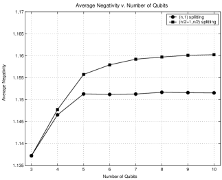
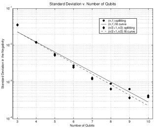
Figure 1: Left: Average negativity of the state $\rho_{n+1}$ of Eq. (2) ($\alpha=1$) for a randomly chosen unitary $U_{n}$ for two different bipartite splittings, $(n,1)$ and $\left(\left\lfloor n/2\right\rfloor+1,\left\lceil n/2\right\rceil\right)$. The $(n,1)$ splitting appears to reach an upper bound quickly, whereas the other splitting is still rising slowly at 10 qubits. Right: Semi-log plot of the standard deviation in the negativity of the randomly chosen state $\rho_{n+1}$. The fit curves show that the standard deviation is decaying exponentially, so that for large numbers of qubits, almost all unitaries give the same negativity.

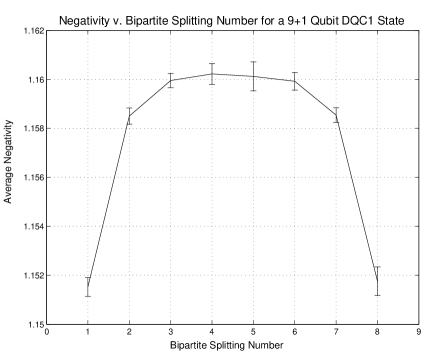
Figure 2: Average negativity of the state $\rho_{10}$ of Eq. (2) ($\alpha=1$) for a randomly chosen unitary $U_{9}$ as a function of bipartite splitting number $k$ for bipartite splittings $(10-k,k)$. The error bars give the standard deviations. The function attains a maximum when the bipartite split is made between half of the qubits on which the unitary acts.

VI Bounds on the Negativity

In this section, we return to allowing the special qubit in the circuit (3) to have initial polarization $\alpha$. Since the value of $n$ is either clear from context or fixed, we reduce the notational clutter by denoting the state $\rho_{n+1}(\alpha)$ of Eq. (5) as $\rho_{\alpha}$.

Given a particular bipartite division, the partial transpose of $\rho_{\alpha}$ with respect to the part that does not include the special qubit is

$$\breve{\rho}_{\alpha}=\frac{I_{n}+\alpha\breve{C}}{2N}\;,$$ (39)

where

$$\breve{C}\equiv\begin{pmatrix}0&\breve{U}_{n}^{\dagger}\\ \breve{U}_{n}&0\end{pmatrix}\;.$$ (40)

Using the binomial theorem, we can expand ${\rm{tr}}(\breve{\rho}^{\,s}_{\alpha})$ in terms of ${\rm{tr}}(\breve{C}^{k})$:

$${\rm{tr}}(\breve{\rho}^{\,s}_{\alpha})=\left({1\over 2N}\right)^{\!\!s}\sum_{k=0}^{s}{s\choose k}\alpha^{k}{\rm{tr}}(\breve{C}^{k})\;.$$ (41)

When $k$ is odd, $\breve{C}^{k}$ is block off-diagonal, so its trace vanishes. When $k$ is even, we have

$${\rm{tr}}(\breve{C}^{k})=2\,{\rm{tr}}\Bigl{(}(\breve{U}_{n}\breve{U}_{n}^{\dagger})^{k/2}\Bigr{)}\;.$$ (42)

When $k=2$, this simplifies to ${\rm{tr}}(\breve{C}^{2})=2{\rm{tr}}(\breve{U}_{n}\breve{U}_{n}^{\dagger})=2{\rm{tr}}(U_{n}U_{n}^{\dagger})=2N$. The crucial step here follows immediately from the property ${\rm{tr}}(\breve{A}\breve{B})={\rm{tr}}(AB)$, which we prove as a Lemma in the Appendix. Note that in general ${\rm{tr}}(\breve{A}_{1}\breve{A}_{2}\ldots\breve{A}_{l})\not={\rm{tr}}(A_{1}A_{2}\ldots A_{l})$ if $l>2$, so we cannot give a similar general calculation of ${\rm{tr}}(\breve{\rho}^{\,s}_{\alpha})$ for even $s\geq 4$, since it involves terms of this form.

Using Eq. (41), we can now obtain three independent constraint equations on the eigenvalues $\lambda_{j}=\lambda_{j}(\breve{\rho}_{\alpha})$ of the partial transpose $\breve{\rho}_{\alpha}$:

$$\sum_{j=1}^{2N}\lambda_{j}^{s}={\rm{tr}}(\breve{\rho}^{\,s}_{\alpha})=\frac{1}{2^{s}N^{s-1}}[(1+\alpha)^{s}+(1-\alpha)^{s}]\;,\qquad s=1,2,3.$$ (43)

Since the negativity is given by

$$\mathcal{M}(\rho_{\alpha})=\sum_{j}\lvert{\lambda_{i}}\rvert\;,$$ (44)

we can find an upper bound on the negativity by maximizing $\sum_{j}\lvert{\lambda_{j}}\rvert$ subject to the constraints (43). If we consider only the $s=1,2$ constraints, we obtain a nontrivial upper bound on the negativity with little effort. We find that adding the constraint $s=3$ adds nothing asymptotically for large $N$, but for small $N$ yields a tighter bound than we get from the $s=1,2$ constraints, although this comes at the cost of considerably more effort. We emphasize that these bounds apply to all bipartite divisions and to all unitaries $U_{n}$. Notice that we have no reason to expect these bounds to be saturated, since the traces of higher powers of $\breve{\rho}_{\alpha}$ impose additional constraints that we are ignoring. The one exception is the case of three qubits, where the $s=1,2,3$ constraints are a complete set, and indeed, in this case, the $s=1,2,3$ bound is $5/4$, which is saturated by the unitary found in Sec. IV.

The remainder of this section is devoted to calculating the $s=1,2$ and $s=1,2,3$ upper bounds. A graphical summary of our results is for $\alpha=1$ presented in Fig. 3.

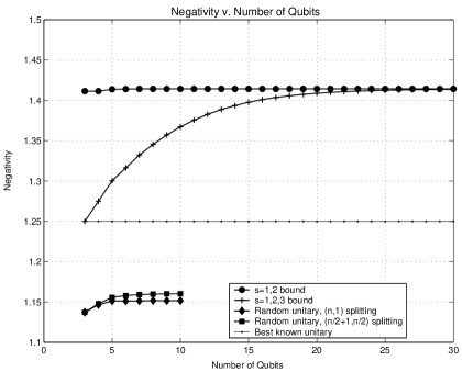
Figure 3: Plot of the bounds on the negativity of states of the form (2), i.e., for a pure-state input in the zeroth register ($\alpha=1$). The uppermost plot is the simple analytic bound $\mathcal{M}_{1,2}=\sqrt{2}$, obtained using the $s=1,2$ constraint equations; the next largest plot is the numerically constructed $s=1,2,3$ bound. One can see that the $s=1,2,3$ bound asymptotes to the $s=1,2$ bound. As noted in the text, these bounds are independent of the unitary $U_{n}$ and the bipartite division. The flat line shows the negativity $5/4$ for the state constructed in Sec. IV, currently the state of the form (2) with the largest demonstrated negativity; notice that for $n+1=3$, this state attains the $s=1,2,3$ bound. The lowest two sets of data points display the expected negativities for a randomly chosen unitary using the bipartite splittings $(n,1)$ and $\left(\left\lfloor n/2\right\rfloor+1,\left\lceil n/2\right\rceil\right)$, which were also plotted in Fig. 1.

VI.1 The $s=1,2$ Bound

We can use Lagrange multipliers to reduce the problem to maximizing a function of one variable, but first we must deal with the absolute value in Eq. (44). To do so, we assume that $t$ of the eigenvalues are negative and the $2N-t$ others are nonnegative, where $t$ becomes a parameter that must now be included in the maximization. We want to maximize

$$\mathcal{M}_{1,2}=-\sum_{i=1}^{t}\lambda_{i}+\sum_{j=t+1}^{2N}\lambda_{j}\;,$$ (45)

subject to the constraints

$$\sum_{k=1}^{2N}\lambda_{k}=1\quad\mbox{and}\quad\sum_{k=1}^{2N}\lambda_{k}^{2}=\frac{1+\alpha^{2}}{2N}\;.$$ (46)

The notation we adopt here for the indices is that $i$ labels negative eigenvalues and $j$ labels nonnegative eigenvalues, while $k$ can label either. This serves to remind us of the sign of an eigenvalue just by looking at its index.

Introducing Lagrange multipliers $\mu$ and $\nu$, the function we want to maximize is

$$f(\lambda_{k},t)=-\sum_{i=1}^{t}\lambda_{i}+\sum_{j=t+1}^{2N}\lambda_{j}+\mu\!\left(\sum_{k=1}^{2N}\lambda_{k}-1\right)+\nu\!\left(\sum_{k=1}^{2N}\lambda_{k}^{2}-\frac{1+\alpha^{2}}{2N}\right)\;.$$ (47)

Differentiating with respect to $\lambda_{i}$ and then $\lambda_{j}$, we find

$$-1+\mu+2\nu\lambda_{i}=0\;,$$ (48)

$$+1+\mu+2\nu\lambda_{j}=0\;.$$ (49)

We immediately see that in the maximal solution, all the negative eigenvalues are equal, and all the nonnegative eigenvalues are equal. We can now reformulate the problem in the following way. If we call the two eigenvalues $\lambda_{-}$ and $\lambda_{+}$, our new problem is to maximize

$$\mathcal{M}_{1,2}=\sum_{k}\lvert{\lambda_{k}}\rvert=-t\lambda_{-}+(2N-t)\lambda_{+}\;,$$ (50)

subject to the constraints

$$t\lambda_{-}+(2N-t)\lambda_{+} = 1\;,$$ (51)

$$t\lambda_{-}^{2}+(2N-t)\lambda_{+}^{2} = \frac{1+\alpha^{2}}{2N}\;.$$ (52)

We can now do the problem by solving the constraints for $\lambda_{-}$ and $\lambda_{+}$ in terms of $t$, plugging these results into $\mathcal{M}_{1,2}$, and then maximizing over $t$.

Before continuing, we note two things. First, $t$ cannot be $2N$, for if it were, then all the eigenvalues would be negative, making it impossible to satisfy Eq. (51). Second, unless $\alpha=0$, $t$ cannot be 0, for if it were, then all the eigenvalues would be equal to $1/2N$ by Eq. (51), a situation Eq. (52) says can occur only if $\alpha=0$. Since we are not really interested in the case $\alpha=0$, for which $\rho_{\alpha}$ is always the maximally mixed state, we assume $\alpha>0$ and $0<t<2N$ in what follows.

Solving Eqs. (51) and (52) and plugging the solutions into Eq. (50), we get the two solutions

$$\mathcal{M}_{1,2}=\frac{N-t\pm\alpha\sqrt{t(2N-t)}}{N}\;.$$ (53)

We choose the positive branch, since it contains the maximum. Maximizing with respect to $t$ treated as a continuous variable, we obtain the upper bound,

$$\mathcal{M}_{1,2}=\sqrt{1+\alpha^{2}}\,\stackrel{{\scriptstyle\alpha\to 1}}{{=}}\sqrt{2}\simeq 1.414\;,$$ (54)

which occurs when the degeneracy parameter is given by

$$t=N\!\left(1-\frac{1}{\sqrt{1+\alpha^{2}}}\right)\stackrel{{\scriptstyle\alpha\to 1}}{{\simeq}}0.292\,N\;.$$ (55)

The numbers on the right are for the case $\alpha=1$, corresponding to the special qubit starting in a pure state. Notice that the upper bound (54) allows a negativity greater than 1 for all $\alpha$ except $\alpha=0$.

Since we did not yet enforce the condition that $t$ be a positive integer, the bound (54) can be made tighter for specific values of $N$ and $\alpha$ by calculating $t$ and checking which of the two nearest integers yields a larger $\mathcal{M}_{1,2}$. Asymptotically, however, the ratio $t/N$ can approach any real number, so this bound for continuous $t$ is the same as the bound for integer $t$ in the limit $N\to\infty$.

VI.2 The $s=1,2,3$ Bound

To deal with this case, we again make the assumption that $t$ of the eigenvalues are negative and $2N-t$ are nonnegative and thus write

$$\mathcal{M}_{1,2,3}=-\sum_{i=1}^{t}\lambda_{i}+\sum_{j=t+1}^{2N}\lambda_{j}\;,$$ (56)

as before. In addition to the constraints (46), we now have a third constraint

$$\sum_{k=1}^{2N}\lambda_{k}^{3}=\frac{1+3\alpha^{2}}{4N^{2}}\;.$$ (57)

We specialize to the case $\alpha=1$ for the remainder of this subsection, because it is our main interest, and the algebra for the general case becomes difficult.

Introducing three Lagrange multipliers, we can write the function we want to maximize as

$$f(\lambda_{k},t)=-\sum_{i=1}^{t}\lambda_{i}+\sum_{j=t+1}^{2N}\lambda_{j}+\mu\!\left(\sum_{k=1}^{2N}\lambda_{k}-1\right)+\nu\!\left(\sum_{k=1}^{2N}\lambda_{k}^{2}-\frac{1}{N}\right)+\xi\!\left(\sum_{k=1}^{2N}\lambda_{k}^{3}-\frac{1}{N^{2}}\right)\;.$$ (58)

Differentiating with respect to $\lambda_{i}$ and then $\lambda_{j}$ gives

$$-1+\mu+2\nu\lambda_{i}+3\xi\lambda_{i}^{2} = 0\;,$$ (59)

$$+1+\mu+2\nu\lambda_{j}+3\xi\lambda_{j}^{2} = 0\;.$$ (60)

These equations being quadratic, we see that there are at most two distinct negative eigenvalues and at most two distinct nonnegative eigenvalues. Since the sum of the two solutions of either of these equations is $-2\nu/3\xi$, however, we can immediately conclude either that one of the potentially nonnegative solutions is negative or that one of the potentially negative solutions is positive. Hence, we find that at least one of the four putative eigenvalues has the wrong sign, implying that there are at most three distinct eigenvalues, though we don’t know whether one or two of them are negative.

Labelling the three eigenvalues by $A$, $B$, and $C$, we can reduce the problem to solving the three constraint equations,

$$uA+vB+wC = 1\;,$$

$$uA^{2}+vB^{2}+wC^{2} = 1/N\;,$$ (61)

$$uA^{3}+vB^{3}+wC^{3} = 1/N^{2}\;,$$

for $A$, $B$, and $C$ and then maximizing $\mathcal{M}_{1,2,3}$ over the degeneracy parameters $u$, $v$, and $w$, which are nonnegative positive integers satisfying the further constraint

$$u+v+w=2N\;.$$ (62)

We do not associate any particular sign with $A$, $B$, and $C$; the signs are determined by the solution of the equations.

One might hope that the symmetry of Eqs. (VI.2) would allow for a simple analytic solution, but this appears not to be the case. In solving the three equations, one is inevitably led to a sixth-order polynomial in one of the variables, with the coefficients given as functions of $u$, $v$, and $w$. Rather than try to solve this equation, which appears intractable, we elected to do a brute force optimization for any given value of $2N$ by solving Eqs. (VI.2) for each possible value of $u$, $v$, and $w$. Picking the solution that has the largest negativity then yields the global maximum. We did this for each $N$ up to $2N=78$. The values of $u$, $v$, and $w$ that maximize the negativity are always

$$u=\left[N\left(1-\frac{1}{\sqrt{2}}\right)\right]\;,\ v=1\;,\ w=2N-1-u\;,$$ (63)

where $[x]$ denotes the integer nearest to $x$. The unique eigenvalue corresponding to $v=1$ is the largest positive eigenvalue, $w$ is the degeneracy of another positive eigenvalue, and $u$ is the degeneracy of the negative eigenvalue. Notice that the degeneracy of the negative eigenvalue is exactly what was found in the $s=1,2$ case. Using the results (63) as a guide, we did a further numerical calculation of the maximum for larger values of $N$, by considering only the area around the degeneracy values given by Eq. (63). While this is not a certifiable global maximum, the perturbation expansion described below matches so well that the two are indistinguishable if they are plotted together for $n+1>7$. This gives us confidence that the numerically determined upper bound $\mathcal{M}_{1,2,3}$, which we plot in Fig. 3, is indeed a global maximum for all $N$.

We have used the numerical work to help formulate a perturbation expansion that gives the first correction to the $N\to\infty$ behavior of the $s=1,2,3$ bound. Defining $x=1/N$, we rewrite the constraint equations (VI.2) as

$$aA+bB+c\,C = x\;,$$

$$aA^{2}+bB^{2}+c\,C^{2} = x^{2}\;,$$ (64)

$$aA^{3}+bB^{3}+c\,C^{3} = x^{3}\;,$$

where $a=u/N$, $b=v/N$, and $c=w/N$. We also have the constraint

$$a+b+c=2\;.$$ (65)

As $x$ is the variable that is asymptotically small, we seek an expansion in terms of it.

Our numerical work tells us that there are two positive eigenvalues, one of which is larger and nondegenerate. In formulating our perturbation expansion, we let $B$ and $C$ be the positive eigenvalues, with $B$ being the larger one, having degeneracy $v=b_{1}\geq 1$. We do not assume that $b_{1}$ is 1, as the numerics show, but rather let the equations force us to that conclusion. With this assumption, the form of the constraints (VI.2) shows that the variables have the following expansions to first order beyond the $N\to\infty$ form:

$$a = a_{0}+a_{1}x^{1/3}\;,$$

$$b = b_{1}x\;,$$ (66)

$$c = c_{0}+c_{1}x^{1/3}\;,$$

and

$$A = A_{0}x+A_{1}x^{4/3}\;,$$

$$B = B_{1}x^{2/3}\;,$$ (67)

$$C = C_{0}x+C_{1}x^{4/3}\;.$$

We see that we are actually expanding in the quantity $y=x^{1/3}$. In terms of these variables, the negativity is given by

$$\mathcal{M}_{1,2,3} = \frac{-aA+bB+cC}{x}$$ (68)

$$= -a_{0}A_{0}+c_{0}C_{0}+(-a_{0}A_{1}-a_{1}A_{0}+c_{0}C_{1}+c_{1}C_{0})x^{1/3}+O(x^{2/3})\;,$$

which we now endeavor to maximize.

Substituting Eqs. (VI.2) and (VI.2) into the constraints (VI.2) and (65) and equating terms with equal exponents of $x$, we obtain, to zero order,

$$a_{0}+c_{0} = 2\;,$$

$$a_{0}A_{0}+c_{0}C_{0} = 1\;,$$ (69)

$$a_{0}A_{0}^{2}+c_{0}C_{0}^{2} = 1\;.$$

Solving for $a_{0}$, $c_{0}$, and $C_{0}$ in terms of $A_{0}$ and substituting the results into the zero-order piece of $\mathcal{M}_{1,2,3}$ gives

$$\mathcal{M}_{1,2,3}=\frac{1-4A_{0}+2A_{0}^{2}}{1-2A_{0}+2A_{0}^{2}}\;.$$ (70)

Maximizing Eq. (70) gives $A_{0}^{2}=1/2$ and, hence, $A_{0}=-1/\sqrt{2}$, since $A$ is the negative eigenvalue. This leads to $a_{0}=1-1/\sqrt{2}$, $c_{0}=1+1/\sqrt{2}$, and $C_{0}=1/\sqrt{2}$, and the resulting $N\to\infty$ upper bound is $\mathcal{M}_{1,2,3}=\sqrt{2}$, as expected.

If we carry this process out to first order beyond the $N\to\infty$ behavior, we obtain, after some algebraic manipulation, $\mathcal{M}_{1,2,3}=\sqrt{2}-b_{1}^{1/3}x^{1/3}/2^{7/6}+O(x^{2/3})$. Maximizing this simply means making $b_{1}$ as small as possible, i.e., choosing $b_{1}=1$, whence we obtain the following asymptotic expression for the $s=1,2,3$ upper bound:

$$\mathcal{M}_{1,2,3}=\sqrt{2}-\frac{1}{2^{7/6}N^{1/3}}+O\!\left(\frac{1}{N^{2/3}}\right)\;.$$ (71)

This shows that the upper bound of $\sqrt{2}$ is approached monotonically from below in the asymptotic regime. In addition, the procedure verifies that in the maximum solution, the largest positive eigenvalue is nondegenerate. For the case of qubits we have $N=2^{n}$, implying that the approach to the $N\to\infty$ bound is exponentially fast.

VII Conclusion

The mixed-state quantum circuit (3) provides an efficient method for estimating the normalized trace of a unitary operator, a task that is thought to be exponentially hard on a classical computer. If one believes that global entanglement is the essential resource for the exponential speedup achieved by quantum computation, then the question begging to be answered is whether there is any entanglement in the circuit’s output state (5). The purpose of this paper was to investigate this question.

A notable feature of the circuit (3) is that it provides an efficient method for estimating the normalized trace no matter how small the initial polarization $\alpha$ of the special qubit in the zeroth register, as long as that polarization is not zero. Since all the other qubits are initially completely unpolarized, we are led to characterize the computational power of this circuit as the “power of even the tiniest fraction of a qubit.” We provide preliminary results regarding the entanglement that can be achieved for $\alpha<1$. Our results are consistent with, but certainly do not demonstrate the conclusion that separable states cannot provide an exponential speedup and that entanglement is possible no matter how small $\alpha$ is. The question of entanglement for subunity polarization of the special qubit deserves further investigation.

Our key conclusions concern the case where the special qubit is initially pure ($\alpha=1$). We find that the circuit (1) typically does produce global entanglement, but the amount of this entanglement is quite small. Using multiplicative negativity to measure the amount of entanglement, we show that as the number of qubits becomes large, the multiplicative negativity in the state (2) is a vanishingly small fraction of the maximum possible multiplicative negativity for roughly equal splittings of the qubits. This hints that the key to computational speedup might be the global character of the entanglement, rather than the amount of the entanglement. In the spirit of the pioneering contribution of Wyler Wyler74 , what happier motto can we find for this state of affairs than Multum ex Parvo, or A Lot out of A Little.

Appendix A Proof of the Lemma

Lemma: ${\rm{tr}}(\breve{A}\breve{B})={\rm{tr}}(AB)$.

Proof: Define two operators $A$ and $B$ by

$$A=\sum_{i,j,k,l}a_{ij,kl}|ij\rangle\!{\langle kl|}\;,\quad B=\sum_{m,n,p,q}b_{mn,pq}|mn\rangle\!{\langle pq|}\;.$$ (72)

Taking the partial transpose with respect to the second subsystem, we find

$$\breve{A}=\sum_{i,j,k,l}a_{ij,kl}|il\rangle\!{\langle kj|}\;,\quad\breve{B}=\sum_{m,n,p,q}b_{mn,pq}|mq\rangle\!{\langle pn|}\;.$$ (73)

Calculating the quantities of interest, we find that they are indeed equal.

$${\rm{tr}}(\breve{A}\breve{B}) = \sum_{\scriptsize\begin{array}[]{l}i,j,k,l,\\ m,n,p,q\end{array}}a_{ij,kl}b_{mn,pq}\langle pn|il\rangle\langle kj|mq\rangle=\sum_{i,j,k,l}a_{ij,kl}b_{kl,ij}\;,$$ (76)

$${\rm{tr}}\left(AB\right) = \sum_{\scriptsize\begin{array}[]{l}i,j,k,l,\\ m,n,p,q\end{array}}a_{ij,kl}b_{mn,pq}\langle pq|ij\rangle\langle kl|mn\rangle=\sum_{i,j,k,l}a_{ij,kl}b_{kl,ij}\;.$$ (79)

References

- (1) D. DiVincenzo, Fortschr. Phys. 48, 9 (2000).
- (2) J. A. Jones, Prog. NMR Spectroscopy 38, 325 (2001).
- (3) L. J. Schulman and U. V. Vazirani, in Proceedings of the 31st Annual ACM Symposium on Theory of Computing (ACM Press, New York, 1999), p. 322 (extended version available as arXiv.org e-print quant-ph/9804060).
- (4) E. Knill and R. Laflamme, Phys. Rev. Lett. 81, 5672 (1998).
- (5) A. Ambainis, L. J. Schulman, and U. V. Vazirani, in Proceedings of the 32nd Annual ACM Symposium on Theory of Computing (ACM Press, New York, 2000), p. 697.
- (6) R. Laflamme, D. G. Cory, C. Negrevergne, and L. Viola, Quant. Inf. Comp. 2, 166 (2002).
- (7) D. Poulin, R. Blume-Kohout, R. Laflamme, and H. Ollivier, Phys. Rev. Lett. 92, 177906 (2004).
- (8) J. Emerson, S. Lloyd, D. Poulin, and D. Cory, Phys. Rev. A 69, 050305(R) (2004).
- (9) R. Josza and N. Linden, Proc. Roy. Soc. Lond. A 459, 2011 (2003).
- (10) M. Nielsen and I. Chuang, Quantum Computation and Quantum Information (Cambridge University Press, Cambridge, England, 2000).
- (11) S. L. Braunstein, C. M. Caves, R. Jozsa, N. Linden, S. Popescu, and R. Schack, Phys. Rev. Lett. 83, 1054 (1999).
- (12) L. Gurvits and H. Barnum, Phys. Rev. A 68, 042312 (2003).
- (13) L. Gurvits and H. Barnum, arXiv.org e-print quant-ph/0409095.
- (14) W. Dür, J. I. Cirac, and R. Tarrach, Phys. Rev. Lett. 83, 3562 (1999).
- (15) A. Peres, Phys. Rev. Lett. 77, 1413 (1996).
- (16) M. Horodecki, P. Horodecki, R. Horodecki, Phys. Lett. A 223, 1 (1996).
- (17) G. Vidal and R. F. Werner, Phys. Rev. A 65, 032314 (2002).
- (18) C. M. Dawson, H. L. Haselgrove, A. P. Hines, D. Mortimer, M. A. Nielsen, and T. J. Osborne, Quant. Inf. Comp. 5, 102 (2005).
- (19) A. Ehrenfeucht and M. Karpinski, Technical Report tr-90-033, International Computer Science Institute, Berkeley, CA (1990), available online at http://www.citeseer.com.
- (20) M. B. Plenio, arXiv.org e-print quant-ph/0505071.
- (21) S. Lee, D. P. Chi, S. D. Oh, and J. Kim, Phys. Rev. A 68, 062304 (2003).
- (22) J. Conway, A Course in Functional Analysis (New York, Springer-Verlag, 1990).
- (23) A. Hurwitz, Nachr. Ges. Wiss. Gött. Math.-Phys. Kl, 71 (1897). The Hurwitz decomposition is discussed in the appendix of M. Poźniak, K. Życzkowski, and M. Kuś, J. Phys. A: Math. Gen. 31, 1059 (1998).
- (24) J. Emerson, Y. S. Weinstein, M. Saraceno, S. Lloyd, and D. G. Cory, Science 302, 2098 (2003).
- (25) A. J. Scott and C. M. Caves, J. Phys. A 36, 9553 (2003).
- (26) J. A. Wyler, Gen. Rel. Grav. 5, 175 (1974).