Engineering Entanglement: The Fast-Approach Phase Gate

Abstract

Optimal-control techniques and a fast-approach scheme are used to implement a collisional control phase gate in a model of cold atoms in an optical lattice, significantly reducing the gate time as compared to adiabatic evolution while maintaining high fidelity. New objective functionals are given for which optimal paths are obtained for evolution that yields a control-phase gate up to single-atom Rabi shifts. Furthermore, the fast-approach procedure is used to design a path to significantly increase the fidelity of non-adiabatic transport in a recent experiment. Also, the entanglement power of phase gates is quantified.

I Introduction

Quantum information processing with cold atoms in optical lattices Jaksch_98 ; deutsch98 ; Brennen_99 ; Jaksch_99 ; Calarco ; Tiesinga ; 1dim and in micro-traps Jaksch_99 ; Calarco ; Eckert_02 ; Dumke_02 rely on the ability to entangle nearest neighbor atoms in an efficient controlled way. The effective trapping potential in optical lattices can have the form of a double well where the distance between minima, the well separation height, the frequency of each well, etc., can each be manipulated by controlling the lasers, using different combinations of laser frequencies and bias fields Guidoni_99 . Ideally each atom is initially in one of the optical wells, and single qubits are registered into each atom’s state. The atom’s internal states (e.g., hyperfine levels) Brennen_99 ; Jaksch_99 or motional states in the trap Eckert_02 ; Tiesinga can be used as a computational basis, $|n\rangle$, where $n=0,1$. A two-qubit gate is implemented by bringing the atoms together and letting their wave functions overlap Brennen_99 ; Jaksch_99 ; Calarco ; Eckert_02 ; Tiesinga ; 1dim ; Bloch . During this overlap a phase that depends on the two-qubits state, $|m,n\rangle\equiv|m\rangle\otimes|n\rangle$, is accumulated because of the atom-atom (molecular) interaction. Two-qubit phase gates based on this scheme were suggested Brennen_99 ; Jaksch_99 ; Calarco , analyzed Calarco ; Eckert_02 ; Tiesinga ; 1dim , and demonstrated Bloch .

To achieve efficient computation and to be faster than decoherence processes, it is desirable to generate gates which operate as fast as possible Robin ; phystoday . Cirac and Zoller phystoday discuss the slow two-qubit collisional gate as one among two serious obstacles (the other is decoherence) to quantum computing with atoms in optical potentials. In designing a fast collisional gate one is faced with the problem of leakage outside the computational subspace due to rapid switching of the control parameters. A theoretical question with immediate practical impact on the feasibility of quantum computation emerges: how fast can such a gate be? Previous theoretical work used adiabatic evolution to ensure the fidelity of the gate. In a recent experimental implementation Bloch , the time scale for motion, 40 $\mu$s, was chosen “to avoid any vibrational excitations”.

Designing a fast two-qubit collisional gate is the purpose of this paper. We propose a fast-approach phase gate and use optimal-control to implement it. We first define the two-qubit $\phi$ phase gate and explain its importance. Next we review the adiabatic realization of such gates in time-dependent optical potentials. Then we suggest the fast-approach scheme where adiabaticity is not required. Optimal control is applied and the nature of the resulting dynamical path is analyzed. Section II describes two-qubit phase gates, Sec. III sets out a simple model of a two-qubit phase gate, and Sec. IV presents the optimal control scheme for optimizing the gate thereby implementing a fast control phase gate. In Sec. V we present numerical results of the optimization, Sec. VI applies the fast-approach technique to improve the gate experimentally demonstrated by Bloch , and Sec. VII concludes the paper. Appendix A shows that the phase $\phi$ of a two-qubit phase gate uniquely the entanglement power of the gate, and Appendix B describes how to implement a non-degenerate double well potential in an optical lattice.

II Two-Qubit Gate

The two-qubit $\phi$ phase gate is designed to entangle two interacting atoms (qubits) to a desired degree:

$${\rm P}(\phi)|m,n\rangle=\exp\left({i\theta_{mn}}\right)|m,n\rangle\,,$$

$$\theta_{00}+\theta_{11}-\theta_{01}-\theta_{10}\equiv\phi~{}({\rm mod}~{}2\pi)\,.$$ (1)

This family of gates includes the control-phase gate:

$${\rm CP}(\phi)|m,n\rangle=\exp\left({imn\phi}\right)|m,n\rangle\,.$$ (2)

Any P$(\phi)$ gate can be combined with unitary single-qubits Rabi shifts, $\exp(i\alpha_{m})$ $\exp(i\beta_{n})$, to create the CP$(\phi)$ gate, where $\theta_{mn}+\alpha_{m}+\beta_{n}=mn\phi\ ({\rm mod}2\pi)$, while $\theta_{00}+\theta_{11}-\theta_{01}-\theta_{10}$ is invariant under these shifts Tiesinga . The phase $\phi$ has an intrinsic physical feature in that it parameterizes uniquely the entanglement power of the gate (see Appendix A), and thus is intimately connected with the coupling strength of the two atoms during evolution. The control phase gate with phase $\phi=\pi$ can further combine with single qubit operators to form the control-not gate, ${\rm CN}|m,n\rangle=|m,n\oplus m\rangle$, where $\oplus$ denotes addition modulo 2. Each of these two-qubit gates can be combined with a set of generators for single qubit gates to form a universal set for quantum computation universal-gates . In practice, a physical system may evolve more naturally to a gate in P$(\pi)$ other than CN or CP$(\pi)$. Therefore, in designing a gate, it is better to aim less restrictively for any one of the equivalent P$(\phi)$ gates.

The basic idea of realizing phase gates with a two particle system in an external potential is: The external potential initially localizes the particles far enough apart so that they may be considered independent. The external potential then changes in time so that wave function overlap gives rise to correlations due to particle-particle interaction. The external potential is finally restored to its initial shape, so that the two particles no longer interact, but are now in a new correlated state.

III The Model

As in Refs. Calarco ; Tiesinga ; Eckert_02 ; Bloch ; phystoday we focus on a two-qubit collisional gate where nearest-neighbor interaction is manipulated by a time-dependent potential. A simple model for this process is a time-dependent Hamiltonian with a double well potential, whose minima are separated by a temporally varying distance $l(t)$:

$$H = \frac{p_{1}^{2}}{2m}+\frac{p_{2}^{2}}{2m}+V_{1}(x_{1}-l(t)/2)$$ (3)

$$+ V_{2}(x_{2}+l(t)/2)+2\pi\hbar\omega_{\rm tr}a_{s}\delta(x_{1}-x_{2})~{}.$$

In this model the ground and first-excited states of each trapped atom form a single qubit computational basis. We assume distinguishable particles so no (anti)symmetrization is required. The trapped particle interaction is modelled as an $s$-wave scattering component of a Van der Walls interaction with scattering length $a_{s}$ that reduces upon integration over the transverse degrees of freedom to the above 1D interaction, and $\omega_{\rm tr}$ is the frequency characterizing an harmonic approximation for the transverse degrees of freedom Eckert_02 . To avoid problems due to degeneracy, the two potential wells have different individual eigenvalues. Otherwise, when the coupling between degenerate qubits is switched on, there will be fast oscillations between degenerate states regardless of how slow the Hamiltonian changes in time. Such a double well with different frequencies can be obtained by two pairs of counter propagating lasers with wave numbers $k,~{}2k$ and a bias electric field $E$. The lasers’ relative phase and intensities determine details of the double-well potential while the constant field can be tuned so that the two minima have the same depth. Varying $k$ by changing the angle between the incoming beams while increasing $E$ and tuning the overall intensity can have the affect of changing the distance between minima in time while keeping the different trapping frequencies fixed. In Appendix B we present additional details of an implementation of a non-degenerate double well potential in an optical lattice.

When the two traps are at a distance $l$ apart, $E_{mn}(l)$ and $|m,n;l\rangle$ are the instantaneous eigenvalues and eigenvectors respectively: $H|m,n;l\rangle=E_{mn}(l(t))|m,n;l\rangle$. Here $E_{mn}(l(t))=e_{m}^{1}+e_{n}^{2}+u_{mn}(l(t))$, $e_{m}^{1}+e_{n}^{2}$ is the energy of the two atoms in their non-interacting traps and $u_{mn}(l)$ is the interaction energy which depends on the distance $l(t)$. The asymptotic eigenstates at $t=0$ and $\tau$, are direct-products of the individual trap eigenstates, $|m\rangle=\Phi_{m}^{1}$ and $|n\rangle=\Phi_{n}^{2}$: $|m,n\rangle\equiv|m,n;l_{0}\rangle=|m\rangle\otimes|n\rangle$. Such an initial eigenstate evolves into

$${\cal U}(l;\tau,0)|m,n\rangle=\sum_{m^{\prime}n^{\prime}}c^{mn}_{m^{\prime}n^{\prime}}(l)|m^{\prime},n^{\prime}\rangle\,,$$ (4)

at time $\tau$, where ${\cal U}(l;t_{1},t_{0})$ is the unitary evolution from time $t_{0}$ to $t_{1}$ generated by Hamiltonian (3) with a general time-dependent distance $l(t)$ and the sum is over a complete Hilbert space. A two-qubit gate is a closed path $l(t)$, such that $l(0)=l(\tau)=l_{0}$ and the subspace $W$ spanned by $\{|00\rangle,|01\rangle,|10\rangle,11\rangle\}$ is restored at time $t=\tau$, with high fidelity. A non-operating gate is one for which $l(t)=l_{0}$. The distance $l_{0}$ must therefore be such that the interaction energy for states in $W$ can be neglected, i.e., $u_{mn}(l_{0})\approx 0$, for $0\leq n,m\leq 1$.

IV Optimization of the Gate

We wish to find a path $l(t)$, such that the restriction of ${\cal U}(l;\tau,0)$ of Eq. (4) on the computational subspace $W$, ${\cal U}(l;\tau,0)|_{W}$, is equivalent to the required gate of Eq. (1). We do so by finding an objective functional $J[l(t)]$, whose minimum is obtained when ${\cal U}(l,\tau,0)|_{W}$ is equivalent to the required phase gate. Given a functional, $J[l]$, finding an optimum $l(t)$ reduces to well established optimal-control functional analysis tannor . An iterative procedure is applied; after solving for a given $l(t)$, the functional $J[l]$ is evaluated and a gradient search method is used to update $l(t)$ as a new, better, trial function.

In the case of adiabatic evolution, optimal control can be used to enhance the fidelity of the gate, but is not essential. In adiabatic evolution, as long as no energy crossings are involved, an eigenstate evolves to the same eigenstate, and Eq. (4) reduces to ${\cal U}(l;\tau,0)|m,n\rangle=e^{{-\frac{i}{\hbar}\int_{0}^{\tau}E_{mn}(l(t))dt}}|m,n\rangle$. Eq. (1) is trivially satisfied and ${\cal U}(l;\tau,0)|_{W}$ is equivalent to a P$(\phi)$ phase gate with $\phi=\int_{0}^{\tau}\Omega(l(t))dt$, where $\Omega(l)$ is the acquired controlled phase per unit time at distance $l$ given by:

$$\Omega(l)\equiv-\frac{1}{\hbar}\left(u_{00}(l)+u_{11}(l)-u_{01}(l)-u_{10}(l)\right)\,.$$ (5)

Note that $\Omega(l)$ is not monotonic and can have a maximal value $\Omega_{\rm M}$ at $l_{\rm M}$ (e.g., see Fig. 1).

In designing a faster gate optimal control becomes essential. Restoring the computational subspace after rapid switching of the control parameters is not a trivial task. After much iterative work, using carefully chosen new objectives and numerical methods as detailed below, we suggest the following fast-approach scheme: (a) Change $l(t)$ as fast as possible from $l_{0}$ to $l_{\rm M}$, under the constraint that $\langle mn;l_{\rm M}|U(l;t(l_{\rm M}),0)|m^{\prime}n^{\prime};l_{0}\rangle\propto\delta_{mn}^{m^{\prime}n^{\prime}}$, i.e. temporal eigenstates are restored. (b) Let the atoms interact for a time $\approx\phi/\Omega_{\rm M}$. (c) Change $l(t)$ as fast as possible from $l_{\rm M}$ back to $l_{0}$, such that the overall evolution is diagonal in the computational basis. This is similar to previous suggestions for the phase gate with two differences: the approach is not to the smallest possible distance but to the optimized distance for acquiring an entanglement-effective phase, and the approach and separation are not required to take place adiabatically. The fundamental bound for the time required to operate the gate is reduced to $\phi/\Omega_{\rm M}$ plus the time required to evolve $l(t)$ from $l_{0}$ to $l_{M}$ and back. As shown below, the time required for the approach and descent is reduced in this way by an order of magnitude, while high fidelity is maintained. Before presenting the optimal-control results we comment on the choice of objective and the parameterization of $l(t)$.

The choice of an objective out of the family of all equivalent functionals is crucial. One can use the objective $J_{\rm G}[l]=-|\mbox{Tr}_{W}({\cal U}(l,\tau,0)G^{\dagger})|$ whose minimal value is obtained when ${\cal U}(l;\tau,0)|_{W}=G$ ronnie . However, to use this we would have to single out a specific gate $G\in{\rm P}(\phi)$, whereas a physical system may evolve more naturally to another. Instead, we define a new objective $J_{\phi}[l]$ which is minimal for any P$(\phi)$ gate:

$$J_{\phi}[l]\equiv|c_{00}\overline{c}_{01}\overline{c}_{10}c_{11}-\exp({i\phi})|\,,$$ (6)

where $c_{mn}\equiv c^{mn}_{mn}$ and $c^{mn}_{m^{\prime}n^{\prime}}$ is defined in Eq. (4). Similar objectives are given by $J_{\phi}/F$ and $J_{\phi}/D$ where

$$F\equiv(1/4)\sum_{m,n,k,l=0}^{1}|c_{mn}^{kl}|^{2}\,,$$ (7)

and

$$D\equiv(1/4)\sum_{m,n=0}^{1}|c_{mn}|^{2}\,,$$ (8)

are fidelity measures. $F$ quantifies the unitarity of the evolution reduced to the subspace $W$. This measure estimates how close the evolution is to any two-qubit gate, and $1-F$ quantifies leakage outside the computational basis. The closer the second fidelity measure $D$ is to unity, the closer the eigenstates within $W$ evolve to themselves at time $\tau$. A stationary path for $J_{\phi}$ is necessarily a stationary maximal path for $F,~{}D$, but not vice versa.

To solve the dynamics with Hamiltonian (3), we expand a general solution $\zeta(t)$ in the basis of eigenstates $\Psi_{mn}$ of the non-perturbed Hamiltonian $H_{0}$ ($a_{s}=0$):

$$\zeta(t)=\sum_{mn}f_{mn}(t)\Psi_{mn}\exp\left(-\frac{i}{\hbar}\left(e_{m}^{1}+e_{n}^{2}\right)t\right)\,,$$ (9)

$$\Psi_{mn}(x_{1},x_{2},l)\equiv\Phi_{m}^{1}\left(x_{1}-\frac{l}{2}\right)\Phi_{n}^{2}\left(x_{2}+\frac{l}{2}\right)\,.$$ (10)

The Schrödinger equation reduces to

$$i\hbar\dot{\vec{f}\,}=\tilde{U}\vec{f}+\dot{l}\tilde{M}\vec{f}\,,$$ (11)

where for an operator $X$, $\tilde{X}$ is short for $\tilde{X}\equiv\exp\left({-iH_{0}t/\hbar}\right)X\exp\left({iH_{0}t}/{\hbar}\right)$, and

$$U_{mn}^{kl}\equiv\gamma\int dx\,\Phi_{m}^{1}(x_{-})\Phi_{n}^{2}(x_{+})\Phi_{k}^{1}(x_{-})\Phi_{l}^{2}(x_{+})\,,$$ (12)

$$M_{mn}^{kl}\equiv\langle\Psi_{mn}|p_{2}-p_{1}|\Psi_{kl}\rangle\,,$$ (13)

with $p_{i}\equiv-i\hbar\partial_{x_{i}}$, $\gamma=2\pi\hbar\omega_{\rm tr}a_{s}$ and $x_{\pm}\equiv x\pm\frac{l}{2}$. We solved the system of differential equations using a stiff solver, propagating four vectors of the subspace $W$. The dimension of the matrices was increased until the solution converged. The basis we chose is natural for adiabatic evolution so larger matrices were required for the non-adiabatic simulations.

The trial functions for $l(t)$ were parameterized by:

$$l=\Biggl{\{}\begin{matrix}Q(q_{1};\theta_{1})~{}~{}~{}&\mbox{for}&~{}~{}~{}0\leq t\leq t_{1}\cr l_{p}~{}~{}~{}&\mbox{for}&~{}~{}~{}t_{1}<<t<<t_{2}\cr Q(q_{2};\theta_{2})~{}~{}~{}&\mbox{for}&~{}~{}~{}t_{2}\leq t\leq\tau\end{matrix}$$ (14)

where $\theta_{1}={t}/{t_{1}}$ and $\theta_{2}=({\tau-t})/({\tau-t_{2}})$. This describes a closed path $\{l(t):~{}0\leq t\leq\tau\}$. For $t_{1}<<t<<t_{2}$, $l=l_{p}$ is fixed; we refer to this as the plateau. The approach and departure from the plateau are characterized by $Q(q;x)\equiv l_{0}+(l_{0}-l_{p})x^{2}(2x-3)+x^{2}(x-1)^{2}q(x)$, where $q_{i}(x)$ are arbitrary polynomials. With this choice, both $l$ and $\dot{l}$ are continuous. The coefficients of $q_{1}$, $q_{2}$ along with $t_{1}$, $t_{2}$, $l_{p}$ (and sometimes $\tau$) are adjusted by the optimal control scheme. This parametrization is suitable for both the adiabatic gate and the fast-approach gate.

V Numerical Results

In our numerical example the individual potential wells $i=1,2$ are harmonic with frequencies $\omega_{i}$. The interaction strength is then characterized by $\epsilon\equiv 2\sqrt{\pi}{a_{s}}\hbar\omega_{\rm tr}/{\lambda}$ where $\lambda^{2}\equiv\lambda_{1}^{2}+\lambda_{2}^{2}$ and $\lambda_{i}\equiv\sqrt{{\hbar}/{m\omega_{i}}}$ is the harmonic oscillator length for well $i$. (We only consider $l>\lambda$ to avoid nonperturbative effects.) Energy was taken in units of $\hbar\omega_{1}$, length in units of $\lambda$, and time in units of $1/\omega_{1}$. The interaction strength was taken to be $\epsilon=0.05\,\hbar\omega_{1}$, corresponding to $\omega_{\rm tr}\approx 10\,\omega_{1}$, $a_{s}\approx 0.005\,\lambda$, and $\lambda_{2}=1.2\,\lambda_{1}$. All these numbers were chosen in the range of recent experiments in optical lattices. (E.g., for ⁸⁷Rb, $a_{s}=0.005\lambda$ corresponds to $\omega\approx 24$ Hz). Figure  1 shows $\Omega(l)$, the controlled phase acquired per unit time defined in Eq. (5), where in leading order perturbation theory $u_{mn}(l)=U_{mn}^{mn}$. $\Omega(l)$ is non-monotonic with local extrema at $M_{1}$ and $M_{2}$. Most of the entanglement phase is accumulated in our scheme during the plateau. Thus, despite the phase lost on the way because the change in sign, we expect the best plateau to be at $M_{2}$ where the control-phase acquired per unit time is maximal.

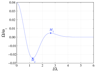
Figure 1: The acquired controlled phase per unit time $\Omega$, as a function of distance $l$. The maximal value is at $M_{2}$ where $l/\lambda=1.25$; a time of $128/\omega_{1}$ is required to obtain a control-phase of value $\pi$.

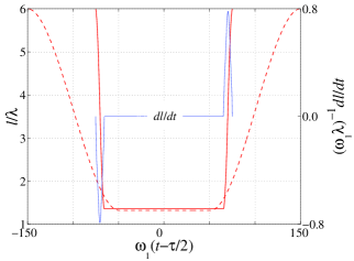
Figure 2: The optimal path $l(t)$ obtained after optimization for an adiabatic (dashed curve) and fast-approach (solid curve) gate ($\dot{l}$ also plotted for fast-approach).

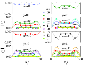
Figure 3: Absolute values of the coefficients $f_{mn}^{ij}(t)$ (Eq.(9)) for the optimal adiabatic gate. The upper indexes represent the four initial condition $f_{mn}^{ij}(0)=\delta_{im}\delta_{jn}$, $0\leq i,j\leq 1$. To a good approximation, eigenstates are self-evolved at all times, as expected in adiabatic evolution.

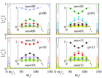
Figure 4: Absolute values of the coefficients $f_{mn}^{ij}(t)$, as in Fig. 3, for the fast-approach gate. Eigenstates in $W$ are restored at the end of each fast step.

We first applied the optimization procedure to an adiabatic gate. Good fidelity is expected in an adiabatic evolution. However, propagating adiabatically, one has an error of the order of $\dot{l}$. Using the optimization scheme, the gate was improved and the error reduced. For the initial $l$ trial function we took $l_{p}=l_{\rm M}=1.25\lambda$, and $\tau=300/\omega_{1}$, $t_{1}=\tau-t_{2}=100/\omega_{1}$, $q=0$. This choice was constrained by the requirement that the evolution be adiabatic, i.e., that $|\dot{l}M|\ll 1$. We expect some phase to be acquired outside the plateau, so we took the plateau time to be smaller than $\pi/|\Omega_{\rm{}_{M}}|\approx 128/\omega_{1}$. The maximal value of $|\dot{l}|$ is $\approx 0.07{\lambda}/{\omega_{1}}$, consistent with adiabaticity. The optimized parameters are $l_{p}^{\rm opt}=1.32\lambda=1.06l_{\rm M}$, $t_{1}^{\rm opt}=100.47\omega_{1}$, $t_{2}^{\rm opt}=200.94\omega_{1}$. The optimized $l$ is shown in Fig. 2. We ended the optimization with $J=0.00003$, $F=0.99999$, and $D=0.99999$. Parameter variations of the order of $10\%$ affect $D$ and $F$ to about one part in $10^{5}$, while the acquired phase (here $\phi=3.1416$) is very sensitive to any change in $l$, in particular ${\delta\phi}/{\phi}\approx(\delta t_{2}-\delta t_{1})/(t_{2}-t_{1})$, since $\phi\approx\Omega(l_{p})(t_{2}-t_{1})$. The coefficients of the evolved computational basis are shown in Fig. 3.

The fast-approach gate is considered next. We expect the optimal path for this scheme to be obtained when at the end of each fast step (approach or departure) all eigenstates in $W$ are restored to themselves while the required phase difference is obtained at the plateau. To select a trial function we therefore choose $(t_{2}-t_{1})=128/\omega_{1}$, $l_{\rm M}=1.25\lambda$, $t_{1}=11/\omega_{1}$, $\tau=150/\omega_{1}$. This gives non-adiabatic evolution, $\mbox{max}(|\dot{l}|)\approx 0.64\,\lambda/\omega_{1}$. The optimized $l$ is the solid curve of Fig. 2. The optimized parameters are $l_{p}^{opt}=1.36\,\lambda$, $t_{1}^{opt}=9.38\,\omega_{1}$, $t_{2}^{opt}=140.49\,\omega_{1}$, $\tau^{opt}=150.22\,\omega_{1}$. Optimization iterations were stopped when $J=0.006$, $D=0.997$, $F=0.999$, and $\phi=3.14$. The accuracy for $F$ and $D$ is maintained as long as parameters for $l$ are $\approx 1\%$ from the optimized values. With such variations, the accuracy for $\phi$ is $\approx 0.01$. Varying the plateau time linearly from $0$ to $t_{2}^{opt}-t_{1}^{opt}$ while keeping the approach and departure shapes fixed, produces a linear curve for $\phi(t)$ with slope $\Omega(l_{p})=0.0237\omega_{1}$ with standard-deviation $\approx 10^{-4}$. With this set of plateau times the fidelity measures demonstrate oscillatory behavior about their optimized values with deviations of about $10^{-3}$. The coefficients of the evolved computational basis are shown in Fig. 4. Initial temporal eigenstates were recovered at the plateau. The approach and departure times are reduced by a factor of $10$, leakage outside the computational basis is restricted to less than 0.1%, while excellent agreement with an ideal P$(\pi)$ gate is maintained.

VI A Further Application of the Fast-Approach Procedure

The fast-approach scheme suggested by our analysis is essentially model independent. For example, let us briefly consider the implementation of such a fast-approach scheme for high-fidelity transport in the experimental system of Refs. Bloch where the computational basis was taken to be the hyperfine states of ⁸⁷Rb atoms trapped in an optical lattice in the Mott insulating regime. The effective potentials experienced by the atoms depended on their internal hyperfine states and the laser polarization. The gate was not implemented adiabatically. For approach distances of half a lattice spacing and approach times, $\tau$, longer than $\sim 2\pi/\omega$, where $\omega$ is the harmonic frequency at the minimum of the optical lattice, the degree of infidelity obtained was $\sim 5\%$. In a preliminary study, we applied optimal control to the approach step of this gate. The spatial wave packet of the atoms $\phi(x-R(t),t)$ can be evolved upon moving the trap minima via a path $l(t)$ such that $(\ddot{R}-\ddot{l})+\omega^{2}(R-l)=-\ddot{l}$, and the probability to escape the ground state at time $t$ is given by $P(t)=1-|\langle\phi(x-l(t),t)|\phi(x-R(t),t)\rangle|^{2}=1-e^{(-y^{2}(t)/4\lambda^{2})}$, where $R(t)$ is the center of the wave packet and $y(t)\equiv R(t)-l(t)$ with initial condition $y(0)=0$ Japha . Taking $\sqrt{y^{2}(\tau)+\dot{y}^{2}(\tau)}$ as the objective, we were able to find a smooth path $l(t)$ that reduces the approach time by 65%, with $y^{2}(\tau)<<10^{-12}$ so that losses were reduced from several percent to $P(\tau)\approx 2y(\tau)^{2}/4\lambda^{2}\approx 10^{-12}$. More work is planned to minimize the run time, and implement the complete gate, including the time interval of interaction, yet clearly our scheme is able to significantly increase fidelity while somewhat reducing the required time for the approach.

VII Conclusion

In summary, using optimal-control, we improved the adiabatic phase gate, designed a new fast-approach phase gate, and demonstrated the new fast-approach scheme for a simple model and a recent experiment. More sophisticated models with additional degrees of freedom could further exploit optimal-control techniques.

A few last remarks are in order. The 1D model considered here is obtained in reality from a physical 3D trap assuming that the ground state of the transverse degrees of freedom is maintained through the process. A 3D model, where the moving potential remains 1D, yet transverse excitations are allowed, could be better for designing a fast gate. In addition, for any scheme to be practical, it is essential that the accuracy of the gate depend weakly on small changes in $l$. Here we saw that different fidelity measures are quite robust, while the phase is very sensitive to changes in $l$. As a result the gates can be easily adjusted to give a P$(\phi)$ gate with any $\phi$ by changing the time duration of the plateau. In practice, feedback learning techniques may be used to assure stability and to adjust the phase. Finally, for a complete scheme of computation, one also needs single qubit gates. This is another point at which degeneracy causes problems, as the computational basis of the two oscillators needs to be un-entangled. While these points deserve further study, they were disregarded here, as our main focus was that one could use optimal-control techniques and a fast-approach scheme for the implementation of the control-phase gate in models of cold atoms in an optical lattice, significantly reducing the gates time while maintaining high fidelity.

Acknowledgments This research was supported by the Israel Science Foundation (Grant Nos. 11-02 and 8006/03), U.S.-Israel Binational Science Foundation (No. 2002147), and James Franck Program (German-Israel) in Laser-Matter Interactions. We are grateful to David Tannor and Ehoud Pazy for useful discussions.

Appendix A Entanglement power of the CP$(\phi)$ gate

An important property of the CP$(\phi)$ gate (and hence of any P$(\phi)$ gate) is that the phase $\phi$ can be used to measure the entanglement power of the gate. To see this consider a general two qubit state $|\Psi\rangle=\sum_{m,n=0}^{1}a_{mn}|m,n\rangle$. The action of CP$(\phi)$ on this state is,

$$A\equiv\begin{pmatrix}a_{00}&a_{01}\cr a_{10}&a_{11}\end{pmatrix}~{}\longrightarrow~{}\tilde{A}=\begin{pmatrix}a_{00}&a_{01}\cr a_{10}&\sigma a_{11}\end{pmatrix}$$ (15)

where $\sigma=\exp({i\phi})$. Generally, if $\rho$ is the reduced density matrix of a bipartite pure system, the usual entanglement measures of $\rho$ are given by the purity (linear entanglement) measure $M_{1}\equiv-{\rm Tr}{\rho^{2}}$, or the Von Neumann entropy $M_{2}\equiv-\,{\rm Tr}\,\rho\log_{2}\rho$. There are important mathematical features of interest when one chooses a measure, such as convexity. Here we are only interested in a measure of the degree of entanglement. The reduced density matrix of two qubits can be written as

$$\rho=p{\cal P}+(1-p)(I-{\cal P})\,,$$ (16)

where $0\leq p\leq 1$, ${\cal P}$ is the one dimensional projection onto the $p$ eigenstate of $\rho$, and $I$ is the identity in the two level system sub-space. For such a state

$$M_{1}=-[p^{2}+(1-p)^{2}]\,,$$ (17)

$$M_{2}=-p\log_{2}p-(1-p)\log_{2}(1-p)\,.$$ (18)

The line ordering imposed by these measures is the same line ordering obtained from the determinant of the reduced density matrix: $\det(\rho)=p(p-1)$. We therefore use the change in this determinant as a measure for the entanglement induced by the gate:

$$\Delta(\Psi;\phi) \equiv \mbox{det}(\tilde{A}\tilde{A}^{\dagger})-\mbox{det}(AA^{\dagger})$$ (19)

$$= 2\Re\left(a_{00}\,a_{11}\,\bar{a}_{10}\,\bar{a}_{01}\,(1-\sigma)\right)$$ (20)

$$= 4\Re\left(-i~{}r\exp\left({i(\gamma+\frac{\phi}{2})}\right)\,\sin(\frac{\phi}{2})\right)\,,$$ (21)

where $r\exp({i\gamma})\equiv a_{00}\,a_{11}\,\bar{a}_{10}\,\bar{a}_{01}$. The maximal change is obtained when $r$ and $\sin(\gamma+{\phi}/{2})$ are maximal, i.e., when $|a_{mn}|={1}/{2}$ and $\gamma=({\pi-\phi})/{2}$. The entangling power of the CP$(\phi)$ gate and hence of any P$(\phi)$ gate is

$$\mbox{max}_{\Psi}(\Delta(\Psi,\phi))=\frac{1}{4}\sin(\frac{\phi}{2})\,.$$ (22)

Maximum entanglement power is obtained for $\phi=\pi$ (also for the CN gate).

Appendix B Asymmetric double-well

Two counter-propagating laser beams at a fundamental frequency and at its second harmonic, with wave numbers $k$ and $2k$, and intensities, produce an effective standing wave optical potential of the form

$$V(k,x)=V_{0}[\cos^{2}(kx+\delta)+\alpha\cos^{2}(2kx)],$$ (23)

where $V_{0}$ is proportional to the intensity of the fundamental, $\alpha$ is determined by beam intensities and detuning ratios, and $\delta$ is determined by the relative phase between the fundamental and second harmonic. The wave number $k$ can be tuned by manipulating the angle between the right and left laser beams. The effective potential thus formed is an array of double wells, with $\alpha$ determining the relative heights of the well minima. For $\delta>0$, the wells are non-symmetric. Let $x_{1}(k)$, $x_{2}(k)$ denote the positions of the minima of a specific double well, where $x_{1}(k)<x_{2}(k)$. The greater $\delta$, the larger $V(x_{2}(k))$ relative to $V(x_{1}(k))$, as well as $V^{\prime\prime}(x_{2}(k))$ relative to $V^{\prime\prime}(x_{1}(k))$. One can add a linear potential of the form

$$\tilde{V}(x,k)=-A(k)x$$ (24)

to $V(k,x)$ so the resulting potential, $V_{\rm{eff}}$, will have equal well minima, $V_{\rm{eff}}(x_{2}(k))=V_{\rm{eff}}(x_{1}(k))$. This requires

$$A(k):=V_{0}\frac{V(x_{2}(k))-V(x_{1}(k))}{x_{2}(k)-x_{1}(k)}\,.$$ (25)

As a result of the additional linear potential, there is an increase in the ratio of the second derivatives at the well minima of $V_{\rm{eff}}$. Note that the original potential $V(k,x)$ is a function of $kx$, $V(k,x)=f(kx)$, thus

$$V(k^{\prime},x) = f(k\frac{k^{\prime}}{k}x)=V(k,\frac{k^{\prime}}{k}x)\,,$$ (26)

$$k^{\prime}x_{i}(k^{\prime}) = kx_{i}(k)\,,$$ (27)

and hence

$$\frac{A(k^{\prime})}{k^{\prime}} = \frac{V(k^{\prime},x_{2}(k^{\prime}))-V(k^{\prime},x_{1}(k^{\prime}))}{k^{\prime}\left(x_{2}(k^{\prime})-x_{1}(k^{\prime})\right)}\,,$$ (28)

$$= \frac{V(k,x_{2}(k))-V(k,x_{1}(k))}{k\left(x_{2}(k)-x_{1}(k)\right)}$$ (29)

$$= \frac{A(k)}{k}\,.$$ (30)

$A(k)/k$ is independent of $k$ and (24) can be written as

$$\tilde{V}(k^{\prime},x)=-V_{0}Ck^{\prime}x$$ (31)

where $C$ is a constant that may be determined by (25) for any $k$. Thus,

$$V_{\rm{eff}}(k,x)=V_{0}[\cos^{2}(kx+\delta)+\alpha\cos^{2}(2kx)-Ckx]\,,$$ (32)

is a function of $kx$. For such a potential, variations of $k$ scale $x$. The distance $l(k)$ between the two minima in a double well is thus a parameter scaled by $k$, $l(k^{\prime})={k^{\prime}\over k}l(k)$, while keeping the values of potential values at minimal points unaltered as well as the ratios of second derivatives at the minima. To maintain the values of second derivatives at the minimum constant as one varies $k$, one can modify the laser intensities to depend on $k$ such that

$$V_{0}\rightarrow V_{0}(k):=\frac{V}{k^{2}}\,.$$ (33)

References

- (1) D. Jaksch, C. Bruder, J. I. Cirac, C. W. Gardiner, and P. Zoller, Phys. Rev. Lett. 81, 3108-3111 (1998).
- (2) I.H. Deutsch, P.S. Jessen, Phys. Rev. A57, 1972 (1998).
- (3) G.K. Brennen, C.M. Caves, P.S. Jessen, and I.H. Deutsch, Phys. Rev. Lett. 82, 1060 (1999).
- (4) D. Jaksch, H.-J. Briegel, J. I. Cirac, C. W. Gardiner, and P. Zoller, Phys. Rev. Lett. 82, 1975 (1999).
- (5) T. Calarco, E. A. Hinds, D. Jaksch, J. Schmiedmayer, J. I. Cirac, and P. Zoller, Phys. Rev. A61 022304 (2000).
- (6) E. Charron, E. Tiesinga, Frederick Mies, and C. Williams, Phys. Rev. Lett. 88, 077901 (2002).
- (7) J.K. Pachos and P.L. Knight, Phys. Rev. Lett. 91, 107902 (2003).
- (8) K. Eckert, J. Mompart, X. X. Yi, J. Schliemann, D. Bruss, G. Birkl, and M. Lewenstein, Phys. Rev. A66, 042317 (2002).
- (9) R. Dumke, M. Volk, T. Müther, F. B. J. Buchkremer, G. Birkl, and W. Ertmer, Phys. Rev. Lett. 89, 097903 (2002).
- (10) L. Guidoni and P. Verkerk, J. Opt. B1, R23 (1999).
- (11) O. Mandel, M. Greiner, A. Widera, T. Rom, T. W. Hänsch and I. Bloch, Nature (London) 425, 937 (2003); Bloch, Phys. Rev. Lett. 91, 010407 (2003).
- (12) D. Jaksch, J. I. Cirac, and P. Zoller, S. L. Rolston, R. Côté and M. D. Lukin, Phys. Rev. Lett. 85, 2208 (2000).
- (13) J.I. Cirac, P. Zoller, Physics Today 57, 38, March 2004.
- (14) For an extension of optimal control, see S.E. Sklarz and D. J. Tannor, Phys. Rev. A66, 053619 (2002).
- (15) D. Deutsch, Proc. R. Soc. A400, 97 (1985).
- (16) J.P. Palao and R. Kosloff, Phys. Rev. Lett. 89, 188301 (2002); Phys. Rev. A68, 062308 (2003).
- (17) Y. Japha and Y. B. Band, J. Phys. B35, 2383 (2002).