Mutual information–based approach to adaptive homodyne detection
of quantum optical states

Abstract

I propose an approach to adaptive homodyne detection of digitally modulated quantum optical pulses in which the phase of the local oscillator is chosen to maximize the average information gain, i.e., the mutual information, at each step of the measurement. I study the properties of this adaptive detection scheme by considering the problem of classical information content of ensembles of coherent states. Using simulations of quantum trajectories and visualizations of corresponding measurement operators, I show that the proposed measurement scheme adapts itself to the features of each ensemble. For all considered ensembles of coherent states, it consistently outperforms heterodyne detection and Wiseman’s adaptive scheme for phase measurements [H.M. Wiseman, Phys. Rev. Lett. 75, 4587 (1995)].

I Introduction

Digital communication with modulated optical pulses is essential to the modern interconnected world. While most optical communication schemes use strong electromagnetic signals that are well described classically textbook , some electromagnetic signals can exhibit manifestly non-classical behavior and need to be analyzed using quantum mechanics wolf . The latter situation arises, for example, when electromagnetic signals are extremely weak either by design, as in quantum cryptography crypt , or out of necessity, as in deep space communications space .

Among the many types of quantum states of electromagnetic field that can be used for communication are photon number states, coherent states, and quadrature-squeezed states wolf . Coherent states are especially popular because they are quasiclassical in their properties and relatively easy to prepare. There are also many different ways to measure electromagnetic states, with direct photon counting, heterodyne detection, and homodyne detection being easiest to implement in experiment. However, because of quantum uncertainty, none of these methods can perfectly measure both quadratures of the field. In fact, one can only decrease the measurement error in one quadrature at the expense of an increase in the other wolf ; cavesRMP . In heterodyne detection, the quickly rotating phase of the local oscillator implies that all quadratures are measured equally well, which makes this scheme the most versatile. Homodyne detection is the other extreme: It keeps the local oscillator phase constant and therefore measures one quadrature perfectly, while providing no information whatsoever about the perpendicular one.

In this paper, I consider quantum detection of coherent states using homodyne detection with the adaptively changing phase of the local oscillator f1 . Allowing adaptive phase in homodyne measurements significantly expands the set of possible quantum measurement of optical pulses, while its experimental realization remains relatively straightforward. This type of quantum measurement was proposed recently by Wiseman for various phase measurement problems and was demonstrated to be superior to other types of measurements both theoretically [see, for example, Ref. wiseman05 and references therein] and experimentally hideoexp .

There are many criteria for choosing a quantum measurement among different alternatives. For example, one can try to minimize the probability of error in determining the source variable from measurement results QAM ; geremia , the average squared deviation of the best estimate from the actual value of the source variable wiseman95 , or maximize the mutual information between the source variable and the measurement results QAM ; cavesRMP . Optimization of these target functions is interrelated to some extent osaki98 ; for example, zero probability of error or zero deviation of the estimate implies maximum mutual information and vice versa. However, in this paper, I focus on maximizing the mutual information because it is the mutual information that defines the information capacity of a communication channel textbook ; preskill .

Note that, for quantum channels, one can define different types of classical information capacities depending on whether one can perform collective quantum measurements or only measure one state at a time, and whether communication is allowed between measurement shor04 . While collective measurements potentially result in a higher capacity, they highly impractical in the case of continuous communication with coherent optical pulses. Performing adaptive measurements of individual pulses is therefore an attractive way to extract more information from a given state without resorting to advanced quantum measurement techniques.

II Theory

Let the state of the electromagnetic field be given by a coherent state $\mathop{\left|\alpha_{k}\right\rangle}\nolimits$ that depends on the value of the source variable $k$. I will assume for simplicity that the source variable can only take a finite number of values with known a priori probabilities $p_{k}$. These probabilities and states form an ensemble ${\cal E}=\left\{p_{k},\mathop{\left|\alpha_{k}\right\rangle}\nolimits\right\}$, which appears in the problem of the classical information content of quantum states preskill . For efficient communication, one needs to maximize the mutual information between the source variable and the measurement results by optimizing the quantum measurement procedure. In general, this problem is not solved, although optimal solutions are known for certain symmetric ensembles of states symmetric , and a “pretty good”, but not necessarily optimal, measurement can be derived for any ensemble pgm ; QAM . In this paper, I consider only those measurements that can be realized using balanced photodetection with an arbitrary time dependence of the local oscillator phase. To the best of my knowledge, the optimal solution is not known in this case either.

Figure 1 shows the relevant experimental setup, similar to the one used recently to demonstrate improved optical phase estimation with adaptive homodyne measurements hideoexp . The optical cavity supports a mode whose state is described by one of the wave functions from the ensemble ${\cal E}$ above. One of the mirrors of the otherwise lossless cavity is not perfect, so the radiation leaks out and mixes with the strong beam of the local oscillator (LO) at the 50-50 beam splitter (BS). In balanced photodetection, one records the difference between the photocurrents of the two detectors (P1,P2) in order to reduce the strong background due to the local oscillator. The photocurrent record is then analyzed by the signal processor (SP) to determine the optimal phase $\varphi$ of the local oscillator (LO) for subsequent measurement. The phase can be updated continuously or, more practically, discretely with a small time step $\Delta t$. I will assume that there are no time delays in the feedback loop.

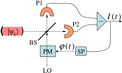
Figure 1: Schematic of adaptive homodyne measurement. The signal processor (SP) analyzes the collected photocurrent record $\{I(\tau):\,0<\tau<t\}$ and adjusts the phase of local oscillator (LO) using the phase modulator (PM).

During a detection time interval $(t,t+\Delta t)$, each of photodetectors P1 and P2 generates a certain amount of electronic charge. In the following, I will assume that the photodetectors are noiseless and perfectly efficient. If the cavity state is initially given by a coherent state $\mathop{\left|\alpha_{k}\right\rangle}\nolimits$ with the complex amplitude $\alpha_{k}$, and the approximation of a strong local oscillator applies, the difference between the generated charges can be normalized to give wiseman95

$$\Delta Q(t)=\int_{t}^{t+\Delta t}I(\tau)d\tau\approx 2e^{-t/2}\Re[\alpha e^{-i\varphi(t)}]\Delta t+dW,$$ (1)

where $\Re$ represents the real part of a number, $dW$ is the Wiener increment of the quantum photodetection noise, satisfying $\left<dW^{2}\right>=\Delta t$, and time has been scaled by the cavity decay time. The factor $e^{-t/2}$ in Eq. (1) describes amplitude decay of any coherent state in the cavity due to leakage through the imperfect mirror. Each coherent state of the field in the cavity therefore produces exponentially shaped pulses of photocurrents starting at time $t=0$.

The probability distribution function for the accumulated photocharge is given by wiseman97

$$P\left(\Delta Q(t)\right)={\cal N}\left(\Delta Q(t);2\Delta t\Re[\alpha e^{-t/2-i\varphi(t)}],\Delta t\right),$$ (2)

where ${\cal N}\left(\Delta Q(t);A,\sigma^{2}\right)\equiv\frac{1}{\sqrt{2\pi}\sigma}e^{-\frac{(\Delta Q(t)-A)^{2}}{2\sigma^{2}}}$ is the Gaussian distribution with the mean $A$ and standard deviation $\sigma$. For any measured value of the photocharge $\Delta Q(t)$, one can update the prior probabilities of the source variable using Bayes’ rule:

$$p_{k}(t+\Delta t)=\frac{p_{k}(t){\cal N}\left(\Delta Q(t);2\Delta t\Re[\alpha_{k}e^{-t/2-i\varphi(t)}],\Delta t\right)}{\sum_{k}p_{k}(t){\cal N}\left(\Delta Q(t);2\Delta t\Re[\alpha_{k}e^{-t/2-i\varphi(t)}],\Delta t\right)}.$$ (3)

For each result of the current measurement step, we therefore learn something about the source variable. The gain in information (reduction in uncertainty) about the source variable $k$ is given by

$${\cal G}\,[\Delta Q(t)]=H(\left\{p_{k}(t)\right\})-H(\left\{p_{k}(t+\Delta t)\right\}),$$ (4)

where $H(\left\{p_{k}\right\})=-\sum_{k}p_{k}\log_{2}p_{k}$ is the Shannon entropy of a probability distribution textbook ; preskill . The mutual information between the measurement result $\Delta Q(t)$ and the source variable is simply the information gain (4) averaged over the random outcomes $\Delta Q(t)$:

$${\cal I}\,[\Delta Q(t):k]=\left<H(\left\{p_{k}(t)\right\})-H(\left\{p_{k}(t+\Delta t)\right\})\right>_{\Delta Q(t)}.$$ (5)

If the time period $\Delta t$ is sufficiently small, the standard deviation of the photocharge probability distribution becomes much larger than its mean, $\sigma\gg A$, because in Eq. (2), the mean scales as $\Delta t$, whereas the standard deviation scales as $\sqrt{\Delta t}$ f2 . In this case, the photocharge accumulated during one sampling period carries very little information about the source variable, and only the totality of the sampled photocharges may be sufficient to distinguish the states $\mathop{\left|\alpha_{k}\right\rangle}\nolimits$. Below I will consider only this situation because it arises naturally in adaptive measurements.

The Gaussian distributions (2), all having the same dispersion, are then very wide and only slightly shifted from the zero mean. Expanding the exponentials in $A$ up to the first order, we obtain

$${\cal N}\left(\Delta Q;A,\sigma^{2}\right)\approx\frac{1}{\sqrt{2\pi}\sigma}e^{-\frac{\Delta Q^{2}}{2\sigma^{2}}+\frac{\Delta Q}{\sigma^{2}}A}$$ (6)

$$\approx{\cal N}\left(\Delta Q;0,\sigma^{2}\right)\left(1+\frac{\Delta Q}{\sigma^{2}}A\right).$$ (7)

The mutual information (5) is then approximately given by

$$\begin{array}[]{l}{\cal I}\,[\Delta Q(t):k]\approx\left<p_{k}{\cal N}\left(\Delta Q(t);0,\Delta t\right)\left(1+\frac{\Delta Q(t)}{\Delta t}A_{k}(t)\right)\times\right.\\ \left.\times\log\left(\frac{1+\frac{\Delta Q(t)}{\Delta t}A_{k}(t)}{\sum_{l}p_{l}\left[1+\frac{\Delta Q(t)}{\Delta t}A_{l}(t)\right]}\right)\right>_{k,\Delta Q}\approx\frac{\left<A(t)^{2}\right>-\left<A(t)\right>^{2}}{2\Delta t},\end{array}$$ (8)

where in our case $A_{k}(t)=2e^{-t/2}\Re[\alpha_{k}e^{-i\varphi(t)}]\Delta t$, $\left<A(t)\right>=\sum_{k}p_{k}(t)A_{k}(t)$, and $\left<A(t)^{2}\right>=\sum_{k}p_{k}(t)A_{k}^{2}(t)$.

Introducing new notation $X_{k}=\Re(\alpha_{k})$ and $Y_{k}=\Im(\alpha_{k})$, where $\Im(.)$ is the imaginary part of a complex number, it is easy to show that the last term in Eq. (8) is proportional to

$$\begin{array}[]{l}2\sigma^{2}_{X}(t)\cos^{2}\varphi+2\sigma^{2}_{Y}(t)\sin^{2}\varphi+4\sigma_{XY}(t)\sin\varphi\cos\varphi=\\ \sigma^{2}_{X}(t)+\sigma^{2}_{Y}(t)+(\sigma^{2}_{X}(t)-\sigma^{2}_{Y}(t))\cos 2\varphi+2\sigma_{XY}(t)\sin 2\varphi,\end{array}$$ (9)

where $\sigma^{2}_{X}(t)\equiv\sum_{k}p_{k}(t)X_{k}^{2}-\left(\sum p_{k}(t)X_{k}\right)^{2}$, $\sigma^{2}_{Y}(t)\equiv\sum_{k}p_{k}(t)Y_{k}^{2}-\left(\sum p_{k}(t)Y_{k}\right)^{2}$, and $\sigma_{XY}\equiv\sum_{k}p_{k}(t)X_{k}Y_{k}-\left(\sum p_{k}(t)X_{k}\right)\left(\sum p_{k}(t)Y_{k}\right)$. Equation (9) is maximized when

$$\varphi(t)=\frac{1}{2}{\rm Arg}\left[(\sigma^{2}_{X}(t)-\sigma^{2}_{Y}(t))+2i\sigma_{XY}(t)\right],$$ (10)

where ${\rm Arg}[.]$ is the argument of a complex number.

Note that Eq. (8) provides a simple geometrical interpretation of the considered maximization problem. The ensemble $\{p_{k},\mathop{\left|\alpha_{k}\}\right\rangle}\nolimits$ defines an ensemble of points $\{p_{k},X_{k},Y_{k}\}$ in the phase space $XOY$. These points can be projected onto a new coordinate axis $OP$, which forms an angle $\varphi$ with axis $OX$, to produce a new ensemble $\{p_{k},P_{k}\}$. The dispersion of this ensemble $\{p_{k},P_{k}\}$ is then proportional to the expression (8). In our maximization of mutual information, we are therefore looking for a configuration that maximizes the expected dispersion of the measured field quadrature at each measurement step.

The measurement scheme given by Eq. (10) is adaptive because the probabilities $p_{k}(t)$ are updated according to Eqs. (3) after each measurement step. The resulting detection scheme is locally optimal in the sense that the average information gain is maximized at each measurement step. For convenience, I will call this adaptive scheme LMMI measurement, from Local Maximization of Mutual Information. Note that, even though local optimization can sometimes lead to a globally optimal solution, it is not a general rule and there is no guarantee that the LMMI measurement is optimal globally, i.e., it maximizes the information gain from the entire measurement record. However, I demonstrate below that the LMMI measurement is quite versatile and, in all considered examples, performs better than heterodyne detection and Wiseman’s adaptive scheme for phase measurements.

Before presenting the results of numerical quantum trajectory simulations, it is useful to review some limits on the information capacity of optical communication channels cavesRMP . For example, if one uses an ensemble of coherent states and (nonadaptive) heterodyne detection, the mutual information for a single pulse has an upper bound ${\cal I}_{1}=\log_{2}\left(1+\left<n\right>\right)$ bits, where $\left<n\right>\equiv\sum_{k}p_{k}|\alpha_{k}|^{2}$ is the average number of photons, i.e., the energy used per pulse. This bound can be saturated using an infinite ensemble of coherent states with the Gaussian distribution of prior probabilities. If one allows squeezed states and homodyne detection, the upper bound increases to ${\cal I}_{2}=\log_{2}(1+2\left<n\right>)$. Presumably, this is the best one can do with non-adaptive balanced photodetection, but the fragility of squeezed states makes this bound difficult to reach in practice. Finally, another bound on the mutual information is provided by the Holevo information of the given ensemble of pure states $\chi({\cal E})=-{\rm Tr\,}{\hat{\rho}\log_{2}\hat{\rho}}$, where $\hat{\rho}=\sum_{k}p_{k}\mathop{\left|\alpha_{k}\right\rangle}\nolimits\mathop{\left\langle\alpha_{k}\right|}\nolimits$ preskill ; cavesRMP . The Holevo information itself has a upper bound of ${\cal I}_{3}=\log_{2}(1+\left<n\right>)+\left<n\right>\log_{2}(1+1/\left<n\right>)$. This maximum capacity can be achieved using ensembles consisting of photon number states with the Boltzmann distribution of prior probabilities and using perfect photon counting for detection cavesRMP . However, controlled production of photon number states and perfect photon counting remain technically challenging and are unlikely to become practical in the nearest future.

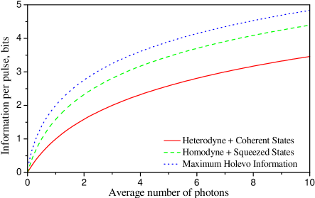
Figure 2: Some general limits on the information capacity of bosonic communication channels.

Figure 2 shows all these bounds on a single graph. Note that for strong signals, $\left<n\right>\gg 1$, these bounds are approximately given by ${\cal I}_{1}\approx\log_{2}\left<n\right>$, ${\cal I}_{2}\approx\log_{2}\left<n\right>+1$, and ${\cal I}_{2}\approx\log_{2}\left<n\right>+\log_{2}e\approx\log_{2}\left<n\right>+1.443$. Therefore, in this semiclassical regime, the difference between the best performance of heterodyne detection, ${\cal I}_{1}$, and the performance of the best possible quantum measurement scheme, ${\cal I}_{3}$, is relatively small, which probably explains the popularity of heterodyne detection in practical applications. It is only in the limit of small photon numbers that one may noticeably improve upon heterodyne detection with an adaptive measurement scheme. Note also that the best energy efficiency of communication, i.e., the amount of information transmitted per number of photons used, is achieved with small-photon-number ensembles as well cavesRMP .

III Numerical simulations

To illustrate the performance of the proposed adaptive measurement scheme, I have performed numerical quantum-trajectory simulations plenio ; wiseman_repres for three different ensembles of relatively weak coherent states with $\left<n\right><5$. Figures 3(a)–5(a) show these three ensembles on the $XOY$ phase plane, with the centers of circles $(X_{k},Y_{k})$ representing the amplitudes of the corresponding states of the ensemble and the radius of each circle representing the intrinsic quantum uncertainty of a coherent state wolf ; cavesRMP .

The first ensemble (Fig. 3(a)) consists of eight equiprobable states with the same amplitude $|\alpha_{k}|=\sqrt{2}$ and evenly distributed phases. In communications language textbook , this modulation scheme is known as phase-shift keying (PSK), and the ensemble is called 8PSK for short. The second ensemble (Fig. 4(a)) consists of 16 equiprobable states with the real and imaginary parts of their amplitudes ranging from -1.5 to 1.5 with unit increment. This is so-called quadrature-amplitude modulation (QAM) and the ensemble is called 16QAM. The third ensemble (Fig. 5(a)) consists of 10 equiprobable states arranged in the shape of a three-lobe star, with all states having integer amplitudes from 0 to 3 and phases of $0,\,2\pi/3,$ or $4\pi/3$. This type of combined phase and amplitude modulation is not usually used in communications but illustrates well some properties of the proposed adaptive measurement scheme. For convenience, I will call it STAR.

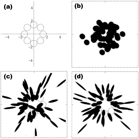
Figure 3: (a) Phase space representation of the ensemble of eight equiprobable coherent states $\mathop{\left|\alpha_{k}\right\rangle}\nolimits=\mathop{\left|\sqrt{2}e^{2\pi ik/8}\right\rangle}\nolimits,\,k=1..8$, with the same amplitude and evenly distributed phases (8PSK). (b)-(d) The original ensemble and visualization of 50 projector operators that represent POVM’s corresponding to (b) (nonadaptive) heterodyne measurement, (c) Wiseman’s adaptive phase measurement, and (d) LMMI measurement.

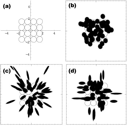
Figure 4: Same as Fig. 3 for an equiprobable quadrature-amplitude modulated ensemble of 16 coherent states (16QAM).

The numerical simulations were performed using Mathematica software. The discrete time step was $\Delta t=5\times 10^{-3}$, so that $\alpha\Delta t\ll\sqrt{\Delta t}$ for all simulates states. Each quantum trajectory was simulated from $t=0$ to $t=10$, by which point the residual photon population of the cavity is $e^{-10}<5\times 10^{-5}$ of the initial value, and the information still extractable from it is negligible. For each ensemble, I simulated a total of 10000 trajectories, randomly choosing an initial coherent state from the given ensemble with the respective a priori probabilities and recording the total information gain ${\cal G}$ for each trajectory. The statistic mean of the information gain and its standard deviation were estimated from these data. They are presented for each ensemble in Table 1 in the form of the $2\sigma$-confidence intervals for the mutual information between the source variable $k$ and the entire photocharge record $\{\Delta Q(t):0<t<10\}$. The table also lists the average number of photons per pulse for each ensemble $\left<n\right>$, the optimal mutual information of heterodyne detection for this number of photons ${\cal I}_{1}(\left<n\right>)$, and the Holevo information $\chi(\cal E)$ of each ensemble. The latter was calculated by truncating the Hilbert space to the maximum photon number of 100.

To provide benchmarks for the performance of the LMMI measurement, I have also simulated quantum trajectories for a discrete approximation to heterodyne detection, in which the phase of the local oscillator is increased by 0.1 rad after each measurement step, and Wiseman’s original adaptive phase measurement scheme, in which the local oscillator phase is changed by $\Delta Q(t)/\sqrt{t}$ after each measurement step wiseman95 . Note that Wiseman’s scheme was originally proposed to measure a continuously and uniformly distributed random phase, and therefore may be ill-suited to the problem of classical information extraction, especially for ensembles 16QAM and STAR. However, Wiseman’s scheme is the only adaptive homodyne detection scheme widely discussed in the literature, and it is therefore instructive to compare its properties to those of the adaptive LMMI measurement. Table 1 lists the estimated mutual information for all combinations of the three considered detection techniques and the three ensembles. I will defer the discussion of these results to the following sections.

Ensemble ${\cal E}$	8PSK	16QAM	STAR
$\left<n\right>$	2	2.5	4.2
${\cal I}_{1}(\left<n\right>)$, bits	1.585	1.807	2.379
$\chi({\cal E})$, bits	2.449	2.859	2.751
${\cal I}_{het}({\cal E})$, bits	$1.492\pm 0.008$	$1.743\pm 0.011$	$1.872\pm 0.009$
${\cal I}_{W}({\cal E})$, bits	$1.676\pm 0.006$	$1.771\pm 0.008$	$1.649\pm 0.005$
${\cal I}_{LMMI}({\cal E})$, bits	$1.692\pm 0.005$	$1.805\pm 0.011$	$2.206\pm 0.007$

Table 1: Some properties of the considered ensembles and results of numerical simulations for the average information gain (mutual information) using heterodyne detection ${\cal I}_{het}({\cal E})$, Wiseman’s adaptive phase measurement ${\cal I}_{W}({\cal E})$, and adaptive LMMI measurement ${\cal I}_{LMMI}({\cal E})$.

IV POVM visualizations

Adaptive or not, any quantum measurement with a predetermined algorithm for choosing the local oscillator phase can be represented as a generalized quantum measurement known as the positive operator-valued measure (POVM) preskill ; wiseman_repres . Wiseman has shown wiseman_repres that, for measurements with any time dependence of the local oscillator phase, these POVMs consist of an infinite number of projectors onto pure squeezed states $\mathop{\left|\alpha,\xi\right\rangle}\nolimits$. To get additional insight in the properties of such measurements, it is helpful to visualize a sample of these squeezed states on the $XOY$ plane as ellipses that represent the density plot of the Wigner functions of these states. Each ellipse corresponds to one quantum trajectory (the outcome of one complete measurement) according to the equations

$$\alpha=\frac{A+BA^{*}}{1-|B|^{2}},\quad\xi=\frac{-B\,{\rm arctanh}B}{|B|},$$ (11)

where $A$ and $B$ are the following functionals of the entire photocurrent measurement record wiseman97 :

$$A=\int I(t)e^{i\varphi(t)-t/2}dt\approx\sum\Delta Q(t)e^{i\varphi(t)-t/2}$$ (12)

$$B=-\int e^{i2\varphi(t)-t}dt\approx-\sum 2e^{i\varphi(t)-t}\Delta t.$$ (13)

Each POVM visualization in Figs. 3–5 shows fifty such states, representing a random sample of the projectors that form the corresponding POVM. Note that the projectors occur in this sample with the same probabilities as the corresponding quantum trajectories and therefore reflect the a priori probabilities and quantum uncertainty of the states that form each ensemble ${\cal E}$. While such visualizations are not very rigorous, they do demonstrate which quadratures are given a preference during each measurement and which uncertainties are minimized as a result.

For example, the visualizations of nonadaptive heterodyne measurements in Figs. 3(b)–5(b) contain only circles because heterodyne detection samples all quadratures equally. The heterodyne POVM therefore consists of projectors onto coherent states wiseman_repres , which are a subset of squeezed states with the zero squeezing parameter, $\xi=0$. The circles of these coherent states in POVM visualizations clutter around the states of the original ensemble ${\cal E}$ because only those projectors that have a significant overlap with the states of the original ensemble are likely to appear in the visualized sample.

The visualizations of Wiseman’s adaptive scheme (Figs. 3(c)–5(c)) also mostly consist of states that have a significant overlap with the coherent states of the original ensemble, but they are manifestly squeezed in the phase quadrature. This is expected, as the scheme was designed to measure phase and therefore tries to reduce the phase uncertainty of the measurement projectors. In the case of the 8PSK ensemble, this is quite appropriate, and Wiseman’s scheme produces a significantly larger average information gain than heterodyne detection, even surpassing the limit of optimal heterodyne detection ${\cal I}_{1}(2)\approx 1.585$ [see Table 1]. Interestingly enough, the POVM visualization of the LMMI measurement (Fig. 3(d)) also consist of phase-squeezed states and looks very similar to that of Wiseman’s scheme. It is therefore not surprising that the average information gains of Wiseman’s and LMMI schemes are almost equal. The small advantage of the LMMI scheme probably stems from the fact that the phases are not continuously distributed over $2\pi$, as in the original derivation of Wiseman’s scheme wiseman95 , but rather assume a number of discrete values.

In the case of the 16QAM ensemble, the visualization of Wiseman’s and LMMI schemes look quite different (Figs. 4(c) and 4(d)). Wiseman’s scheme is at a disadvantage here because it, as always, tries to do the best phase measurements by using phase-squeezed states. Nevertheless, it still performs better than heterodyne detection because this ensemble has a lot of information encoded in the phase of the constituent coherent states. The visualization of the LMMI scheme is more interesting. It consists of states squeezed predominantly in either $X$ or $Y$ direction, which obviously reflects the symmetry of the 16QAM ensemble. In the course of a single measurement, the LMMI scheme first tries to determine the general area in which the measured state is located and then performs either X or Y homodyne measurement, whichever is more appropriate, in the remaining time. Clearly, this approach pays off as the LMMI scheme results in a statistically significant lead in mutual information over both heterodyne and Wiseman’s detection schemes.

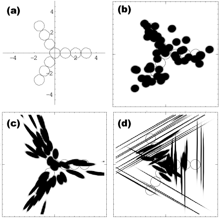
Figure 5: Same as Fig. 3 for an equiprobable star-shaped ensemble of 10 coherent states (STAR).

Finally, in the case of the STAR ensemble, the differences between the three visualizations are even more striking. As usual, the heterodyne scheme’s coherent states are scattered around the three lobes of the original ensemble (Fig. 5(b)). So are the phase-squeezed states of Wiseman’s scheme (Fig. 5(c)), but they are so elongated in the radial direction that they are almost incapable of distinguishing different states from the same lobe. Interestingly, the average information gain of Wiseman’s scheme is only slightly larger than $\log_{2}3\approx 1.585$, which may be interpreted to result from perfect discrimination of the phase of each coherent state, but very poor discrimination in the amplitude of coherent states from the same lobe.

The visualization of the LMMI measurement of the STAR ensemble predominantly consists of highly squeezed states that are perpendicular to the three lobes of the ensemble. The LMMI scheme therefore first quickly determines the phase of a given state, and then performs homodyne measurement of its amplitude. As a result, it performs noticeably better than both the heterodyne scheme and Wiseman’s scheme, covering a significant fraction of information gap between the performances of the heterodyne scheme and the best quantum measurement, as specified by the Holevo information of the ensemble.

V Discussion and conclusions

The purpose of this study was to present a new adaptive detection technique and explore some of its properties rather than conduct an exhaustive numerical analysis of its performance. Therefore, I presented the simulation results for only three ensembles that were specifically chosen to highlight the properties of the considered measurement schemes. In all of them, the LMMI scheme statistically outperforms both the heterodyne and Wiseman’s schemes. Nevertheless, this seems to be a general result. While I have performed similar simulations with other ensembles of coherent states, I have never found an ensemble where the LMMI scheme would perform worse than either the heterodyne or Wiseman’s scheme.

It is clear from the discussion above that adaptive measurements generally make a good use of prior measurement results in determining the optimal local oscillator phase. Wiseman’s scheme is designed to measure the phase and therefore performs particularly well with phase-modulated ensembles. The LMMI scheme is more versatile in that it can measure the phase as well as Wiseman’s scheme but can also perform other types of adaptive homodyne measurements when the ensemble features call for it.

As a price for its better performance, the LMMI scheme is much more demanding computationally, as probabilities have to be updated after each step and the new phase calculated according to the relatively complicated Eq. (10). This reflects a traditional tradeoff between information capacity and computational complexity that is typical of many communication problems. However, with the ever increasing speed and decreasing cost of computing power, the general trend has recently been towards more sophisticated schemes that can extract more information from imperfect channels.

The analysis presented in this paper can be relatively easily generalized to include the case of unequal a priori probabilities and noisy photodetectors, but the results are qualitatively similar to the ones discussed above. Note that adaptive schemes generally seem to be more robust with respect to instrumental imperfections than nonadaptive ones geremia . In the future, it would be interesting to extend the analysis to squeezed states and determine whether it is possible to beat the homodyne limit ${\cal I}_{2}(\left<n\right>)$ with adaptive measurements of ensembles of, for example, phase-squeezed states. It would also be instructive to prove or disproof the global optimality of the LMMI measurement scheme, but like any nonlinear global optimization problem, it is probably a difficult task.

In conclusion, I have studied extraction of classical information from an ensemble of coherent states using a new adaptive measurement scheme that maximizes the average information gain (mutual information) at each step of the adaptive measurement. Judging from the three considered examples, the proposed LMMI scheme is quite versatile and adapts the measurement process to the features of each ensemble. As a result, the LMMI scheme consistently outperforms heterodyne detection and Wiseman’s adaptive scheme. In the case of the 16QAM and STAR ensembles, the improvement in extracted information with respect to the heterodyne scheme was 4% and 18%, respectively. In the case of the 8PSK ensemble, the average information gains of Wiseman’s and LMMI adaptive schemes are almost equal and about 13% larger than the average information gain of the heterodyne detection. In the latter case, the two adaptive schemes even surpass the limit of heterodyne detection for the same average number of photons per pulse. Compared to Wiseman’s adaptive scheme, the LMMI scheme is more computationally intensive, but its superior performance and versatility may well justify its use for ensembles of weak coherent states.

References

- (1) J. G. Proakis, Digital communications (New York: McGraw-Hill, 2001).
- (2) L. Mandel, E. Wolf, Optical coherence and quantum optics (New York: Cambridge Univ. Press, 1995).
- (3) N. Gisin, G. Ribordy, W. Tittel, H. Zbinden, Rev. Mod. Phys. 74, 145 (2002).
- (4) V. Vilnrotter, C.-W. Lau, Quantum Detection Theory for the Free-Space Channel, The InterPlanetary Network Progress Report 42-146, Jet Propulsion Laboratory, Pasadena, CA (2001).
- (5) C. M. Caves, P. D. Drummond, Rev. Mod. Phys. 66, 481 (1994).
- (6) In principle, there is no difference between continuous adaptive homodyne and continuous adaptive heterodyne measurements since both allow an arbitrary dependence of local oscillator phase on the prior detection record. I call the measurements considered in this paper homodyne only because in the discrete realizations simulated below, the detection is homodyne during each step of the measurement.
- (7) D. T. Pope, H. M. Wiseman, N. K. Langford, Phys. Rev. A 70, 043812 (2005).
- (8) M. A. Armen, J. K. Au, J. K. Stockton, A. C. Doherty, H. Mabuchi, Phys. Rev. Lett. 89, 133602 (2002).
- (9) K. Kato, M. Osaki, IEEE Trans. Commun. 47, 248 (1999).
- (10) J. M. Geremia, Phys. Rev. A 70, 062303 (2004).
- (11) H. M. Wiseman, Phys. Rev. Lett. 75, 4587 (1995).
- (12) M. Osaki, O. Hirota, M. Ban, J. Mod. Opt. 45, 269 (1998); M. Osaki, T. Sasaki-Usuda, O. Hirota, Phys. Lett. A 245, 189 (1998).
- (13) John Preskill, Lecture notes on Physics 229: Quantum information and computation, located at Caltech website http://www.theory.caltech.edu/people/preskill/ph229/
- (14) P. W. Shor, IBM J. Res. Dev. 48 115 (2004).
- (15) M. Sasaki, S. M. Barnett, R. Jozsa, M. Osaki, O. Hirota, Phys. Rev. A 59, 3325 (1999).
- (16) P. Hausladen, W.K. Wootters, J. Mod. Opt 41, 2385 (1991).
- (17) H. M. Wiseman, R. B. Killip, Phys. Rev. A 56, 944 (1997).
- (18) Of course, should not be so small that the discrete nature of photocounts begins to play a role. This can be avoided if the local oscillator is sufficiently strong.
- (19) M. B. Plenio and P. L. Knight, Rev. Mod. Phys. 70, 101 (1998).
- (20) H. M. Wiseman, Quantum Semiclass. Opt. 8, 205 (1996).