Transverse localization and slow propagation of light

Abstract

The effect of finite control beam on the transverse spatial profile of the slow light propagation in an electromagnetically induced transparency medium is studied. We arrive at a general criterion in terms of eigenequation, and demonstrate the existence of a set of localized, stationary transverse modes for the negative detuning of the probe signal field. Each of these diffraction-free transverse modes has its own characteristic group velocity, smaller than the conventional theoretical result without considering the transverse spatial effect.

Ultraslow propagation of light fields has been an active research field recently. Controlling the light propagation in atomic and solid-state media is important in both the fundamental theory and practical applications of nonlinear optics rev . Slow light propagation experiments have been reported by using ultracold atoms Hau99 ; Inouye00 ; kane04 , hot atoms Kash99 ; Budker99 , rare-earth ion doped crystal turukhin02 , ruby bigelow03a , and alexandrite crystals bigelow03b . The use of electromagnetically induced transparency (EIT) to obtain slow light propagation is one of the most important techniques. In an EIT medium eit , when a control laser is applied to an appropriate transition, a weak probe signal pulse may have small absorption and steep dispersion. Due to this steep dispersion, the group velocity of the signal pulse can be reduced to several orders smaller than the light speed in vacuum Hau99 ; Inouye00 ; kane04 ; Kash99 ; Budker99 ; turukhin02 . Further, by changing the intensity of the control laser, it is possible to reversibly stop the signal pulse polarit . Stop light propagation has been observed in cold and hot alkali vapors liu01 ; phillips01 . Possible applications of slow light include the enhancement of nonlinearity Schmidt96 ; Harris98 ; Masalas04 , entanglement of atomic ensembles or photons Lukin00a ; Lukin00b , quantum memories qmemo , and optical information processing infbec .

Almost all theoretical treatments so far involve the assumption of an effective infinite transverse spatial variation of control field, and how a finite transverse profile affects the light propagation in an EIT medium is yet to be addressed. An exception is the work in Ref. Andre04, . The authors investigated the transverse localization of the stationary probe pulses with a pair of counter-propagating control fields, and showed it is possible to realize a three-dimensional confinement of the probe pulses Andre04 . The focus of Ref. Andre04, was how to localize light pulses in three dimensions. In this paper, we are interested in the transverse effects on slow light propagation. In particular, we arrive at a general criterion in terms of eigenequation for the transverse stationary modes of the signal field. These transverse modes exist only at negative detuning frequency region, and do not undergo diffraction, thus keeping their profiles during the propagation. The group velocity of each stationary mode will also be studied quantitatively.

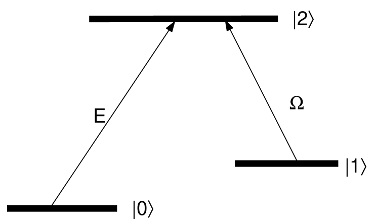
Figure 1: The three-level $\Lambda$-type EIT medium. $\Omega$ is the Rabi frequency of the classical control field, and $E$ is the electric field of the probe signal pulse.

We start with the three-level $\Lambda$-type atoms shown in Fig. 1. The medium of length $L$ consists of an ensemble of $N$ atoms. The ground state $|0\rangle$ and the metastable Stokes state $|1\rangle$ are coupled individually with the excited state $|2\rangle$ via a weak probe signal pulse and an intense control laser field, respectively. The latter is treated classically and assumes the form $\mathcal{E}_{c}(z,t,\vec{r})=\Omega(z,t,\vec{r})e^{i(k_{c}z-i\omega_{c}t)}$, where $\Omega(z,t,\vec{r})$ denotes the Rabi frequency and $k_{c}=\omega_{c}/c$, with the carrier frequency, $\omega_{c}=\omega_{12}$, being set to be on resonance with the Stokes transition. The weak signal field shall be treated as a quantum field polarit :

$$\hat{{\mathcal{E}}}(z,t,\vec{r})=\hat{E}(z,t,\vec{r})e^{i(k_{0}z-i\omega_{02}t)},$$ (1)

where $k_{0}\equiv\omega_{02}/c$. The probe carrier frequency $\omega_{s}$ is assumed to be close to the $|0\rangle\to|2\rangle$ transition frequency $\omega_{02}$. In Eq. (1), $\hat{E}(z,t,\vec{r})$ denotes the slowly varying signal field envelop operator. Following Ref. polarit, , but including now also the finite control beam effects, the signal pulse in the paraxial approximation and slowing varying amplitude approximation can be describe by the propagation equation,

$$\left(\frac{\partial}{\partial t}+c\frac{\partial}{\partial z}-i\frac{c\nabla_{\rm T}^{2}}{2k_{0}}\right)\hat{E}=igN\hat{\sigma}_{02}(z,t,\vec{r}).$$ (2)

Here, $\nabla_{\rm T}^{2}=\nabla^{2}-\frac{\partial^{2}}{\partial z^{2}}$ is the transverse Laplacian, $g=\mu_{02}\sqrt{\frac{\omega_{02}}{2\hbar\epsilon_{0}V}}$; with $\mu_{02}$ being the transition dipole moment and $V$ the quantization volume, denotes the atom-field coupling constant for $|0\rangle\to|2\rangle$, while $\hat{\sigma}_{02}$ is a slowly varying collective operator of the atoms. In general, $\hat{\sigma}_{ij}(z,t,\vec{r})=\frac{1}{N_{\vec{r}}}\sum_{l=1}^{N_{z,\vec{r}}}|i\rangle_{l}\langle j|e^{-i\omega_{ij}t}$, where the sum runs over the effective number of atoms in a small but macroscopic volume around position $\vec{r}$ Andre04 .

We shall be interested in the case in which the Rabi frequency of the signal field is much smaller than that of the control field $\Omega$ and the number of input probe photons is much less than that of atoms. In the adiabatic approximation, $\hat{\sigma}_{02}(z,t,\vec{r})=\frac{ig}{\Omega}\frac{\partial}{\partial t}\frac{\hat{E}(z,t,\vec{r})}{\Omega}$ polarit ; Andre04 , leading Eq. (2) to

$$\left(\frac{\partial}{\partial t}+c\frac{\partial}{\partial z}-i\frac{c\nabla_{\rm T}^{2}}{2k_{0}}\right)\hat{E}=-\frac{g^{2}N}{\Omega}\frac{\partial}{\partial t}\frac{\hat{E}(z,t,\vec{r})}{\Omega}$$ (3)

In most experiments, the control field is continuous and has a cylindrical symmetry transverse spatial profile $\Omega(r)$ that changes little in the propagation direction. To study the transverse effects of the probe signal field in this case, we consider the expectation value of $\hat{E}(z,t,\vec{r})$ in terms of

$$E(z,t,\vec{r})=\psi(r)e^{im\theta}e^{i(\Delta z-\delta t)},$$ (4)

with the quantum number $m=0,\pm 1,\cdots$ for the orbital angular momentum of the signal field OAM . The signal wavevector mismatch $\Delta\equiv k_{s}-k_{0}$ along the $z$-direction will be determined as the function of frequency detuning $\delta\equiv\omega_{s}-\omega_{02}$. Equation (3) can then be reduced to

$$\left[-\frac{d^{2}}{dr^{2}}-\frac{1}{r}\frac{d}{dr}-\frac{2k_{0}g^{2}N\delta}{c\Omega^{2}(r)}+\frac{m^{2}}{r^{2}}\right]\psi(r)=\beta\psi(r),$$ (5)

where the eigenvalue $\beta\equiv 2k_{0}(\delta/c-\Delta)$ defines the dispersion relation between $\Delta$ and $\delta$ for each transverse mode of the signal field. The physical boundary conditions for Eq. (5) are $\psi(\infty)=\psi^{\prime}(0)|_{m=0}=\psi(0)|_{m\neq 0}=0$.

It is noted that Eq. (3) may be considered as a propagation version of Eq.(2) in Ref. Andre04, (by setting $\Omega_{-}=0$ there). However, our work and Ref. Andre04, have different physical background. Ref. Andre04, was focused on how to realize light localization. The novel result of this paper is Eq. (5). It unambiguously shows the general properties of a complete set of transverse invariant eigenmodes for slow light propagation in the EIT medium.

For a negative detuning ($\delta<0$), the eigenequation (5) for each integer value of $m$ is quantized. The resulting transverse modes and eigenvalues are denoted as $\psi_{mn}(r)$ and $\beta_{mn}$, respectively; with $n=1,2,\cdots$ and $0<\beta_{m1}<\beta_{m2}<\cdots$ for each $m=0,\pm 1,\cdots,\pm(n-1)$. Physically, the negative frequency detuning leads to the decrease of the refractive index from the optical axis and the production of an effective waveguide for the signal field. The group velocity for each stationary transverse mode of the signal field can be evaluated via its eigenvalue as

$$V_{g}^{mn}=\left(\frac{\partial\Delta}{\partial\delta}\right)^{-1}=\left(1-\frac{c}{2k_{0}}\frac{\partial\beta_{mn}}{\partial\delta}\right)^{-1}c.$$ (6)

For a given control field with an arbitrary transverse profile and the relevant parameters for the optical medium, one can solve Eq. (5) to obtain all eigenvalues $\beta_{mn}$ and the corresponding transverse modes $\psi_{mn}(r)$. Any localized input probe signal pulse $E(0,t,\vec{r})$ can be expanded as the superposition of these transverse modes; each of these modes then propagates at its own distinct velocity, and thus, the signal pulse of superposition changes its spatial-temporal profile during the propagation. Clearly, if the input pulse is characterized by a single transverse mode it will not undergo diffraction and remains the initial shape during the propagation.

In the following we use numerical simulations to demonstrate the effects of control light beam size on various stationary transverse signal modes with negative detuning. The transverse spatial profile of the control field is chosen to be Gaussian,

$$\Omega(r)=\Omega_{0}e^{-r^{2}/(2a^{2})}.$$ (7)

The reported results will be exemplified with $\Omega_{0}=10^{8}\,{\rm s}^{-1}$ and $a=50\,\mu{\rm m}$. The parameters of the medium are set to be $g^{2}N=10^{22}{\rm s}^{-2}$ for the atom density of $10^{14}\,{\rm cm}^{-3}$, and the $|0\rangle\to|2\rangle$ transition wavelength is 780 nm. The eigenmodes are normalized as $\int_{0}^{\infty}r|\psi_{mn}(r)|^{2}dr={\rm const}$.

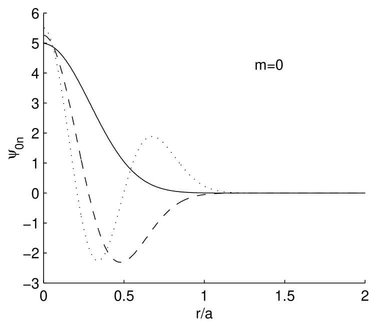
Figure 2: The lowest three transverse modes for $m=0$: $\psi_{01}(r)$ (solid), $\psi_{02}(r)$ (dash), and $\psi_{03}(r)$ (dot); with the probe signal detuning $\delta=-10^{6}\,{\rm s}^{-1}$. See text for the other parameters.

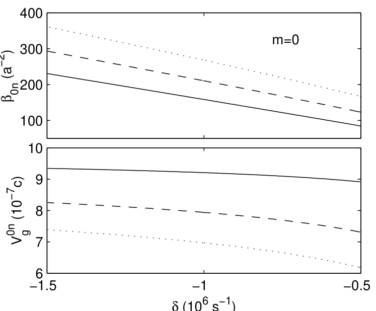
Figure 3: The eigenvalues (upper panel) and the corresponding group velocities (lower panel), for the transverse eigenmodes $\psi_{01}(r)$ (solid lines), $\psi_{02}(r)$ (dashed lines), and $\psi_{03}(r)$ (dotted lines), as the functions of detuning $\delta$. Other parameters are the same as in Fig. 2.

Figure 2 shows the radial profiles of the lowest three transverse modes, $\psi_{01}(r)$, $\psi_{02}(r)$, and $\psi_{03}(r)$; with $m=0$ and $\delta=-10^{6}\,{\rm s}^{-1}$. The lowest mode $\psi_{01}(r)$ decreases monotonically, while the higher mode $\psi_{0n}(r)$, with $n>1$, oscillates and has $(n-1)$ nodes. Here, we must point out that numerical calculations show that Gaussian function can well approximate the the ground mode ($\psi_{01}(r)$) Andre04 . Figure 3 depicts the eigenvalues $\beta$ (upper panel) and the corresponding group velocities $V_{g}$ (lower panel) of the lowest three transverse modes as functions of detuning $\delta<0$. For a given transverse mode, an increase in $|\delta|$ leads to an increase in $|\beta|$ (and also in wavevector mismatch), but a decrease in the group velocity $V_{g}$ as it is calculated according to Eq. (6). Note that if the effect of transverse spatial distribution is completely neglected, the group velocity for the present system would be $V_{g}=(1+g^{2}N/\Omega_{0}^{2})^{-1}c=10^{-6}c$, larger than the values we obtained here. It is also interesting to see that at a given negative detuning, a higher mode is of a smaller group velocity. Thus, by making use of a high-order transverse mode of the probe signal field with a small negative detuning frequency, it is possible to have a slow light propagation in an EIT medium.

We now study the transverse modes with nonzero orbital angular momentum, i.e., the eigenmodes of Eq. (5) with $m\neq 0$, which represent optical vortex. Note that $\psi_{-m,n}=\psi_{m,n}$ [c.f. Eq. (5)]. In Fig. 4, we plot the “ground” and the first “excited” modes for both $m=1$ and $m=2$: $\psi_{11}$ (thin-solid), $\psi_{12}$ (thin-dash), $\psi_{21}$ (thick-solid), and $\psi_{22}$ (thick-dash), for the same EIT system and field parameters of Fig. 2. The transverse mode $\psi_{mn}(r)$ is found to have $(n-1)$ nodes, besides that of $\psi_{m\neq 0,n}(0)=0$. For a given $n$, $\psi_{mn}(r)$ with a large $m$ extends to a large $r$. The negative detuning frequency dependences of these $m\neq 0$ modes are presented in Fig. 5. The qualitative properties are similar as Fig. 3. It is found that $V_{g}^{11}>V_{g}^{21}>V_{g}^{12}>V_{g}^{22}$. The group velocities for the transverse mode $\psi_{mn}$ satisfy in general

$$V_{g}^{m1}>V_{g}^{m2}>\cdots\ \ {\rm and}\ \ V_{g}^{1n}>V_{g}^{2n}>\cdots$$ (8)

at a given negative detuning, while each individual $V_{g}^{mn}(\delta)$ decreases as the negative detuning reduces.

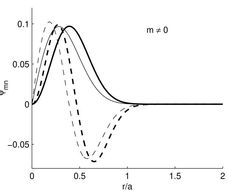
Figure 4: Some lowest transverse modes with finite orbital angular momentum $m$: $\psi_{11}(r)$ (thin-solid), $\psi_{12}(r)$ (thin-dash), $\psi_{21}(r)$ (thick-solid), and $\psi_{22}(r)$ (thick-dash). Other parameters are the same as in Fig. 2.

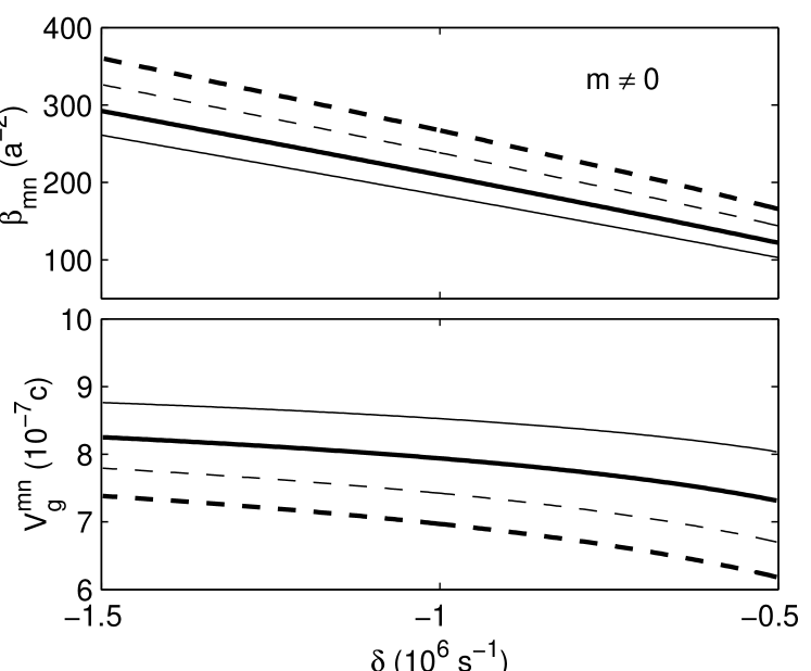
Figure 5: The eigenvalues (upper panel) and the group velocities (lower paner) for the eigenmodes of Fig. 4 as the functions of detuning frequency $\delta$.

All these calculated transverse mode velocities are smaller than the value of $10^{-6}c$, the group velocity with no consideration of the finite transverse distribution. Our calculations also conclude that the more focused (smaller $a$) the control field is, the smaller group velocity will be. On the other hand, as the size of the control field increases, the group velocity of each transverse eigenmode approaches to the asymptotic, transverse-effect-free value of $V_{g}=(1+g^{2}N/\Omega_{0}^{2})^{-1}c$, which is $10^{-6}c$ in the present EIT system of study. It also suggests that in order to observe the transverse effects experimentally, should not only the propagation length be long enough, but also the control field be well focused.

It is noticed that the transverse profile of the control field, $\Omega(r)$ may vary in a realistic propagation in the $z$-direction, but it is assumed to be stationary in our theoretical treatment. The justification here is the fact that the adiabatic approximation is applicable if $\Omega(r)$ is a slowly varying function of the propagating distance. As a result, the probe signal field prepared initially in an eigenmode $\psi_{m,n}(r)$ can stay in this mode at any distance $z$, as long as the adiabatic approximation is applicable. For a Gaussian control beam, the adiabatic approximation requires the propagating distance smaller than the Rayleigh length of the control beam. In our example, the Gaussian beam with a spread of $a=50\,\mu{\rm m}$ leads to a Rayleigh length of $10\,{\rm cm}$. Both the beam focusing size and propagation length parameters demonstrated here are well accessible in current experiments. Moreover, the stationary behavior of an eigenmode propagation of the signal field can sustain over a much longer distance, if a non-diffracting Bessel rather than a Gaussian control beam is used nondiff .

In conclusion, we have studied the transverse effects of the slow light propagation in EIT mediums. In terms of eigenequation, a criterion of localized transverse modes is given. Using this criterion, a complete set of transverse modes can be numerically calculated. Different transverse modes propagate with different group velocities; all are smaller than the limiting value calculated from the previous theory without the consideration of the transverse spatial effect. Increasing the size of the control field will decrease this velocity difference. Higher order, or larger orbital angular momentum mode will have smaller velocity. Our results will also play important roles in the coherent light propagation control in general. For example, in Ref. Andre04, , a transverse light guiding technique was used to obtain three-dimensional confinement of light pulses. A Gaussian approximation to the lowest transverse mode with zero orbital angular momentum ($\psi_{01}$) was given. With the method present in this work, we should be able to identify the relevant transverse eigenmodes there. By carefully manipulating the transverse profile of the signal pulse, generalized and efficient realizations of the controlled location and storage of photonic pulses will become possible.

Support from the National Natural Science Foundation of China (10404031), Shanghai Rising-Star Program, the K. C. Wong Education Foundation (Hong Kong), and the Research Grants Council of the Hong Kong Government (604804) is acknowledged.

References

- (1) A.B. Matsko et al., Adv. Atom. Mol. Opt. Phys. 46, 191 (2001); R.W. Boyd and D.J. Cauthier, Prog. opt. 43, 497 (2002); Y. Rostovtsev et al., Optics and Photonics News 13, No. 6, 44 (2002); R. Walsworth, S. Yelin, and M. Lukin, ibid. 13, No. 1, 50 (2002); M.D. Lukin, Rev. Mod. Phys. 75, 457 (2003).
- (2) L.V. Hau et al., Nature (London) 397, 594 (1999).
- (3) S. Inouye et al., Phys. Rev. Lett. 85, 4225 (2000).
- (4) H. Kane, G. Hernandez, and Y. Zhu, Phys. Rev. A 70, 011801 (2004).
- (5) M.M.Kash et al., Phys. Rev. Lett. 82, 5229 (1999).
- (6) D. Budker et al., Phys. Rev. Lett. 83, 1767 (1999).
- (7) A.V. Turukhin et al., Phys. Rev. Lett. 88, 023602 (2002).
- (8) M.S. Bigelow et al., Phys. Rev. Lett. 90, 113903 (2003);
- (9) M.S. Bigelow et al., Science 301, 200 (2003).
- (10) S.E. Harris, Phys. Today 50, No. 7, 36 (1997); M.D. Lukin, and A. Imamoglu, Nautre (London) 413, 273 (2001).
- (11) M. Fleischhauer and M.D. Lukin, Phys. Rev. Lett. 84, 5094 (2000);
- (12) C. Liu et al., Nature (London) 409, 490 (2001).
- (13) D. Phillips et al., Phys. Rev. Lett. 86, 783 (2001).
- (14) H. Schmidt and A.Imamoglu, Opt Lett. 21, 1936 (1996).
- (15) S.E. Harris and Y. Yamamoto, Phys. Rev. Lett. 81, 3611 (1998).
- (16) M. Maslas and M. Fleischhauer, Phys. Rev.A 69, 061801(R) (2004).
- (17) M.D. Lukin and A. Imamoglu, Phys. Rev. Lett. 84, 1419 (2000).
- (18) M.D. Lukin, S.F. Yelin, and M. Fleischhauer, Phys. Rev. Lett. 84, 4232 (2000).
- (19) M. Fleischhauer and M.D. Lukin, Phys. Rev. A 65, 022314 (2002); A.S. Zibrov et al., Phys. Rev. Lett. 88, 103601 (2002); A. Nazarkin, R. Netz, and R. Sauerbrey, Phys. Rev. Lett. 92, 043002 (2004).
- (20) Z. Dutton and L. V. Hau, Phys. Rev. A 70, 053831 (2004).
- (21) A. Andre et al., Phys. Rev. Lett. 94, 063902 (2005).
- (22) L. Allen, M.J. Padgett, M. Babiker, Prog. Opt. 39, 291 (1999).
- (23) J. Durnin, J. Opt. Soc. Am. A 4, 651 (1987).