Rydberg wavepackets in terms of hidden-variables: de Broglie-Bohm trajectories

Abstract

The dynamics of highly excited radial Rydberg wavepackets is analyzed in terms of de Broglie-Bohm (BB) trajectories. Although the wavepacket evolves along classical motion, the computed BB trajectories are markedly different from the classical dynamics: in particular none of the trajectories initially near the atomic core reach the outer turning point where the wavepacket localizes periodically. The reasons for this behavior, that we suggest to be generic for trajectory-based hidden variable theories, are discussed.

I Introduction

A Rydberg atom is an effective one-electron atom. Following laser excitation, a single electron (called the Rydberg electron) is excited and periodically returns to the region near the core (made up of the nucleus and the other tightly bound electrons). When the laser pulse is short-lived, a wavepacket is formed. Since they were first observed some 15 years ago rad1 ; rad2 , the production and detection of Rydberg wavepackets have become increasingly accurate, with developments pointing toward possible applications in quantum information bucksbaum00 or fundamental investigations such as the production of Schrödinger cat states noel stroud96 . To analyze Rydberg wavepacket propagation, the main theoretical frameworks from the early analysis averbukh-perelman down to the more sophisticated models zoller ; robinett have called for classical or semiclassical techniques and concepts, usually encapsulated within the path integral formulation of quantum mechanics: an initially localized and highly excited wavepacket is said to evolve along classical trajectories, the observed interferences being due to pieces of the wavepacket that travel along different classical trajectories.

An alternative interpretation of quantum phenomena hinges on the existence of particles each following a well-defined space-time trajectory. The de Broglie Bohm (BB) theory is by far the best-known and most developed of the trajectory-based hidden variable theories holland93 . BB trajectories have been determined for a wide range of quantum systems, including atom-surface diffraction sbm01 , quantum billiards alcantara00 , kicked rotators pla298 or even photons pla290 . Surprisingly, little has been done on Rydberg atoms gocinski99 ; pla04 and even there only elliptic states (angular wavepackets) were treated: BB trajectories for angular wavepackets were seen to closely approximate classical motion. However radial wavepackets are the most accessible experimentally, since they only require an optical excitation from the ground state of the atom. Indeed, most fundamental properties of wavepackets have essentially been investigated by forming radial, rather than angular wavepackets.

The object of this work is to analyze the dynamics of Bohmian particles in a radial wavepacket. To this end, we will sketch in Sec. 2 a realistic model of laser excitation resulting in the creation of a radial wavepacket in the hydrogen atom, also valid for other Rydberg atoms with a nonpenetrating outer electron (i.e. small quantum defects). We will give a brief overview of Bohmian dynamics (Sec. 3) and then compute the BB trajectories for the Rydberg electron (Sec. 4): we will see that the BB trajectories get quickly uncorrelated with the center of the wavepacket. In particular, none of the BB trajectories initially in the core region reach the outer tuning point, where the wavepacket localizes after half the classical period. The reasons for this behavior, some of which will be argued to be relevant to the model employed and others intrinsic to trajectory based hidden variable theories, will be discussed in Sec. 5. Our closing comments will be given in Sec. 6.

II Generation and propagation of Rydberg Wavepackets

We describe in this Section the excitation process leading to the creation of a wavepacket. We will insist on the main physical ideas (a detailed theoretical account may be found in zoller ). We assume the atom is initially in its ground state, that we take to be represented by the hydrogenic ground state wavefunction $1s$, radially given by a decreasing exponential with mean value $\bar{r}=1.5$ au and with negligible probability density for $r\gtrsim 5$ au (atomic units will be used throughout). The exciting laser pulse is described in the weak-interaction limit by the electric field $\mathbf{E}=\mathcal{E}(t)e^{-i\omega t}\mathbf{e}$, where $\omega$ is the laser frequency, $\mathbf{e}$ the polarization vector and $\mathcal{E}(t)$ the excitation enveloppe. For definiteness, we shall set $\mathbf{e}$ to be linearly polarized, $\omega$ to correspond to a transition to the Rydberg state $n=40$ and choose for the excitation profile a Gaussian enveloppe. Provided the duration $\tau_{P}$ of the Gaussian pulse is sufficiently short (much shorter than the recurrence time of the wavepacket), the wavefunction of our system can be written as zoller

$$\left|\psi(t)\right\rangle=\chi(t)\left|1s\right\rangle+\int_{-\infty}^{t}\left|\phi(t^{\prime})\right\rangle dt^{\prime},$$ (1)

where the time line has been set as follows. At $t=-\infty$ the atom is in the ground state; at $t=0$ the maximum of the pulse has reached the atom. $\chi(t)$ represents the depletion of the initial state that gets excited by the laser; it stands as a cut-off function, with $\chi(t\ll-\tau_{P}/2)=1$. Finally the second term on the right handside of Eq. (1) is the excited wavepacket. This term is of course zero for $t\ll-\tau_{P}/2$. On the other hand, for $t\gg\tau_{P}/2$, i.e. after the pulse excitation, it takes the form

$$\int_{-\infty}^{t\gg\tau_{P}/2}\left|\phi(t^{\prime})\right\rangle dt^{\prime}=\sum_{n}c_{n}e^{-iE_{n}t}\left|R_{n}\right\rangle\left|l=1,m=0\right\rangle,$$ (2)

where $\left|R_{n}\right\rangle$ is the hydrogenic radial wavefunction (regular Coulomb function) corresponding to principal quantum number $n$ and $l=1.$The coefficients $c_{n}$, which are related to the Fourier transform of the excitation enveloppe, take here the Gaussian form

$$c_{n}=d_{n}\exp\frac{(n-n_{0})^{2}}{2\Delta n^{2}}.$$ (3)

The center of the Gaussian distribution $n_{0}$ depends on the laser frequency $\omega$ (in this work we set $n_{0}=40)$ and the width $\Delta n$ on the pulse duration $\tau_{P}$. $d_{n}$ is the normalizing factor, which strictly speaking also depends on the dipole excitation strength to the excited states $\left|R_{n}\right\rangle\left|l=1,m=0\right\rangle.$

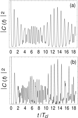
Figure 1: The autocorrelation function $|C(t)|^{2}$ (arbitrary units) for a wavepacket with mean energy $E_{0}$ is given as a function of time in units of the classical period of the electron for $n_{0}=40$, $T_{cl}\thickapprox 9.7$ ps. (a) corresponds to $\Delta n=.75$ and (b) to $\Delta n=1.5$, yielding a larger energy excitation window.

In short, the laser pulse creates a radial wavepacket whose expansion on the eigenstates is given by a Gaussian distribution. The wavepacket propagates outward, reaches the outer turning point and comes back toward the core region. The experimental generation and detection of such wavepackets is very common jones98 . The autocorrelation function is of particular interest. It is given by the overlap of the propagating wavepacket with the initially excited one,

$$C(t)=\left\langle\psi(t=0)\right|\left.\psi(t)\right\rangle=\sum_{n}\left|c_{n}\right|^{2}e^{-iE_{n}t}$$ (4)

and is straightforward to compute. Experimentally this quantity is directly detected by employing a second excitation laser jones98 .

Fig. 1 shows two examples of autocorrelation functions computed with the characteristics detailed above. The only difference is the pulse duration $\tau_{P}$ which is shorter in Fig. 1(b), leading to a wider excitation window $\Delta n$. This is why the wavepacket spreads faster. Still in both Figs. 1 (a) and (b), the characteristic time scales are visible: at short times the wavepacket is rather well-localized and the first peaks of $C(t)$ (in particular in Fig. 1(a)) are produced by the return of the wavepacket to the core at the classical period

$$T_{cl}(E_{0})=\pi 2^{-1/2}(-E_{0})^{3/2},$$ (5)

where $E_{0}=-1/2n_{0}^{2}$ is the energy of the center of the wavepacket. The classical periodicity arises from Eq. (4) by employing semiclassical arguments: in a WKB approach, expanding $E_{n}$ and using the WKB quantization condition gives the dependence $t/T_{cl}$ in the exponential averbukh-perelman ; robinett . Alternatively, imposing the stationary phase approximation in the Feynman path integral expression for propagator leads when $t$ is a multiple of $T_{cl}$ to isolated peaks or to a complex interference pattern, depending on whether different bits of the wavepacket carried by classical trajectories having different energies interfere appreciably. Another feature of the autocorrelation function concerns the revival phenomenon, particularly visible at $t/T_{cl}>13$ in Fig. 1(a), due to the fact that the different classical paths approximately recover the original phase relationships, yielding a wavefunction nearly identical to the original one. The position of the wavepacket at different times can also be computed (in principle it can also be detected experimentally burgdofer etal01 ). This has been done in Fig. 2, where the wavefunction is plotted at different times shortly after excitation. It can be seen that once a localized wavepacket gets formed it moves in accordance with classical dynamics. At $t=T_{cl}/2$, more than 99% of the wavefunction lies beyond $r=1600$ au.

Figure 2: Evolution of the radial wavepacket corresponding to case (b) of Fig. 1. Snapshots of the wavefunction are taken at different times. Each arrow shows the position at the corresponding time of an electron along a classical trajectory with initial position $r_{cl}=2$ au. The turning point for the center of the wavepacket lies at $r_{\mathrm{tp}}\thickapprox 3200$ au.

III Dynamics with a single hidden trajectory: De Broglie-Bohm mechanics

In his original paper Bohm bohm52 proposed an interpretation by which an individual quantum system has a ”precise behavior” in terms of hidden variables. The standard quantum formalism, that reaches an excellent agreement with the statistical distribution of measurements would thus be explained by averaging over a distribution of well defined but hidden trajectories. In the last decade, BB mechanics has become increasingly popular, and excellent accounts of the interpretation are available holland93 ; bohm hiley . The main dynamical equations arise from the polar decomposition of the wavefunction in configuration space. Put

$$\psi(\mathbf{r},t)=\rho(\mathbf{r},t)\exp(i\sigma(\mathbf{r},t))$$ (6)

where $\rho$ and $\sigma$ are real functions. The Schrödinger equation becomes equivalent to the coupled equations

$$\frac{\partial\sigma}{\partial t}+\frac{(\triangledown\sigma)^{2}}{2}+V-\frac{\triangledown^{2}\rho}{2\rho} =0$$ (7)

$$\frac{\partial\rho^{2}}{\partial t}+\triangledown(\rho^{2}\triangledown\sigma) =0.$$ (8)

$\rho^{2}$ gives the statistical distribution of the particle (here the Rydberg electron) whereas the trajectory is obtained by integrating the equation of motion

$$\frac{d\mathbf{r}}{dt}=\mathbf{\triangledown}\sigma(\mathbf{r},t)$$ (9)

where the initial position of the electron $\mathbf{r}(t=-\infty)$ lies within the initial distribution $\rho(t=-\infty).$

As should be expected from any theory that accounts for quantum dynamics by employing a single trajectory, there is a close relationship between the motion of the putative particle and the net probability current. Eq. (8) expresses the conservation of the probability flow. For an energy eigenstate of a Rydberg atom, there is no net probability flow in the radial coordinate and according to Eqs. (6)-(8) the electron has no radial motion. This is dynamically explained by the last term on the right handside of Eq. (7),

$$Q(\mathbf{r},t)=-\frac{\triangledown^{2}\rho}{2\rho}$$ (10)

known as the quantum potential, that cancels the effects of the classical potential $V$.

It is thus interesting to compute BB trajectories for time dependent wavepackets and to give an interpretation of an observable quantity such as the autocorrelation function in terms of the statistical distribution of hidden but well-defined electron trajectories. This is readily done by casting the Rydberg wavepackets obtained in Sec. 2 in the form of Eq. (6). Since we have set $m=0$, $\sigma(\mathbf{r},t)$ has no contribution from the angular coordinates and there is no angular motion: once an initial position has been set for the particle, the electron incurs only a radial motion. Eq. (9) is thus simply one dimensional. However it is still demanding to solve it because the equation of motion is extremely sensitive to the position of the nodes of the wavefunction. Not only do highly excited eigenstates, from which the wavepacket is built, have a great number of nodes, but the ’quasi-nodes’ of the wavepacket can move very quickly in particular during the application of the laser pulse.

IV Results

We have numerically integrated Eq. (9) for the two Rydberg wavepackets (a) and (b) of Sec. 2. The resulting de Broglie-Bohm trajectories are shown in Fig. 3. We have chosen as the initial condition $r_{BB}(t=-\infty)=2$ au. Recall that the initial state $\left|1s\right\rangle$ is compactly localized around the core ($0<r\lesssim 10,$ $\bar{r}=1.5$ au) and that BB trajectories cannot cross: if initially $r_{1}(-\infty)>r_{2}(-\infty)$ then $r_{1}(t)>r_{2}(t)$ for all $t$. During the application of the laser pulse $r_{BB}(t)$ varies erratically back and forth around the initial position with a small amplitude. The particle then starts to move outward appreciably (for $t\gtrsim T_{cl}/10$). At $t\approx T_{cl}/2$, $r_{BB}$ reaches a maximum value $r_{BB}^{\max}$ (much larger for the case (b) wavepacket) and turns back toward the core. Indeed at that time the wavepacket has reached its maximum distance from the core and is localized around the classical outer turning point $r_{\mathrm{tp}}=3200$ au (see Fig. 2). Note however that $r_{BB}^{\max}\ll r_{\mathrm{tp}}$: the BB trajectory never reaches the outer turning point. This remains true whatever the initial position $r_{BB}(t=-\infty)$ of the electron (but see Discussion below). At $t=T_{cl}$ part of the wavepacket has returned to the core, producing a peak in the autocorrelation function (Fig. 1); the BB trajectory has also returned to the core region, $r_{BB}(T_{cl})$ being slightly larger than $r_{BB}(-\infty)$.

For longer times, the trajectories obtained for the wavepackets (a) and (b) are very different reflecting the difference in the quantum potential arising from the difference in the interference pattern (remember the only difference between the wavepackets (a) and (b) is the excitation window $\Delta n$). This is illustrated in the insets in Figs. 3(a) and 3(b) for the interval $2<t/T_{cl}<3$: in case (b) $r_{BB}(t)$ oscillates back and forth several times whereas in case (a) the trajectory makes a single round trip from the core, reflecting the classical periodicity. Note also that the revivals observed in the autocorrelation function (Fig. 1) are not neatly visible in the behavior of the BB trajectories. The reason is that revivals occur when the wavepacket approximately regain its initial shape, but then the quantum potential can be quite different.

Figure 3: Trajectories $r_{BB}(t)$ computed according to de Broglie-Bohm dynamics. (a) shows the trajectory with initial position $r_{BB}=2$ au as a function of time for the wavepacket (a) (see Fig. 1). The inset zooms on the interval $2<t/T_{cl}<3$ and in addition shows in grey (or color) BB trajectories evolved from different initial positions: from top to bottom the initial positions corresponding to the trajectories in the inset are 10 (yellow), 6 (blue), 2 (black) and 1 (red) au. (b): same as (a) but for the case (b) wavepacket.

Fig. 4 shows the situation for short times, i.e. when the wavepacket is still fairly well localized, for the case (b) wavepacket. The classical and Bohmian trajectories are plotted along with the average position of the wavepacket (expectation value of the position operator). The situation portrayed in Fig. 4 is an application of Ehrenfest’s theorem: before the break time the wavepacket evolves along a classical trajectory, whereas as can be easily shown (see Sec. 3.8 of holland93 ) BB trajectories generically never move with the wavepacket.

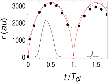
Figure 4: Short-time evolution of classical and Bohmian trajectories and average position of the wavepacket for the case (b) wavepacket. The black solid line is the BB trajectory with initial value $r_{BB}=2$ au already shown in Fig. 3(b), and the gray (red) line is the classical trajectory with the same initial position. The black dots represent the average position of the wavepacket. The dashed line is the BB trajectory that reaches the outer turning point region along with the wavepacket. Its ’initial’ (at $t=0$) position is $r\simeq 1000$ au. 

V Discussion

We have seen that the BB trajectories computed above have a striking property: no trajectory lying initially in the core region ever reaches the region near the outer turning point where the wavepacket periodically gets localized. We now discuss to what extent this is a feature specific to the present model or can be said to be an intrinsic aspect of the de Broglie-Bohm dynamics, or more generally of trajectory-based hidden variable theories.

The model summarized in Sec. 2 above is the most widely employed model describing Rydberg excitation by a tailored laser pulse. Crudely speaking, the excited wavepacket is progressively turned on: it is given by Eq. (2) multiplied by some function $\zeta(t)$ whose exact form depends on $\mathcal{E}(t),$ but that obeys $\zeta(t)=0$ for $t<-\tau_{P}/2$ and goes to $\zeta(t)=1$ for $t>-\tau_{P}/2$. Now the wavefunction given by Eq. (2) at $t=0$ is far from being perfectly localized near the origin and has a small but non-negligible probability density even at large $r$. This means that at say $r=1000$ au, although initially ($t<-\tau_{P}/2$) there is zero probability density, a small probability density appears as $\zeta(t)$ increases, which in a sense ’pops out’ of nowhere. This feature arises from the model employed to describe the wavepacket. In BB terms, this gives rise to trajectories such as the dashed line of Fig. 4, which obeys $r_{BB}(t=0)=1000\;$au. For such a trajectory it is numerically impossible to integrate the equation of motion backwards in time for $t\ll 0$ since the probability vanishes as $t\rightarrow-\infty$ (but clearly there cannot be any significant motion from the position at $t=0$ given that the nodes on each side of that initial position do not move as $t\rightarrow-\tau_{P}/2$ although the probability amplitude does decrease to $0$). Note that within the de Broglie-Bohm interpretation these type of trajectories need to be taken into account for consistency, because it is only by including them that the quantum mechanical expectation values can be matched to the statistical average over the ensemble of trajectories, as required by the theory.

However, the fact the hidden-variable BB trajectory does not follow the apparent dynamics of the wavepacket, which when localized moves in accordance with the classical trajectory, is unrelated to any specific model of wavepacket propagation. Let us take an eigenstate of the Hamiltonian: it is a standing-wave, which except for a global phase-factor (none in the present example because $m=0$) is a real function. According to the de Broglie-Bohm theory, there is no motion in that situation, the particle being at rest by Eq. (9). This is generically true of any theory positing a single trajectory dynamics depending on the net probability flow, which vanishes for stationary states. On the other hand, according to the path integral formalism, the standing wave arises from the interference of two waves travelling in the opposite directions; from the semiclassical approximation to the propagator, the waves follow the sole classical periodic orbit of the system, but interfere. It is clear that positing a single trajectory in space-time to account for quantum phenomena proscribes the possibility for such a trajectory to follow classical motion if interference effects are important.

The last remark also holds for an arbitrary wavepacket. Although the average position of the wavepacket follows the classical trajectory very quickly (Fig. 4), the wavepacket only starts to get localized for $t\gtrsim T_{cl}/4$, as illustrated in Fig. 2. At short times, when the wavepacket is formed, interference effects are very important. Locally the net probability flow may be insignificant, although the probability density is large. According to BB theory, the electron can then hardly move, because it is ’trapped’ by the nodes arising from the interference terms. By the time the BB particle moves away, the bulk of the wavepacket is already far ahead. Indeed, the net probability flow is delayed relative to the localized part of the wavepacket. At subsequent times the localized part of the wavepacket accounts for only a fraction of the total probability density and its motion is thus uncorrelated with the maximal probability flow. For example in the autocorrelation function shown in Fig. 1(a), the classical periodicity is clearly visible at short times, though only a small fraction of the total wavefunction returns to the core. If one postulates that the fundamental dynamics relies on the existence of a single hidden trajectory, whose dynamical law is directly related to the net probability flow, it is not possible to account for the classical periodicity (that can be experimentally observed) by invoking a correspondence with classical dynamics. Another illustration is afforded by the insets in Fig. 3. The BB trajectories in 3(a) and 3(b) are markedly different due to the local space-time structure of the probability flow. In contrast, the usually employed semiclassical framework ascribes the same underlying classical dynamics to both wavepackets, the only difference being the dispersion rate.

VI Conclusion

We have investigated highly excited radial Rydberg wavepackets in terms of hidden-variables trajectories obtained within the de Broglie-Bohm framework. The Bohmian picture of Rydberg atoms is internally consistent and compatible with the experimentally observed autocorrelation function. However contrarily to angular Rydberg wavepackets gocinski99 ; pla04 , the BB trajectories have little in common with classical motion. We have suggested that this is a generic feature of hidden variable theories accounting for quantum phenomena by the existence of a localized particle following a single trajectory. On the other hand we have also seen that the most commonly employed framework to interpret excited wavepacket phenomena hinges on semiclassical arguments, by which the dynamics is classical but the different paths interfere as the wavepacket spreads.

References

- (1) A. ten Wolde, L. D. Noordam, A. Lagendijk, and H. B. van Linden van den Heuvell, Phys. Rev. Lett. 61, 2099 (1988).
- (2) J. A. Yeazell, M. Mallalieu, J. Parker, and C. R. Stroud, Jr., Phys. Rev. A 40, 5040 (1989).
- (3) J. Ahn, T.C. Weinacht, and P.H. Bucksbaum, Science 287, 463 (2000).
- (4) M. W. Noel and C. R. Stroud, Jr., Phys. Rev. Lett. 77, 1913 (1996).
- (5) I. Sh. Averbukh and N. F. Perelman, Phys. Lett. A 139, 449 (1989). M. Nauenberg, J. Phys. B 23, L385 (1990).
- (6) G. Alber and P. Zoller, Phys. Rep. 199, 231 (1991).
- (7) R. W. Robinett, Phys. Rep. 392, 1 (2004).
- (8) P.R. Holland, The Quantum Theory of Motion, Cambridge Univ. Press, Cambridge (1993).
- (9) A. S. Sanz, F. Borondo and S. Miret-Artes, Europhys. Lett., 55, 303 (2001).
- (10) O. F. de Alcantara Bonfim, J. Florencio and F. C. Sa Barreto, Phys. Lett. A 277, 129 (2000).
- (11) G. E. Bowman, Phys. Lett. A 298, 7 (2002).
- (12) P. Ghose, A. S. Majumdar, S. Guha and J. Sau, Phys. Lett. A 290, 205 (2001).
- (13) H. Carlsen and O. Goscinski, Phys. Rev. A 59, 1063 (1999).
- (14) A. Datta, P. Ghose and M.K. Samal, Phys. Lett. A 322, 277 (2004).
- (15) R. R. Jones and L. D. Noordam, Adv. At. Mol. Opt. Phys. 38, 1 (1998).
- (16) B.E. Tannian, C. L. Stokely, F. B. Dunning, C. O. Reinhold and J. Burgdorfer, Phys. Rev. A 64 021404 (2001).
- (17) D. Bohm, Phys. Rev. 85, 166 (1952).
- (18) D. Bohm and B. J. Hiley, The Undivided Universe, Routledge, London, 1993.