Measures and dynamics of entangled states

Abstract

We develop an original approach for the quantitative characterisation of the entanglement properties of, possibly mixed, bi- and multipartite quantum states of arbitrary finite dimension. Particular emphasis is given to the derivation of reliable estimates which allow for an efficient evaluation of a specific entanglement measure, concurrence, for further implementation in the monitoring of the time evolution of multipartite entanglement under incoherent environment coupling. The flexibility of the technical machinery established here is illustrated by its implementation for different, realistic experimental scenarios.

1 Introduction

Entanglement is one of the central issues of debate in quantum theory since the beginning of the last century and certainly a key idea when it comes to distinguish classical and quantum concepts. Moreover, besides this fundamental aspect, the interest in entangled states has been recently renewed because their properties lie at the heart of many potential applications. Be it in quantum computation [1, 2], teleportation [3] or quantum cryptography [4], entanglement is viewed as an important resource and, as such, must be quantified. In addition, great experimental progresses in the production, manipulation and detection of entangled states [5, 6, 7, 8, 9, 10, 11, 12, 13, 14, 15, 16, 17] require such a quantification to be versatile enough to deal with the states encountered in actual experiments, which are in general mixed and typically involve several particles.

The first attempt to discern the non-local correlations of measurement results induced by entanglement was formulated with Bell’s inequalities [18, 19], which underwent a first experimental check [20] in the sixties. Bell’s inequalities are capable of discriminating correlations due to entanglement against those described by local hidden variable models [21]. Later, also entanglement criteria that use special three-partite states, without involving inequalities, were found [22] and tested experimentally [7]. Albeit able to reveal the entangled nature of some quantum states, the above criteria cannot (and do not intend) to quantify the amount of entanglement carried by a given state.

Only recently has the problem of finding a quantity that measures quantum correlations been studied more intensively [23, 24, 25]. Virtually the entire state-of-the-art theory of entangled quantum states is based on so-called entanglement measures, scalar quantities that quantify quantum correlations, and distinguish them from classical ones. For bipartite pure states such measures exist and are straightforwardly computable. However, if one aspires to describe realistic states observed in experiments, it is imperative to allow for a proper quantification also of mixed states entanglement, since there is no system that could be decoupled perfectly from environmental influences, and mixing is thus unavoidable.

Although several measures for mixed states have been proposed, no simple criterion of discriminating classical from quantum correlations is known so far. All proposed measures that unambiguously fulfill this task involve some - generally high dimensional - optimisation procedure, and hardly allow for an explicit evaluation in concrete cases. Only for states of smallest possible dimensions, i.e., for bipartite two-level systems, do a few measures exist that can be evaluated algebraically [27, 28, 29], though no such measures are known for arbitrary states of higher dimensional systems.

Hence, there is some mismatch between the more formal part of entanglement theory, which seeks for the general characterisation of arbitrary quantum states, and experimental progresses of the last years, which are leading to the production of (possibly specific classes of) ever more complex entangled states of multipartite quantum systems. For a theoretical analysis of the latter, we need algebraic as well as numerical tools to describe static as well as dynamical properties of multipartite quantum states in a quantitative manner – what is a nontrivial target, due to the rapidly increasing complexity of the problem at hand, as particle number and effective Hilbert space dimensions are increased. Studying the dynamics of entanglement requires efficiently evaluable quantifiers thereof as an undispensible ingredient, ideally for arbitrary system sizes.

In the present review, we attempt to improve on this mismatch, by responding precisely to this latter requirement: Starting from the formal algebraic description of a suitable entanglement measure – concurrence –, we derive a hierarchy of bounds [30] and approximations [31] thereof, which imply progressively reduced computational efforts for its actual evaluation for bi- or multipartite, mixed quantum states in arbitrary finite dimensions. After numerical tests of the tightness of these various estimates, we implement this novel toolbox, to monitor entanglement dynamics under experimentally realistic conditions [32].

We start out with a brief recollection of the most important concepts of entanglement theory.

1.1 Entangled states

1.1.1 Bipartite entanglement

A bipartite system is a quantum system that is composed of two physically distinct subsystems. It is associated with a Hilbert space ${\cal H}$ that is given by the tensor product ${\cal H}_{1}\otimes{\cal H}_{2}$ of the predefined factor spaces, each of which describes one subsystem.

For pure states one distinguishes two different kinds of states. A state $|\Psi\rangle$ is called a product state or separable, if it can be written as a tensor product of subsystem states, i.e. if there are states $|\varphi\rangle$ and $|\phi\rangle$ of the subsystems such that

$$|\Psi\rangle=|\varphi\rangle\otimes|\phi\rangle\ .$$ (1)

Such a state describes a situation analogous to a classical one insofar as the system state contains exactly the information that is contained in the subsystem states. A state reduction [33] caused by a measurement performed on one subsystem has no influence on the state of the other subsystem. This means that measurement results on the different subsystems are uncorrelated (or independent). In contrast to this, they are correlated for entangled states, i.e. states that cannot be written as a product of subsystem states as in Eq. (1). Here, a local measurement causes a state reduction of the entire, i.e. bipartite, system state, and therefore changes the probabilities for potential future measurements on either subsystem.

For mixed states the situation is more complicated. Product and separable states are not synonymous anymore. Whereas the former can be expressed as a tensor product of subsystem states, i.e. there are states $\varrho_{1}$ and $\varrho_{2}$ describing the single subsystems, such that

$$\varrho=\varrho_{1}\otimes\varrho_{2}\ ,$$ (2)

a convex sum of such product states is needed to represent a general separable state

$$\varrho=\sum_{i}\ p_{i}\ \varrho^{i}_{1}\otimes\varrho^{i}_{2}\ ,$$ (3)

where convexity implies positive coefficients $p_{i}$ that sum up to unity, $\sum_{i}\ p_{i}=1$. Such a state refers to a situation where correlations between different subsystems are due to incomplete knowledge about the system state. They are characterised completely by the classical probabilities $p_{i}$.

Quantum correlations, i.e. , entanglement, need now be distinguished from classical correlations - a problem which we will focus on throughout the largest part of this paper. Formally, and in a rather non-constructive way, an entangled mixed state is defined through the non-existence [34] of a convex decomposition alike Eq. (3).

$$\varrho\neq\sum_{i}\ p_{i}\ \varrho^{i}_{1}\otimes\varrho^{i}_{2}\,,$$ (4)

what is the mixed state generalization of the negation of (1). The correlations contained in such states cannot be characterised completely by a set of classical probabilities. Thus, entangled states bear correlations that do not exist in any classical system.

1.1.2 Multipartite entanglement

The definition of entangled states can straightforwardly be generalised to multipartite systems, i.e. systems that decompose into more than two subsystems. A $p$-partite system is described by a Hilbert space ${\cal H}$ that decomposes into the tensor product of $p$ factor spaces ${\cal H}_{1}\otimes\cdots\otimes{\cal H}_{p}$. A pure state is separable if it can be written as a product of $p$ states, each of which describes one of the subsystems - any state that is not separable is entangled. A mixed state is separable if it can be written as a convex sum of product states, i.e. of products of states each acting on a single subsystem. If it cannot, it is entangled.

For multipartite systems it is furthermore meaningful to distinguish between different degrees of separability: a pure state $|\Psi\rangle$ is called $k$-separable if it can be written as a product of $k$ states $|\phi_{i}\rangle$, each of which is an element of one of the factor spaces, or of the product of some of those. Thus a $k$-separable state with $k<p$ can contain entanglement between some of the subsystems, whilst there also are subsystems that are completely uncorrelated. In this terminology, $p$-separability is equivalent to complete separability.

1.2 Separability criteria

1.2.1 Pure state separability - The Schmidt decomposition

Pure bipartite states can be classified with the help of their Schmidt decomposition. Each bipartite pure state $|\Psi\rangle$ can be expressed in some product basis,

$$|\Psi\rangle=\sum_{ij}\ b_{ij}\ |\varphi_{i}\rangle\otimes|\phi_{j}\rangle\ .$$ (5)

The local bases $\{|\varphi_{i}\rangle\}$ and $\{|\phi_{i}\rangle\}$ can be chosen arbitrarily. However, referring to a given state, there is always one distinguished basis. It can be constructed with the following representations of the identity operators: ${\mathbbm{1}}_{1}=\sum_{i}{\cal U}^{\dagger}|\varphi_{i}\rangle\langle\varphi_{i}|{\cal U}$ acting on the first factor space ${\cal H}_{1}$, and, analogously ${\mathbbm{1}}_{2}=\sum_{i}{\cal V}^{\dagger}|\phi_{i}\rangle\langle\phi_{i}|{\cal V}$, acting on the second factor space ${\cal H}_{2}$. ${\cal U}$ and ${\cal V}$ are some arbitrary, local unitary transformations on ${\cal H}_{1}$ and ${\cal H}_{2}$, respectively. Inserting these identities in Eq. (5), the state $|\Psi\rangle$ can be expressed as

$$|\Psi\rangle=\sum_{ij}\ [ubv]_{ij}\ \hskip 2.84544pt{\cal U}^{\dagger}|\varphi_{i}\rangle\otimes{\cal V}^{\dagger}|\phi_{j}\rangle\ ,$$ (6)

where the unitary matrices $u$ and $v$ are defined as

$$u_{ij}=\langle\varphi_{i}|{\cal U}|\varphi_{j}\rangle\hskip 14.22636pt\mbox{and}\hskip 14.22636ptv_{ij}=\langle\phi_{j}|{\cal V}|\phi_{i}\rangle\ .$$ (7)

Now one can use the fact that every complex matrix $b$ can be diagonalised by two unitary transformations $u$ and $v$, such that $ubv$, with real and non-negative diagonal elements ${\cal S}_{i}$, provides the singular value decomposition of $b$ [35]. Hence, any pure state can be represented in terms of its Schmidt coefficients $\lambda_{i}={\cal S}_{i}^{2}$, and of the associated Schmidt basis $|\xi_{i}\rangle_{1}\otimes|\xi_{i}\rangle_{2}={\cal U}^{\dagger}|\varphi_{i}\rangle\otimes{\cal V}^{\dagger}|\phi_{i}\rangle$:

$$|\Psi\rangle=\sum_{i}\ \sqrt{\lambda_{i}}\ |\xi_{i}\rangle_{1}\otimes|\xi_{i}\rangle_{2}\ ,$$ (8)

with the sum limited by $d$, the dimension of the smaller subsystem. Given that the Schmidt basis comprises - by construction - only separable states, all information about the entanglement of $|\Psi\rangle$ is now contained in the Schmidt coefficients $\lambda_{i}$. The characterisation of all correlations of a given pure state is therefore tantamount to the knowledge of all Schmidt coefficients. The normalisation condition $\langle\Psi|\Psi\rangle=1$ implies that there are $d-1$ independent coefficients.

The Schmidt coefficients can be easily computed with the help of one of the reduced density matrices $\varrho_{1}=\mbox{Tr}_{2}|\Psi\rangle\langle\Psi|$, $\varrho_{2}=\mbox{Tr}_{1}|\Psi\rangle\langle\Psi|$. Assume, without loss of generality, $d=\dim({\cal H}_{1})\leq\dim({\cal H}_{2})$. Using Eq. (8), one easily verifies that the spectrum of $\varrho_{1}$ is just given by the Schmidt coefficients - the spectrum of $\varrho_{2}$ is given by the Schmidt coefficients and $\dim({\cal H}_{2})-\dim({\cal H}_{1})$ vanishing eigenvalues.

The Schmidt coefficients also allow to distinguish separable from entangled states - a separable state is characterised by a vector of Schmidt coefficients with only one non-vanishing entry: $\vec{\lambda}=\vec{\lambda}_{s}=[1,0,\ldots,0]$, whereas the Schmidt vector of an entangled state has at least two non-vanishing components. A state is called maximally entangled, if its Schmidt vector reads $\vec{\lambda}=\vec{\lambda}_{m}=[1/d,\ldots,1/d]$. In Section 1.4 we will discuss in which respect this terminology is legitimate.

It follows that the concept of Schmidt coefficients allows to relate the degree of entanglement of pure bipartite states to the degree of mixing of the corresponding reduced density matrices - a pure reduced density matrix corresponds to a separable state, whereas a maximally entangled state leads to a maximally mixed reduced density matrix.

1.2.2 Mixed state separability

Whereas we have just seen that the separability of pure bipartite states can be easily checked, it turns out to be much more difficult to decide whether a given mixed state bears quantum entanglement. The above definition, Eq. (4), for entangled mixed states is not constructive, and generically it is not clear whether there is a set of product states such that $\varrho$ can be represented as a convex sum of its elements.

The standard approach to decide on the separability of a given mixed state relies on positive maps. A map $\Lambda:{\cal B}({\cal H})\to{\cal B}({\cal H})$, where ${\cal B}({\cal H})$ is the space of bounded linear operators on ${\cal H}$, is called positive if it maps positive operators on positive ones, i.e.

$$\Lambda(\varrho)\geq 0,\hskip 14.22636pt\mbox{for all}\hskip 14.22636pt\varrho\geq 0\ ,$$ (9)

where positivity of an operator $\varrho$ is just a short hand notation stating that $\varrho$ is positive semi-definite, i.e. it has only non-negative eigenvalues. A crucial property of positive maps is that a trivial extension $\Lambda\otimes{\mathbbm{1}}$ is not necessarily positive [36]. Consider a positive map $\Lambda:{\cal B}({\cal H}_{1})\mapsto{\cal B}({\cal H}_{1})$: if the trivial extension $\Lambda\otimes{\mathbbm{1}}$, with ${\mathbbm{1}}$ the identity map on ${\cal B}({\cal H}_{2})$, is not positive, it can be used to conclude on the separability of a mixed state $\varrho$, acting on ${\cal H}_{1}\otimes{\cal H}_{2}$: Since the extended map $\Lambda\otimes{\mathbbm{1}}$ is not positive, there are some states $\eta$ such that $\bigl{(}\Lambda\otimes{\mathbbm{1}}\bigr{)}(\eta)\ngeq 0$. However, if one assumes the considered state $\varrho$ to be separable, its convex decomposition into product states (3) implies

$$\bigl{(}\Lambda\otimes{\mathbbm{1}}\bigr{)}(\varrho)=\sum_{i}\ p_{i}\ \Lambda(\varrho_{1}^{i})\otimes\varrho_{2}^{i}\ .$$ (10)

Obviously, any expectation value of this quantity is non-negative, such that $\bigl{(}\Lambda\otimes{\mathbbm{1}}\bigr{)}(\varrho)\geq 0$. Equivalently, a state $\varrho$ is entangled if $\bigl{(}\Lambda\otimes{\mathbbm{1}}\bigr{)}(\varrho)\ngeq 0$.

However, the inverse statement does not hold in general. The mere fact that $\varrho$ remains positive under the extended map does not necessarily imply that $\varrho$ is separable. Only if

$$\bigl{(}\Lambda\otimes{\mathbbm{1}}\bigr{)}(\varrho)\geq 0\hskip 14.22636pt\mbox{{\it for all} positive maps }\Lambda\ ,$$ (11)

one may conclude that $\varrho$ is separable [37]. Note that for the complementary implication alone one only needs to find one positive map $\Lambda$ with $\bigl{(}\Lambda\otimes{\mathbbm{1}}\bigr{)}(\varrho)\ngeq 0$. This statement does not allow to derive a sufficient separability criterion for the very general case, since the classification of positive maps is still an unsolved problem. A large class of entangled states is detected by the special choice of the transposition $T=:\Lambda$ [38] - that indeed is a positive map. The partial transpose $\varrho^{pt}=\bigl{(}T\otimes{\mathbbm{1}}\bigr{)}(\varrho)$ of a state $\varrho$ is deduced as the relevant auxiliary quantity: if $\varrho^{pt}$ has at least one negative eigenvalue,

$$\varrho^{pt}\ngeq 0\ ,$$ (12)

the state $\varrho$ is entangled.

However, if $\varrho^{pt}$ is positive, one can infer separability of $\varrho$ only for low-dimensional, namely $2\times 2$ and $2\times 3$ systems. For these, the positive partial transpose (ppt) or standard criterion unambiguously distinguishes separable and entangled states [37]. However, in higher dimensions there exist entangled states [39, 40] that are not detected by the ppt criterion.

1.3 How to quantify entanglement?

Since the definition of entangled states given in Eq. (4) is not constructive, it turned out difficult to decide whether a given state is separable - and the general solution of this problem is still unknown. Moreover, the non-constructive definition also complicates finding a quantitative description of entanglement, rather than the purely qualitative one. How can you measure something, if you don’t even know what it is?

The basic idea for a quantitative treatment is to classify all kinds of operations that in principle can be applied to quantum systems and that can create or increase only classical correlations, but none of quantum nature. Any quantity that is supposed to quantify entanglement needs to be monotonously decreasing under such operations [25, 41].

In our subsequent discussion, we will not distinguish between operations describing the time evolution of a real system, and those which serve just as a mathematical tool. In the latter case one can always have in mind a Gedankenexperiment where the considered operation is implemented. For the following considerations it is not crucial whether one has the technical prerequisites and experimental skills to perform a considered operation - but rather that the operation is in principle allowed by the laws of quantum mechanics. Therefore, we do not consider technical problems - as long as we do not refer to real experiments.

A map ${\cal E}:\ {\cal B}({\cal H}_{i})\to{\cal B}({\cal H}_{f})$ describing the evolution of a quantum system has to be linear,

$${\cal E}(\lambda\varrho+\lambda^{\prime}\varrho^{\prime})=\lambda\ {\cal E}(\varrho)+\lambda^{\prime}\ {\cal E}(\varrho^{\prime})\ ,$$ (13)

due to the underlying linear Schrödinger equation. Moreover, in order to ensure positivity of $\varrho$, any map ${\cal E}$ has to be positive. However, this requirement is not strong enough to ensure positivity of $\varrho$ in all cases. Since one can always consider a system as a subsystem of a larger one, one has to allow for extensions ${\cal E}\otimes{\mathbbm{1}}$ of ${\cal E}$. The extended map acts on the entire system in such a way that the original map affects the considered subsystem, whereas the identity map acts on the residual system degrees of freedom. As already mentioned in Section 1.2.2, such a trivial extension does not necessarily preserve positivity. In order to guarantee positivity of the entire system state, one has to require that the described extension be a positive map for identity maps ${\mathbbm{1}}$ in any dimension, i.e. that ${\cal E}$ is completely positive. Consequently, any evolution consistent with the general rules of quantum mechanics can be described by a linear, completely positive map, called quantum operation.

A unitary evolution is just a special case of such a quantum operation - general quantum operations can also describe non-unitary evolutions, e.g. due to environment coupling or measurements. Any such quantum operation can be composed from elementary operations [36, 42, 43]:

• unitary transformations, ${\cal E}_{1}(\varrho)=U\varrho\ U^{\dagger}$ ;

• addition of an auxiliary system, ${\cal E}_{2}(\varrho)=\varrho\otimes\sigma$, where $\varrho$ is the original system and $\sigma$ is the auxiliary one;

• partial traces, ${\cal E}_{3}(\varrho)=\mbox{Tr}_{p}\varrho$ ;

• projective measurements, ${\cal E}_{4}(\varrho)={P_{k}\varrho P_{k}}/\mbox{Tr}(P_{k}\varrho)$ , with $P_{k}^{2}=P_{k}$,

which allows for a physical interpretation thereof. For a formal mathematical treatment it is useful to note that any quantum operation can be expressed as an operator sum [44, 45]

$${\cal E}(\varrho)=\sum_{i}\ E_{i}\varrho E_{i}^{\dagger}\ ,\hskip 14.22636pt\mbox{with}\hskip 14.22636pt\sum_{i}E_{i}^{\dagger}E_{i}={\mathbbm{1}}\ ,$$ (14)

with suitably defined linear operators $E_{i}$.

The reduced dynamics of a system initially prepared in the state $\varrho(0)$, coupled to an environment with initial state $|e_{0}\rangle$ can be interpreted in terms of quantum operations. If we allow for an interaction between system and environment, we will have a unitary evolution ${\cal U}(t)$ in both system and environment. The system state after time $t$ is obtained by evolving the system-bath state over $t$, followed by a trace over the environment:

$$\varrho(t)=\mbox{Tr}_{\mbox{\rm{env}}}\Bigl{(}\ {\cal U}(t)\ |\e_{0}\rangle\langle\e_{0}|\otimes\varrho(0)\ {\cal U}^{\dagger}(t)\ \Bigr{)}\ .$$ (15)

Expressing the trace over the environmental degrees of freedom by a sum over an orthonormal basis $\{|\chi_{i}\rangle\}$, one immediately obtains the above operator sum representation

$$\varrho(t)=\sum_{i}\ E_{i}(t)\ \varrho(0)\ E_{i}^{\dagger}(t)\ ,\hskip 14.22636pt\mbox{with}\hskip 14.22636ptE_{i}=\langle\chi_{i}|{\cal U}(t)|\e_{0}\rangle\ ,$$ (16)

where the operators $E_{i}(t)$ satisfy the resolution of the identity required in Eq. (14).

For our purposes, it will be useful to distinguish the following types of quantum operations:

• local operations,

• global operations,

• local operations and classical communication (LOCC).

1.3.1 Local operations

An operation is called local if under its action the subsystems evolve independently from each other. In terms of operator sums this is expressed (for bipartite systems, with a straightforward generalisation for the multipartite case) as

$${\cal E}_{loc}(\varrho)=\sum_{ij}E_{i}\otimes F_{j}\ \varrho\ E_{i}^{\dagger}\otimes F_{j}^{\dagger},\hskip 8.5359pt\mbox{with}\hskip 8.5359pt\sum_{i,j}E_{i}^{\dagger}E_{i}\otimes F_{j}^{\dagger}F_{j}={\mathbbm{1}}_{{\cal H}_{1}\otimes{\cal H}_{2}}\ .$$ (17)

Local unitary evolutions ${\cal U}_{loc}={\cal U}_{1}\otimes{\cal U}_{2}$ are just special cases of general local operations. Since both subsystems evolve independently from each other, possibly preexisting correlations remain unaffected. A product state will remain a product state,

$${\cal E}_{loc}(\varrho_{1}\otimes\varrho_{2})=\Bigl{(}\sum_{i}E_{i}\varrho_{1}E_{i}^{\dagger}\Bigr{)}\otimes\Bigl{(}\sum_{i}F_{i}\varrho_{2}F_{i}^{\dagger}\Bigr{)},$$ (18)

and any separable state will remain separable under local operations:

$${\cal E}_{loc}\Bigl{(}\sum_{i}\ p_{i}\ \varrho_{1}^{i}\otimes\varrho_{2}^{i}\Bigr{)}=\sum_{i}\ p_{i}\ \Bigl{(}\sum_{i}E_{i}\varrho_{1}^{i}E_{i}^{\dagger}\Bigr{)}\otimes\Bigl{(}\sum_{i}F_{i}\varrho_{2}^{i}F_{i}^{\dagger}\Bigr{)}.$$ (19)

Therefore, starting from a separable state no correlations - neither classical nor quantum - can be created by local operations alone.

1.3.2 Global operations

If two subsystems are interacting with each other, their evolution will in general not derive from purely local operations. Any operation that is not local is called global. Under this type of operations all kinds of correlations can increase, as well as decrease. Therefore, entangled states can be created from initially separable states and vice versa. The most prominent and natural way of creating entangled states is a global unitary evolution due to an interaction between subsystems.

1.3.3 Local operations and classical communication (LOCC)

A prominent subclass of global operations are local operations and classical communication (LOCC). They comprise general local operations, and also allow for classical correlations between them. The idea behind it is to allow arbitrary local operations and, in addition, to admit all classical means to correlate their application. Hence, parties having access to different subsystems can use means of classical communication to exchange information about their locally performed operations and the respective outcomes, and, subsequently, apply some further local operations conditioned on the communicated information.

In terms of operator sums this can be expressed as

$${\cal E}(\varrho)=\sum_{i}E_{i}\otimes F_{i}\ \varrho\ E_{i}^{\dagger}\otimes F_{i}^{\dagger},\hskip 8.5359pt\mbox{with}\hskip 8.5359pt\sum_{i}E_{i}^{\dagger}E_{i}\otimes F_{i}^{\dagger}F_{i}={\mathbbm{1}}_{{\cal H}_{1}\otimes{\cal H}_{2}}\ .$$ (20)

In contrast to Eq. (17), only a single sum is involved in the description of LOCC operations. This is a manifestation of the correlated application of the respective operations on the subsystems: if the operator $E_{i}$ is applied to the first subsystem, the operator $F_{i}$ is applied to the second subsystem.

LOCC operations can be used to create classical correlations between subsystems. In general, a product state will not remain a direct product under the action of an LOCC operation:

$${\cal E}_{\mbox{\tiny LOCC}}(\varrho_{1}\otimes\varrho_{2})=\sum_{i}\left(E_{i}\varrho_{1}E_{i}^{\dagger}\right)\otimes\left(F_{i}\varrho_{2}F_{i}^{\dagger}\right)=\sum_{i}\ p_{i}\ \varrho_{1}^{i}\otimes\varrho_{2}^{i}\ ,$$ (21)

with $\varrho_{1}^{i}=E_{i}\varrho_{1}E_{i}^{\dagger}/\mbox{Tr}\left(E_{i}\varrho_{1}E_{i}^{\dagger}\right)$, $\varrho_{2}^{i}=F_{i}\varrho_{2}F_{i}^{\dagger}/\mbox{Tr}\left(F_{i}\varrho_{2}F_{i}^{\dagger}\right)$, and $p_{i}=\mbox{Tr}\left(E_{i}\varrho_{1}E_{i}^{\dagger}\right)\ \mbox{Tr}\left(F_{i}\varrho_{2}F_{i}^{\dagger}\right)$. Thus, classical probabilistic correlations can change under the action of LOCC operations. However, any separable state will always remain separable under LOCC operations. Accordingly, entangled states cannot be created with LOCC operations.

1.4 Entanglement monotones

Since we have argued that entanglement cannot be created using LOCC operations, our discussion at the beginning of Section 1.3 suggests to consider quantities that do not increase precisely under LOCC operations to quantify entanglement. Any scalar valued function that satisfies this criterion is called an entanglement monotone [25, 41].

1.4.1 Pure bipartite states

For pure bipartite states there exists a simple criterion that allows for the characterisation of entanglement monotones. It was shown that a state $|\Xi\rangle$ can be prepared starting from a second state $|\Phi\rangle$ and using only LOCC, if and only if the vector $\vec{\lambda}_{\Xi}$ of Schmidt coefficients of $|\Xi\rangle$ majorises $\vec{\lambda}_{\Phi}$ [47]

$$\vec{\lambda}_{\Phi}\prec\vec{\lambda}_{\Xi}\ .$$ (22)

Majorisation means that the components $[\lambda_{\Xi}]_{i}$ and $[\lambda_{\Phi}]_{i}$ of both vectors, listed in nonincreasing order, satisfy $\sum_{i=1}^{j}[\lambda_{\Xi}]_{i}\geq\sum_{i=1}^{j}[\lambda_{\Phi}]_{i}$, for $1<j\leq d$, with equality when $j=d$ (due to normalisation, see Eq. (8)). Since the Schmidt vector $\vec{\lambda}_{m}$, with equal components $1/d$ as introduced in Section 1.2.1, is majorised by any vector $\vec{\lambda}$, any bipartite state can be prepared with LOCC starting out from a state $|\Psi_{m}\rangle$ with Schmidt vector $\vec{\lambda}_{m}$. This justifies calling $|\Psi_{m}\rangle$ ‘maximally entangled’.

Since entanglement cannot increase under LOCC operations, any monotone ${\cal M}$ has to satisfy

$${\cal M}(\Phi)\ >\ {\cal M}(\Xi)\ ,\hskip 14.22636pt\mbox{for}\hskip 14.22636pt\vec{\lambda}_{\Phi}\prec\vec{\lambda}_{\Xi}\ .$$ (23)

This condition is known as Schur concavity. It is satisfied if and only if [48] ${\cal M}$ given as a function of the Schmidt coefficients is invariant under permutations of any two arguments and satisfies

$$(\lambda_{1}-\lambda_{2})\left(\displaystyle\frac{\partial{\cal M}}{\partial\lambda_{1}}-\displaystyle\frac{\partial{\cal M}}{\partial\lambda_{2}}\right)\leq 0\ .$$ (24)

Due to the above-mentioned invariance, there is nothing peculiar about the first two components of $\vec{\lambda}$ - if Eq. (24) holds true for $\lambda_{1}$ and $\lambda_{2}$, it is satisfied for any two components of $\vec{\lambda}$.

The above characterisation allows to derive several entanglement monotones for pure states. Very useful quantities in this context are the reduced density matrices, $\varrho_{1}$ or $\varrho_{2}$, obtained by tracing over one subsystem

$$\varrho_{1}=\mbox{Tr}_{2}|\Psi\rangle\langle\Psi|\ ,\hskip 28.45274pt\varrho_{2}=\mbox{Tr}_{1}|\Psi\rangle\langle\Psi|\ .$$ (25)

The basic idea is that the degree of mixing of a reduced density matrix is directly related to the amount of entanglement of the pure state $|\Psi\rangle$. Any function $g(\varrho_{r})$ of a reduced density matrix $\varrho_{r}$ that is

• invariant under unitary transformations, $g(\varrho_{r})=g({\cal U}\varrho_{r}{\cal U}^{\dagger})$, and

• concave, $g(\varrho_{r})\geq\lambda g(\varrho_{\alpha})+(1-\lambda)g(\varrho_{\beta})$, for any $0\leq\lambda\leq 1$, and states $\varrho_{\alpha}$ and $\varrho_{\beta}$ such that $\varrho_{r}=\lambda\varrho_{\alpha}+(1-\lambda)\varrho_{\beta}$,

is Schur concave, and therefore provides an entanglement monotone ${\cal M}(\Psi)=g(\varrho_{r})$ [25]. The most prominent choice of $g$ is the von Neumann entropy

$$S(\varrho_{r})=-\mbox{Tr}\varrho_{r}\ln\varrho_{r}$$ (26)

of the reduced density matrix, often simply called the entanglement $E(\Psi)=S(\varrho_{r})$ of the pure state $|\Psi\rangle$.

Note that due to the invariance of $g$ under unitary transformations, $g$ can only be a function of unitary invariants, hence, of the spectrum of $\varrho_{r}$. Accordingly, it is not necessary to distinguish between $\varrho_{1}$ and $\varrho_{2}$, since they have the same non-vanishing eigenvalues. If both subsystems have the same dimensions, the spectrum of $\varrho_{1}$ equals that of $\varrho_{2}$. If the dimensions are not equal the reduced density matrix of the larger subsystem has some additional vanishing eigenvalues. That is why one often does not distinguish between $\varrho_{1}$ and $\varrho_{2}$, but rather expresses ${\cal M}(\Psi)$ as

$${\cal M}(\Psi)=g(\varrho_{r})\ ,\hskip 14.22636pt\mbox{with}\hskip 14.22636pt\varrho_{r}=\mbox{Tr}_{p}|\Psi\rangle\langle\Psi|\ ,$$ (27)

‘the’ reduced density matrix, where the partial trace $\mbox{Tr}_{p}$ does not specify explicitly which subsystem is traced out. In subsection 2.3.1 we will discuss a situation where the proper choice of the subsystem over which the trace is performed is not completely arbitrary.

Finally, it should be kept in mind that a single monotone is in general insufficient to completely characterise the quantum correlations contained in a given pure state. For such a characterisation, knowledge of all - i.e. $d-1$ (with $d=\min(\dim({\cal H}_{1}),\dim({\cal H}_{2}))$) independent Schmidt coefficients is required. For pure states this does not represent a serious problem but already indicates that, with increasing dimension, the complete characterisation of arbitrary mixed states will define a task of rapidly increasing complexity. Further down in this review, when dealing with higher dimensional mixed states, we will therefore have to specify which specific type of correlations we want to scrutinize, rather than to give an exhaustive description of all correlations inscribed into a given state.

1.4.2 Mixed states

For pure bipartite states it is rather simple to find some entanglement monotones - any unitarily invariant, concave function of the reduced density matrix defines one. This is due to the fact that there are no classical probabilistic correlations contained in pure states. For mixed states the situation is much more involved, because there are both classical and quantum correlations that have to be discriminated against each other by an entanglement monotone. It is by no means obvious to devise a unique generalisation of a pure state monotone ${\cal M}(\Psi)$ to a mixed state monotone ${\cal M}(\varrho)$, such that

• ${\cal M}(\varrho)$ reduces to the original pure state definition when applied to pure states, and

• ${\cal M}(\varrho)$ is an entanglement monotone, i.e. non-increasing under LOCC.

We will here follow one particular generalisation that applies to any pure state monotone [25, 41], and therefore is the most commonly used one. It can be easily formulated, but poses severe problems when it comes to its quantitative evaluation. Any mixed state can be expressed as a convex sum of pure states:

$$\varrho=\sum_{i}\ p_{i}\ |\Psi_{i}\rangle\langle\Psi_{i}|\ .$$ (28)

On a first glance, it might appear as a self-evident generalisation to sum up the entanglement assigned by a certain monotone to the pure states in Eq. (28), weighted by the prefactors $p_{i}$. Unfortunately, the decomposition into pure states is not unique, and different decompositions in general lead to different values for a given entanglement monotone. The proper, unambiguous generalisation of a pure state monotone, that we will also use in the following, therefore uses the infimum over all decompositions into pure states - the so-called convex roof [49]

$${\cal M}(\varrho)=\inf_{\{p_{i},\Psi_{i}\}}\sum_{i}\ p_{i}\ {\cal M}(\Psi_{i})\ ,\hskip 5.69046pt\mbox{with}\hskip 5.69046ptp_{i}>0\ ,\hskip 5.69046pt\mbox{and}\hskip 5.69046pt\varrho=\sum_{i}p_{i}|\Psi_{i}\rangle\langle\Psi_{i}|\ .$$ (29)

An explicit evaluation of this quantity for a specific state - one has to find the infimum over all possible decompositions into pure states - implies a high dimensional optimisation problem - in general a very hard computational task.

To ease this enterprise, it is convenient to make use of the following characterisation of all ensembles of pure states which represent a certain mixed state. Using subnormalised states

$$|\psi_{i}\rangle=\sqrt{p_{i}}\ |\Psi_{i}\rangle$$ (30)

allows to reduce the number of involved quantities. Since the $p_{i}$ are positive, one has $|\psi_{i}\rangle\langle\psi_{i}|=p_{i}|\Psi_{i}\rangle\langle\Psi_{i}|$. Assume one ensemble $\{|\psi_{i}\rangle\}$ is known such that $\varrho=\sum_{i}|\psi_{i}\rangle\langle\psi_{i}|$ - e.g. the eigensystem of $\varrho$ . New ensembles defined as

$$|\phi_{i}\rangle=\sum_{j}V_{ij}|\psi_{j}\rangle,\hskip 14.22636pt\mbox{with}\hskip 14.22636pt\sum_{i}V_{ki}^{\dagger}V_{ij}=\delta_{jk}\ ,$$ (31)

represent the same mixed state $\varrho=\sum_{i}|\psi_{i}\rangle\langle\psi_{i}|=\sum_{i}|\phi_{i}\rangle\langle\phi_{i}|$, and any ensemble representing $\varrho$ can be constructed in this way [50, 51]. In the following, any matrix $V$ satisfying Eq. (31) will be referred to as left unitary. The number, cardinality, of ensemble members of the decomposition of $\varrho$ (i.e., the length of the index set of $i$ in Eq. (31)) is not fixed by the rank, i.e., the number of nonvanishing eigenvalues of the density matrix which represents the considered state. There is no a priori maximum cardinality, though it is sufficient to consider ensembles with cardinality not larger than the square of the considered state’s rank [52]. However, there is no evidence that it is necessary to employ ensembles of this maximum cardinality, and, in particular, there is no proof that the infimum in Eq. (29) cannot be found with smaller ensembles. Nonetheless, without a sharper bound on the length of the decomposition, we need to find the optimal left-unitary matrix $V\in{\mathbbm{C}}^{n^{2}\times n}$, which implies an optimisation procedure of dimension $\sim n^{3}$ to compute the entanglement ${\cal M}(\varrho)$ of a given state $\varrho$ of rank $n$. Since there is no simple parametrisation of arbitrary left-unitary matrices, the constraint $\sum_{i}V_{ki}^{\dagger}V_{ij}=\delta_{jk}$ even complicates numerical implementation.

1.5 Entanglement measures

Entanglement monotones that satisfy some additional axioms are called entanglement measures $E$. So far, however, there is no uniquely accepted list of axioms, hence there is no commonly accepted distinction between monotones and measures [53, 54]. We do not attribute too much relevance to this question of terminology, and just present here a list of potential axioms:

• $E(\varrho)$ vanishes exactly for separable states.

• additivity: the entanglement of several copies of a state adds up to $n$ times the entanglement of a single copy, $E(\varrho^{\otimes n})=nE(\varrho)$.

• subadditivity: the entanglement of two states is not larger than the sum of the entanglement of both individual states, $E(\varrho\otimes\varrho^{\prime})\leq E(\varrho)+E(\varrho^{\prime})$.

• convexity: $E(\lambda\varrho+(1-\lambda)\varrho^{\prime})\leq\lambda E(\varrho)+(1-\lambda)E(\varrho^{\prime})$, for $0\leq\lambda\leq 1$.

Some authors additionally require that an entanglement measure has to be invariant under local unitary transformations. However, this is already implied by monotonicity under LOCC (Section 1.4), since monotonicity implies invariance under transformations that are invertible within the class of LOCC operations [55]. Local unitaries and their inverses are LOCC operations. Thus, any entanglement monotone and measure has to be non-increasing under both the former and the latter. Since non-increasing behaviour under the latter implies non-decreasing behaviour under the former and vice versa, any monotone or measure has to be invariant under local unitaries.

There are attempts to find a distinct set of axioms that leads to a unique measure [56]. On the other hand, it is sometimes necessary to relax some of the above listed constraints, in order to find a measure that is computable. For example, negativity [26] has become a commonly used quantity although it vanishes for a class of entangled states [26]. Though, compared to other measures it has the major advantage that it can be computed straightforwardly.

2 Concurrence

2.1 Two-level systems

Concurrence was originally introduced as an auxiliary quantity, used to calculate the entanglement of formation of $2\times 2$ systems. However, concurrence can also be considered as an independent entanglement measure [27]. The original definition of concurrence [41, 57] for bipartite two-level systems is given in terms of a special basis

$$|e_{1}\rangle=|\Phi^{+}\rangle\ ,\hskip 14.22636pt|e_{2}\rangle=i|\Phi^{-}\rangle\ ,\hskip 14.22636pt|e_{3}\rangle=i|\Psi^{+}\rangle\ ,\hskip 14.22636pt|e_{4}\rangle=|\Psi^{-}\rangle\ ,$$ (32)

where $|\Phi^{\pm}\rangle=\left(|00\rangle\pm|11\rangle\right)/\sqrt{2}$ and $|\Psi^{\pm}\rangle=\left(|01\rangle\pm|10\rangle\right)/\sqrt{2}$ are the Bell states [41]. Using this particular basis, the concurrence $c$ of a pure state $|\Psi\rangle$ is defined as

$$c(\Psi)=\Bigl{|}\sum_{i}\langle e_{i}|\Psi\rangle^{2}\Bigr{|}\ .$$ (33)

Writing this definition more explicitly, $c(\Psi)=\bigl{|}\sum_{i}\langle\Psi^{\ast}|e_{i}^{\ast}\rangle\langle e_{i}|\Psi\rangle\bigr{|}$, one ends up, after summation, with the alternative formulation [27]

$$c(\Psi)=\Bigl{|}\langle\Psi^{\ast}|\sigma_{y}\otimes\sigma_{y}|\Psi\rangle\Bigr{|}\ ,$$ (34)

where $\sigma_{y}$ is the second Pauli matrix, and $|\Psi^{\ast}\rangle$ is the complex conjugate of $|\Psi\rangle$ with the conjugation performed in the standard (real) basis $\{|00\rangle,\ |01\rangle,\ |10\rangle,\ |11\rangle\}$. Since a scalar product implies a complex conjugation anyway, the second conjugation cancels the first one such that $\langle\Psi^{\ast}|=\sum_{ij}\Psi_{ij}\langle ij|$ is the transpose and not the adjoint of $|\Psi\rangle=\sum_{ij}\Psi_{ij}|ij\rangle$. Eq. (34) is the most commonly used formulation and is often considered as the definition of concurrence rather than Eq. (33).

The concurrence of mixed states is given by the corresponding convex roof, alike Eq. (29):

$$c(\varrho)=\inf_{\{p_{i},\Psi_{i}\}}\sum_{i}\ p_{i}\ c(\Psi_{i})\ ,\hskip 5.69046pt\mbox{with}\hskip 5.69046ptp_{i}>0\ ,\hskip 5.69046pt\mbox{and}\hskip 5.69046pt\varrho=\sum_{i}p_{i}|\Psi_{i}\rangle\langle\Psi_{i}|\ .$$ (35)

Concurrence of a pure subnormalised state $|\psi\rangle$ (see Eq. (30)) can be expressed as $c(\psi)=|f_{c}(\psi,\psi)|$, in terms of the function

$$f_{c}(\psi_{j},\psi_{k})=\langle\psi_{k}^{\ast}|\sigma_{y}\otimes\sigma_{y}|\psi_{j}\rangle\ ,$$ (36)

that is linear in both arguments. These linearity properties, together with the parametrisation of all decompositions of $\varrho$ into pure states given in Eq. (31), allows to write Eq. (35) as

$$c(\varrho)=\inf_{V}\sum_{i}\Bigl{|}\sum_{j,k}V_{ij}f_{c}(\psi_{j},\psi_{k})\left[V^{T}\right]_{ki}\Bigr{|}\ .$$ (37)

The quantities $f_{c}(\psi_{j},\psi_{k})$ can be understood as elements $\tau_{jk}$ of a complex symmetric matrix $\tau$. Hence one can use the compact matrix notation

$$c(\varrho)=\inf_{V}\sum_{i}\Bigl{|}\left[V\tau V^{T}\right]_{ii}\Bigr{|}\ .$$ (38)

The infimum of this quantity is known [27] to be given by

$$c(\varrho)=\max\left\{{\cal S}_{1}-\sum_{i=2}^{4}\ {\cal S}_{i},\ 0\right\}\ ,$$ (39)

where the ${\cal S}_{i}$ are the singular values of $\tau$, in decreasing order. They can be obtained as the square roots of the eigenvalues of the positive hermitian matrix $\tau\tau^{\dagger}$.

Since we will refer to infima of expressions similar to that given in Eq. (38) several times later on, we discuss the derivation of this infimum in some detail. Though, we do not follow here the original derivation [27], but rather present a generalisation [49] valid in arbitrary dimensions - which we will need for later reference when considering subsystems with more than two levels. Thus, the following considerations do not only apply to the hitherto discussed $2\times 2$ case, but also to systems of arbitrary finite dimension.

Any complex matrix $M\in{\mathbbm{C}}^{n_{1}\times n_{2}}$ can be diagonalised [35] as

$$M=U_{l}DU_{r}\ ,$$ (40)

where $U_{l}\in{\mathbbm{C}}^{n_{1}\times d}$ and $U_{r}\in{\mathbbm{C}}^{d\times n_{2}}$, with $d=\min(n_{1},n_{2})$, are, respectively, left- and right unitary, i.e. $U_{l}^{\dagger}U_{l}={\mathbbm{1}}$ and $U_{r}U_{r}^{\dagger}={\mathbbm{1}}$, and $D\in{\mathbbm{C}}^{d\times d}$ is a diagonal matrix with real and positive diagonal elements, referred to as singular values of $M$. Moreover, $U_{l}$ and $U_{r}$ can always be chosen such that the singular values are arranged in decreasing order along the diagonal.

Applying this to a square, complex symmetric matrix $\tau$, one concludes that $\tau$ can be diagonalised with a unitary transformation $U$ as

$$U\tau U^{T}=\mbox{diag}\bigl{[}{\cal S}_{1},\ldots,{\cal S}_{n}\bigr{]}=:\tau^{\mbox{diag}}\ .$$ (41)

Given this diagonal representation, one defines a transformation $V_{H}$ with the help of $n\times 2^{k}$ Hadamard Matrices $H$ [58] with $2^{k}\geq n$. A square $2^{k}\times 2^{k}$ Hadamard matrix can be constructed for each $k$ and, by definition, has its columns given by mutually orthogonal real vectors, with the same absolute value $1/(2^{k/2})$ of all elements. We shall denote by $H$ (and call it also a Hadamard matrix) a rectangular $n\times 2^{k}$ matrix obtained from the original square one by keeping only $n$ rows. Due to the rows’ orthogonality, $H$ is left unitary, $H^{\dagger}H={\mathbbm{1}}$.

The transformation matrix $V_{H}$ is a modification of a Hadamard matrix. Namely each column $j$ but the first one is multiplied with a phase factor $ie^{i\varphi_{j}/2}$. The latter does not affect left-unitarity, $V_{H}^{\dagger}V_{H}={\mathbbm{1}}$. However, since $V_{H}^{T}$ enters Eq. (38) instead of $V_{H}^{\dagger}$, the phase factors are indeed important. Carrying out the transformation, one obtains

$$\left[V_{H}\tau^{\mbox{diag}}V_{H}^{T}\right]_{ii}=\frac{1}{2^{k}}\bigl{(}{\cal S}_{1}-\sum_{j>1}{\cal S}_{j}e^{i\varphi_{j}}\bigr{)}\ ,$$ (42)

where one needs not care about the non-diagonal entries, since only diagonal elements are summed up in the end.

So far we found a (left-unitary) transformation $V_{H}U$ such that

$$\sum_{i}\Bigl{|}\left[V_{H}U\tau U^{T}V_{H}^{T}\right]_{ii}\Bigr{|}=\Bigl{|}{\cal S}_{1}-\sum_{j>1}{\cal S}_{j}e^{i\varphi_{j}}\Bigr{|}\ .$$ (43)

Figure 1: Complexified singular values ${\cal S}_{1}$ and $-{\cal S}_{j}e^{i\varphi_{j}}$ ($j>1$) - see Eq. (42) - plotted in the complex plane. For a separable state (left) one can always find appropriate phase factors such that all terms add up to $0$. However, for an entangled state (right) this is not possible. The minimum of Eq. (42) can be obtained for $e^{i\varphi_{j}}=1$ for all $j$.

Now one has to distinguish two cases. In the first case one has ${\cal S}_{1}\leq\sum_{j>1}{\cal S}_{j}$. In that case one can always find phases $\varphi_{j}$ such that ${\cal S}_{1}-\sum_{j>1}{\cal S}_{j}e^{i\varphi_{j}}=0$, as depicted in Fig. 1. In the second case, where ${\cal S}_{1}>\sum_{j>1}{\cal S}_{j}$, the optimal choice for all phases (such that ${\cal S}_{1}-\sum_{j>1}{\cal S}_{j}e^{i\varphi_{j}}$ be minimal) is $\varphi_{j}=0$, and one gets ${\cal S}_{1}-\sum_{j>1}{\cal S}_{j}$. Altogether, we found a transformation such that

$$\sum_{i}\Bigl{|}\left[V_{H}U\tau U^{T}V_{H}^{T}\right]_{ii}\Bigr{|}=\max\left\{{\cal S}_{1}-\sum_{j>1}{\cal S}_{j},0\right\}\ .$$ (44)

It is now easy to show that there is no left unitary transformation leading to a smaller result. We can restrict ourselves to the second case above, ${\cal S}_{1}>\sum_{j>1}{\cal S}_{j}$, since $0$ is the smallest possible value of a non-negative quantity anyway. To do so, we start with the diagonal form $\tau^{\mbox{diag}}$ of $\tau$, and transform it with $U_{p}=\mbox{diag}(1,i,\ldots,i)$ such that we obtain

$$\tilde{\tau}^{\mbox{diag}}=U_{p}\tau^{\mbox{diag}}U_{p}^{T}=\mbox{diag}\bigl{[}{\cal S}_{1},-{\cal S}_{2},\ldots,-{\cal S}_{n}\bigr{]}\ .$$ (45)

Now one has

$$\sum_{i}\Bigl{|}\sum_{jk}V_{ij}\tilde{\tau}^{\mbox{diag}}_{jk}V_{ki}^{T}\Bigr{|}\geq\Bigl{|}\sum_{i}\bigl{(}V_{i1}^{2}{\cal S}_{1}-\sum_{j>1}V_{ij}^{2}{\cal S}_{j}\bigr{)}\Bigr{|}\ .$$ (46)

One can always choose $V$ in such a way that the $V_{i1}$ are real for any $i$. Then one has $\sum_{i}V_{i1}^{2}=1$, and $\left|\sum_{i}V_{i1}^{2}\right|\leq 1$. Therefore:

$$\sum_{i}\Bigl{|}\sum_{jk}V_{ij}\tilde{\tau}^{\mbox{diag}}_{jk}V_{ki}^{T}\Bigr{|}\geq{\cal S}_{1}-\sum_{i>1}{\cal S}_{i}\ .$$ (47)

Thus we have shown that Eq. (39) really is the infimum corresponding to Eq. (38).

From this exact expression for the concurrence for mixed states, one can also deduce the entanglement of formation. As we have seen in Section 1.4, the entanglement $E(\Psi)$ of a pure state $|\Psi\rangle$ can be quantified by the von Neumann entropy $S(\varrho)$ of the reduced density matrix, Eq. (26). Entanglement of formation of a mixed state then follows as the convex roof [41]

$$E(\varrho)=\inf_{\{p_{i},\Psi_{i}\}}\sum_{i}\ p_{i}\ E(\Psi_{i})\ ,\hskip 5.69046pt\mbox{with}\hskip 5.69046ptp_{i}>0\ ,\hskip 5.69046pt\mbox{s.t.}\hskip 5.69046pt\varrho=\sum_{i}\ p_{i}\ |\Psi_{i}\rangle\langle\Psi_{i}|\ .$$ (48)

In arbitrary dimensions the underlying optimisation problem is unsolved - apart from a few known solutions for particular states [59]. Only for $2\times 2$ systems an algebraic solution is known for general states. For these low dimensional systems, the entanglement of a pure state can be expressed as a function of its concurrence, $E(\Psi)={\cal E}(c(\Psi))$, with [27]

$${\cal E}(c)=-\sum_{\alpha=-1,1}\frac{1}{2}(1+\alpha\sqrt{1-c^{2}}))\log_{2}\frac{1}{2}(1+\alpha\sqrt{1-c^{2}}))\ .$$ (49)

The function ${\cal E}(c)$ is monotonically increasing and convex. Thus, the entanglement of formation can be estimated (with (29)) as

$$E(\varrho)=\inf\ \sum_{i}\ p_{i}\ {\cal E}(c_{i})\ \geq\ \inf\ {\cal E}\Bigl{(}\sum_{i}\ p_{i}\ c_{i}\Bigr{)}={\cal E}(c(\varrho))\ .$$ (50)

Consequently, concurrence provides a lower bound for the entanglement of formation. In general, the decomposition that provides the infimum is not unique. In the present case of $2\times 2$ systems, the manifold on which the infimum is adopted always contains a set of pure states all of which have the same concurrence [27]. For these special decompositions one has $\sum_{i}p_{i}{\cal E}(c_{i})={\cal E}\bigl{(}\sum_{i}p_{i}c_{i}\bigr{)}$. Thus, equality holds in the above inequality. Therefore, in $2\times 2$ systems, one can always express entanglement of formation in terms of concurrence. Since an algebraic expression, Eq. (39), for concurrence is available for arbitrary $2\times 2$ states, also entanglement of formation can be computed purely algebraically.

2.2 Higher dimensional systems

In the following Section we will focus on the concurrence of systems of arbitrary dimension. Entanglement of formation is more appealing than concurrence, because it is believed [60, 61, 62] - though not proven for general states - to be additive, whereas it is evident that concurrence is not additive. However, concurrence satisfies several algebraic properties that provide a basis for good approximations, while it is unknown whether entanglement of formation can be evaluated as efficiently. Thus, whereas entanglement of formation may be more appealing from a rather fundamental point of view, concurrence is more appealing for pragmatic reasons - it allows for the efficient description of states even in high dimensional systems, as we will see in the following.

The quantitative estimation of the concurrence of a mixed state is often achieved by numerical means [63, 64, 65] which essentially solve a high dimensional optimisation problem when searching for the minimum that defines the convex roof, Eq. (29). However, such an approach can only provide an upper bound of concurrence rather than its actual value, since a numerical optimisation procedure can never guarantee convergence into the global rather than into a local minimum. Hence, besides the efficient numerical implementation of optimisation procedures, it is most desirable to derive a lower bound of concurrence that can be possibly evaluated in a purely algebraic way, since the numerical effort increases rapidly with the dimension of the underlying Hilbert space. In the present Section, we will derive an approach to characterise concurrence of general mixed states in arbitrary, finite dimensions. In particular, we will

• not only provide a framework for an efficient numerical implementation to compute an upper bound of concurrence in Section  2.3.4, but also

• propose a generalisation of concurrence for multipartite systems in Section 2.3.5.

• Moreover, we will formulate lower bounds of concurrence in Section 3, some of which can be computed purely algebraically.

• Finally, in Section 3.2 we will derive an approximation of concurrence that is valid for most states describing current experiments, and which can also be evaluated purely algebraically.

Note that, when describing higher dimensional systems, our choice of concurrence as a single scalar quantity can never explore all correlations inscribed in an arbitrary given state (see also the discussion at the end of Section 1.4.1). Therefore, the definition we shall elaborate here will be constructed such as to allow to target at different, specific types of correlations, in a possibly multipartite, higher dimensional quantum system.

Both, upper and lower bounds of these concurrences, will allow to confine their actual values to finite intervals, providing reliable information about arbitrary states. Specializing our approach, in Section 3.2, to typical experimental requirements, will relax the demand for a completely general treatment, and will be rewarded by a dramatic speed-up of actual numerical evaluations, through a very efficient and easily implemented estimate of concurrence.

Since we have neither an a priori estimate of the tightness of our bounds, nor one for the range of validity of our approximation, we will compare our estimations from below with the corresponding upper bound in Section 3.3. For this purpose, we will use random states, as well as states under scrutiny in real experiments [9].

To start with, we have to realize that the definition of concurrence given in Section 2 only applies to two-level systems. Since Bell states used in the original definition in Eq. (33), and the spin flip operation used in Eq. (34) do not have unique generalisations to higher dimensions, there is no straightforward generalisation of concurrence to higher dimensions. So far, two inequivalent generalisations for systems comprising more than two levels have been formulated, which both coincide with the original one, if restricted to two-level systems.

2.2.1 $\Theta$-concurrence

One possible generalisation is $\Theta$-concurrence [49]. The complex conjugation that appears in the bra in Eq. (34) can be perceived as an anti-linear operation. $\Theta$-concurrence is based on anti-linear operators, where anti-linearity of an operator $\Theta$ is defined by the property

$$\Theta\bigl{(}\alpha_{1}|\Psi_{1}\rangle+\alpha_{2}|\Psi_{2}\rangle\bigr{)}=\alpha_{1}^{\ast}\Theta|\Psi_{1}\rangle+\alpha_{2}^{\ast}\Theta|\Psi_{2}\rangle\ .$$ (51)

An anti-linear operator $\Theta$ that is unitary $\Theta^{-1}=\Theta^{\dagger}$ and an involution $\Theta=\Theta^{-1}$ is called a conjugation. In terms of such a conjugation $\Theta$, one can define $\Theta$-concurrence $c_{\Theta}(\psi)$ of a pure (not necessarily normalised) state $|\psi\rangle$ as

$$c_{\Theta}(\psi)=\bigl{|}\langle\psi|\Theta|\psi\rangle\bigr{|}\ .$$ (52)

Of course, $c_{\Theta}(\psi)$ does not only depend on $|\psi\rangle$, but also on the choice of $\Theta$. Thus $\Theta$-concurrence is not a single, uniquely defined quantity, but rather a family of quantities, depending on the choice of $\Theta$. In systems larger than two-level systems, no conjugation $\Theta$ is known such that $c_{\Theta}(\psi)$ vanishes for all separable states and is strictly larger than zero for all entangled states. However, in the case of two-level systems there is one. For $\Theta=\sigma_{y}\otimes\sigma_{y}\ C_{\ast}$ [49, 66], with the second Pauli matrix $\sigma_{y}$ and $C_{\ast}$ the complex conjugation in the standard basis (defined after Eq. (34)), $c_{\Theta}(\psi)$ is non-vanishing if and only if $|\psi\rangle$ is entangled. For this special choice, $\Theta$-concurrence coincides with regular concurrence as defined in Eq. (34).

$\Theta$-concurrence can easily be extended to mixed states using the concept of convex roofs. Given a complex symmetric matrix $\tau_{\Theta}$ with elements

$$[\tau_{\Theta}]_{jk}=\langle\psi_{j}|\Theta|\psi_{k}\rangle\ ,$$ (53)

one easily finds for the $\Theta$-concurrence $c_{\Theta}(\varrho)=\inf\sum_{i}p_{i}c_{\Theta}(\psi_{i})$ of a mixed state $\varrho$:

$$c_{\Theta}(\varrho)=\inf_{V}\sum_{i}\Bigl{|}\left[V\tau_{\Theta}V^{T}\right]_{ii}\Bigr{|}\ .$$ (54)

As discussed in Section 2, Eq. (39), the infimum can be expressed as

$$c_{\Theta}(\varrho)=\max\left\{{\cal S}_{1}^{\Theta}-\sum_{i>1}{\cal S}_{i}^{\Theta},\ 0\right\}\ ,$$ (55)

with the singular values ${\cal S}_{i}^{\Theta}$ of $\tau_{\Theta}$ in decreasing order. Thus, $\Theta$-concurrence can be easily evaluated for arbitrary mixed states. However, since, apart from $\Theta=\sigma_{y}\otimes\sigma_{y}\ C_{\ast}$ in $2\times 2$ systems, no conjugation is known that is positive exactly for entangled states, it has the disadvantageous property that $c_{\Theta}$ vanishes for some entangled states.

2.2.2 I-concurrence

Alternatively, $I$-concurrence [67] is defined in terms of operators $I_{1}$ and $I_{2}$ acting on ${\cal B}({\cal H}_{1}$) and ${\cal B}({\cal H}_{2})$ as

$$c_{I}(\Psi)=\sqrt{\bigl{.}\langle\Psi|(I_{1}\otimes I_{2}|\Psi\rangle\langle\Psi|)|\Psi\rangle\bigr{.}}\ .$$ (56)

The operators $I_{i}$ are required to satisfy the following properties [67]

• $I_{i}H=(I_{i}H)^{\dagger}$ ($i=1,2$), for all hermitian operators $H$, which ensures that $I$-concurrence is real.

• $[I_{i},{\cal U}]=0$ ($i=1,2$) for all unitary ${\cal U}$, which ensures that $I$-concurrence is invariant under local unitary transformations.

• $\langle\Psi|(I_{1}\otimes I_{2}|\Psi\rangle\langle\Psi|)|\Psi\rangle\geq 0$, for all states $|\Psi\rangle$, where equality holds if and only if $|\Psi\rangle$ is separable .

Up to scaling, there is a unique operator satisfying these requirements [67], namely

$$I_{i}(|\varphi_{i}\rangle\langle\varphi_{i}|)={\mathbbm{1}}_{{\cal H}_{i}}-|\varphi_{i}\rangle\langle\varphi_{i}|\ ,|\varphi_{i}\rangle\in{\cal H}_{i},\ i=1,2\ ,$$ (57)

which maps $|\varphi_{i}\rangle\langle\varphi_{i}|$ onto its orthogonal space. Thus - in contrast to $\Theta$-concurrence - $I$-concurrence is a quantity that is uniquely defined up to a multiplicative constant. With Eq. (57), $I$-concurrence $c_{I}(\Psi)$ of a pure state $|\Psi\rangle$ can also be expressed in terms of reduced density matrices. With $I_{1}\otimes I_{2}|\Psi\rangle\langle\Psi|={\mathbbm{1}}-\varrho_{1}\otimes{\mathbbm{1}}_{2}-{\mathbbm{1}}_{1}\otimes\varrho_{2}+|\Psi\rangle\langle\Psi|$, one easily obtains

$$c_{I}(\varrho)=\sqrt{2-\mbox{Tr}\varrho_{1}^{2}-\mbox{Tr}\varrho_{2}^{2}}\ .$$ (58)

As argued right before Eq. (27), the last two terms are equal, such that there is no need to explicitly distinguish between the two reduced density matrices. It therefore became a widespread convention to define concurrence using only one of the two reduced density matrices

$$c(\Psi)=\sqrt{2\bigl{(}1-\mbox{Tr}\varrho_{r}^{2}\bigr{)}}\ ,$$ (59)

where $\varrho_{r}$ can be either one.

If we now use the Schmidt form, Eq. (8), of an arbitrary pure state $|\Psi\rangle$, its $I$-concurrence reads

$$c_{I}(\Psi)=\sqrt{2\sum_{i\neq j}\ {\cal S}_{i}{\cal S}_{j}}\ ,$$ (60)

and it is easily verified that $I$-concurrence coincides with the original definition given in Eq. (34), for two-level systems. Note that $I$-concurrence cannot exceed a given maximum value,

$$c_{I}(\Psi)\leq\sqrt{2(1-1/d)}\ ,$$ (61)

with $d$ the dimension of the smallest subsystem.

2.3 Representation in product spaces

To start with, we would like to represent the definition of concurrence, Eq. (56), in a different form. Whereas Eq. (56) allows for a nice interpretation of the entanglement of pure states $|\Psi\rangle$ in terms of the degree of mixing of the reduced density matrices, it is not very suitable for the evaluation of the convex roof (29), if we are dealing with mixed states. What we are looking for instead, is a linear operator $a$ such that all expectation values $\langle\Psi|a|\Psi\rangle$ with respect to separable pure states vanish, whereas they are strictly positive for entangled pure states. However, such an operator does not exist. In the case of two-level systems, one could circumvent this problem by using $\langle\Psi^{\ast}|$ instead of $\langle\Psi|$ (see Eq. (34)). However, this trick does not work properly in higher dimensional systems, as discussed in 2.2.1.

In order to obtain a quantity that unambiguously detects all entangled states in arbitrary dimensions, we can follow a different way. We consider expectation values with respect to two copies of the pure state under investigation,

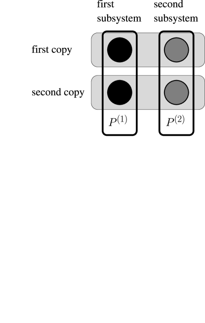
Figure 2: An expectation value $\langle\Psi|a|\Psi\rangle$ with respect to a single copy of a given state $|\Psi\rangle$ can not discriminate separable from entangled states. However, this is possible, if expectation values with respect to two copies are used. The grey boxes symbolise the two copies of the state $|\Psi\rangle$, with first subsystem (black) and second subsystem (grey). This scheme defines the structure of an operator acting on two copies of the single subsystems, such that the corresponding expectation values vanish exactly if the state $|\Psi\rangle$ is separable.

$$c(\Psi)=\sqrt{\bigl{.}\langle\Psi|\otimes\langle\Psi|\ A\ |\Psi\rangle\otimes|\Psi\rangle\bigr{.}}\ ,$$ (62)

where $A$ is acting on ${\cal H}\otimes{\cal H}$, i.e on ${\cal H}_{1}\otimes{\cal H}_{2}\otimes{\cal H}_{1}\otimes{\cal H}_{2}$. Of course, one needs to require that Eq. (62) vanishes for any separable state $|\Psi\rangle=|\varphi\rangle\otimes|\phi\rangle$. The simplest possibility could be an operator $A$ that decomposes into a part acting only on the copies of the first subsystem and a second part acting on the copies of the second subsystem. Not necessarily the unique, but a good choice for $A$ are projectors $P_{-}^{(k)}$ $(k=1,2)$ onto antisymmetric subspaces ${\cal H}_{-}^{k}$ of the space ${\cal H}_{k}\otimes{\cal H}_{k}$. They contain all states that acquire a phase shift of $\pi$ under the exchange of the two copies of $\cal H_{k}$. Thus, any state $|\psi_{-}\rangle\in{\cal H}_{-}^{k}$ can be expressed as $|\psi_{-}\rangle=\sum_{ij}\psi_{ij}(|ij\rangle-|ji\rangle)$, where the states $\{|i\rangle\}$ and $\{|j\rangle\}$ form an arbitrary basis of $\cal H_{k}$.

Indeed, since the two-fold copy $|\varphi\rangle\otimes|\varphi\rangle$ of a state is a symmetric object - it remains invariant under an exchange of the copies - the expectation value $\langle\varphi|\otimes\langle\varphi|P_{-}^{(1)}|\varphi\rangle\otimes|\varphi\rangle$ vanishes for any state $|\varphi\rangle\in{\cal H}_{1}$, and the same holds true for the analogous expression for ${\cal H}_{2}$.

Now, one can define $A:=4P_{a}$ in Eq. (62), with the projector $P_{a}$ onto the space spanned by the states in ${\cal H}_{1}\otimes{\cal H}_{2}\otimes{\cal H}_{1}\otimes{\cal H}_{2}$ that are antisymmetric both with respect to an exchange of the two copies of ${\cal H}_{1}$, and with respect to an exchange of the two copies of ${\cal H}_{2}$. The concurrence in Eq. (62) then necessarily vanishes for separable states. The prefactor $4$ is just a normalisation chosen such that the concurrence ranges from $0$ to $1$ for two-level systems. With this normalisation, the present definition is indeed equivalent to Eq. (59).

One may find it easier to interprete $A$ in terms of the two copies of the single subspaces ${\cal H}_{1}$ and ${\cal H}_{2}$. For this purpose, let’s identify ${\cal H}_{1}\otimes{\cal H}_{2}\otimes{\cal H}_{1}\otimes{\cal H}_{2}$ and ${\cal H}_{1}\otimes{\cal H}_{1}\otimes{\cal H}_{2}\otimes{\cal H}_{2}$. Then - as illustrated in Fig. 2 - $A$ is just the tensor product of the two projectors onto the two involved anti-symmetric subspaces:

$$A=4P_{-}^{(1)}\otimes P_{-}^{(2)}\ .$$ (63)

If a state $|\Psi\rangle$ is separable, the expectation value $\langle\Psi|\otimes\langle\Psi|A|\Psi\rangle\otimes|\Psi\rangle$ factorises into the product of the analogous expressions corresponding to the single subsystems

$$\langle\Psi|\otimes\langle\Psi|A|\Psi\rangle\otimes|\Psi\rangle=4\langle\varphi|\otimes\langle\varphi|P_{-}^{(1)}|\varphi\rangle\otimes|\varphi\rangle\langle\phi|\otimes\langle\phi|P_{-}^{(2)}|\phi\rangle\otimes|\phi\rangle\ ,$$ (64)

and vanishes because both, $|\varphi\rangle\otimes|\varphi\rangle$ and $|\phi\rangle\otimes|\phi\rangle$, are symmetric. However, for an entangled state $|\Psi\rangle=\sum_{i}\sqrt{\lambda_{i}}|\xi_{i}\rangle_{1}\otimes|\xi_{i}\rangle_{2}$ - for convenience represented in its Schmidt decomposition, Eq. (8) - the two-fold copy $|\Psi\rangle\otimes|\Psi\rangle$ is not symmetric under exchange of the copies of any of the subsystems. Thus, $|\Psi\rangle\otimes|\Psi\rangle$ necessarily has some anti-symmetric part, and the expectation value of $A$ with respect to this two-fold copy of $|\Psi\rangle$ is strictly positive.

Now, with this definition of $A$, one can also rephrase the concurrence of a mixed state $\varrho$ in terms of subnormalised states, Eq. (30), as

$$c(\varrho)=\inf_{\{|\psi_{i}\rangle\}}\sum_{i}\sqrt{\langle\psi_{i}|\otimes\langle\psi_{i}|\ A\ |\psi_{i}\rangle\otimes|\psi_{i}\rangle}\ .$$ (65)

If one makes use of the prescription (31) to characterise all decompositions of $\varrho$ into pure states, it reveals useful to define a tensor $\cal A$ that contains the elements of $A$ evaluated with the subnormalised states $\{|\phi_{j}\rangle\}$

$${\cal A}_{jk}^{lm}=\langle\phi_{l}|\otimes\langle\phi_{m}|\ A\ |\phi_{j}\rangle\otimes|\phi_{k}\rangle\ .$$ (66)

One can now easily rewrite $c(\varrho)$ in the closed expression

$$c(\varrho)=\inf_{V}\sum_{i}\sqrt{\bigl{[}V\otimes V\ {\cal A}\ V^{\dagger}\otimes V^{\dagger}\bigr{]}_{ii}^{ii}}\ ,$$ (67)

where the optimisation is to be performed over all left unitaries $V$.

2.3.1 Symmetries of $A$

We required $A$ to be anti-symmetric with respect to the exchange of the two copies of ${\cal H}_{1}$ as well as of ${\cal H}_{2}$. Though, this choice is not unique. It would have been sufficient to require only one of these symmetries. Here, we will briefly sketch the consequences of specific choice of $A$. In Section 2.3.2 and later on in Section 3, it will become apparent why it is of importance to require both symmetries.

With our above definition, Eq. (63), of $A$, the elements of $\cal A$

$${\cal A}_{jk}^{lm} = \mbox{Tr}\bigl{[}|\phi_{j}\rangle\langle\phi_{l}|\phi_{k}\rangle\langle\phi_{m}|\bigr{]}-\mbox{Tr}_{1}\Bigl{[}\mbox{Tr}_{2}\bigl{[}|\phi_{j}\rangle\langle\phi_{l}|\bigr{]}\mbox{Tr}_{2}\bigl{[}|\phi_{k}\rangle\langle\phi_{m}|\bigr{]}\Bigr{]}-$$ (68)

$$\mbox{Tr}_{2}\Bigl{[}\mbox{Tr}_{1}\bigl{[}|\phi_{j}\rangle\langle\phi_{l}|\bigr{]}\mbox{Tr}_{1}\bigl{[}|\phi_{k}\rangle\langle\phi_{m}|\bigr{]}\Bigr{]}+\mbox{Tr}\bigl{[}|\phi_{j}\rangle\langle\phi_{l}|\bigr{]}\mbox{Tr}\bigl{[}|\phi_{k}\rangle\langle\phi_{m}|\bigr{]}$$

contain partial traces over both subsystems, in a balanced way, what would not have been the case for other choices. E.g., for a projector ${\tilde{A}}$ onto the space spanned by all the states that are antisymmetric with respect only to the exchange of ${\cal H}_{1}$, the analogous expression reads

$$\tilde{\cal A}_{jk}^{lm}=2\left(\mbox{Tr}\bigl{[}|\phi_{j}\rangle\langle\phi_{l}|\phi_{k}\rangle\langle\phi_{m}|\bigr{]}-\mbox{Tr}_{1}\Bigl{[}\mbox{Tr}_{2}\bigl{[}|\phi_{j}\rangle\langle\phi_{l}|\bigr{]}\mbox{Tr}_{2}\bigl{[}|\phi_{k}\rangle\langle\phi_{m}|\bigr{]}\Bigr{]}\right)\ .$$ (69)

Whereas the symmetric treatment of both subsystems does not have any practical consequences, and is of rather aesthetical character, there is a much more crucial property: ${\cal A}$ is invariant under exchanges of the co- or contra-variant indices, ${\cal A}_{jk}^{lm}={\cal A}_{kj}^{lm}={\cal A}_{jk}^{ml}$. This symmetry will turn out to be the crucial ingredient required for the approximations to be discussed in Section 3.

2.3.2 Two-level systems

In the case of two-level systems, there is only one anti-symmetric state, namely $|01\rangle-|10\rangle$. Therefore, the projectors onto the anti-symmetric subspaces ${\cal H}_{-}^{1}$ and ${\cal H}_{-}^{2}$ have only one non-vanishing eigenvalue. This, in turn, also holds true for $A$ which reads $A=|\chi\rangle\langle\chi|$, with

$$|\chi\rangle=|0011\rangle-|0110\rangle-|1001\rangle+|1100\rangle\ .$$ (70)

Consequently, ${\cal A}$ can be expanded in terms of a single matrix $\tau$ as

$${\cal A}_{jk}^{lm}=\tau_{lm}^{\ast}\tau_{jk}\ ,\hskip 14.22636pt\mbox{with}\hskip 14.22636pt\tau_{jk}=\langle{\chi}|{\phi_{j}}\rangle\otimes|{\phi_{k}}\rangle\ .$$ (71)

Due to the symmetry of $A$ discussed above in Section 2.3.1, $\tau$ is indeed symmetric, i.e. satisfies a crucial precondition for the generalisation to mixed states. Expressed in terms of $\tau$, Eq. (67) now simplifies to

$$c(\varrho)=\inf_{V}\sum_{i}\sqrt{\left[V^{\ast}\tau^{\ast}V^{\dagger}\right]_{ii}\left[V\tau V^{T}\right]_{ii}}=\inf_{V}\sum_{i}\left|\left[V\tau V^{T}\right]_{ii}\right|\ .$$ (72)

Due to the symmetry of $\tau$, the infimum is exactly given in terms of the singular values of $\tau$, as discussed in the context of Eq. (38).

The relation between the present and the original approach to concurrence [27, 57] becomes apparent with the observation that the matrix $\tau$ defined here coincides with that introduced in Eq. (38)

$$\tau_{jk}=\langle{\chi}|{\phi_{j}}\rangle\otimes|{\phi_{k}}\rangle=\langle\phi_{j}^{\ast}|\sigma_{y}\otimes\sigma_{y}|\phi_{k}\rangle\ ,$$ (73)

in the $2\times 2$ case. Thus, the original approach to concurrence is naturally embedded in the present, more general framework.

2.3.3 Higher dimensional systems

The formalism in terms of projectors onto anti-symmetric subspaces can also be used to formulate a generalisation of concurrence to systems of arbitrary dimensions. For an $n_{1}\times n_{2}$-dimensional system, $A$ has $m=n_{1}(n_{1}-1)n_{2}(n_{2}-1)/4$ non-vanishing eigenvalues - $n_{1}(n_{1}-1)/2$ corresponding to the antisymmetric subspace of ${\cal H}_{1}\otimes{\cal H}_{1}$, and analogously for ${\cal H}_{2}\otimes{\cal H}_{2}$. Thus, $A$ cannot be expressed with the help of a single eigenvector anymore, but with a finite sum

$$A=\sum_{\alpha=1}^{m}|\chi_{\alpha}\rangle\langle\chi_{\alpha}|\ ,$$ (74)

which contains $n_{1}(n_{1}-1)n_{2}(n_{2}-1)/4$ non-vanishing terms. Due to the symmetries ${\cal A}_{jk}^{lm}={\cal A}_{kj}^{lm}={\cal A}_{jk}^{ml}$ which we already observed in Section 2.3.1, all $T^{\alpha}$ with the elements

$$T_{jk}^{\alpha}=\langle{\chi_{\alpha}}|{\phi_{j}}\rangle\otimes|{\phi_{k}}\rangle\ ,\alpha=1,\ldots,m=n_{1}(n_{1}-1)n_{2}(n_{2}-1)/4\ ,$$ (75)

are symmetric. Furthermore, the eigenvectors of $A$ still carry an undetermined phase factor $e^{i\varphi_{\alpha}}$. Whereas these free phases usually do not matter, they provide an additional freedom which we shall exploit in Section 3. Therefore, we explicitly account for the free phases $\varphi_{\alpha}$, and Eq. (67) consequently reads

$$c(\varrho)=\inf_{V}\sum_{i}\sqrt{\sum_{\alpha}\left|\left[VT^{\alpha}e^{i\varphi_{\alpha}}V^{T}\right]_{ii}\right|^{2}}\ .$$ (76)

There are two crucial differences as compared to Eq. (72) that hamper finding the exact infimum: First, the square and the square root in Eq. (76) lead to non-linear expressions in the $T^{\alpha}$, and, second, the already mentioned fact that the several distinct symmetric matrices $T^{\alpha}$ cannot, in general, be diagonalised simultaneously.

One of the earliest generalisations of concurrence to higher dimensional systems that does not lead to the non-linear behaviour, as it appears in Eq. (76), is the concurrence vector. Although the original definition [64] is slightly different, we will describe it here in terms of the projectors of Eq. (63), in order to highlight the similarities with our own approach. Each $|\chi_{\alpha}\rangle$ inherits a negative pre-factor under the exchange of the two copies of either ${\cal H}_{1}$ or ${\cal H}_{2}$. The product $|\Psi_{s}\rangle\otimes|\Psi_{s}\rangle$ of an arbitrary separable state is invariant under such transformations. Since the overlap

$${\cal C}_{\alpha}(\Psi)=\langle{\chi_{\alpha}}|{\Psi}\rangle\otimes|{\Psi}\rangle$$ (77)

is invariant under the exchange of the two copies, it necessarily needs to vanish for any $|\chi_{\alpha}\rangle$ and any separable state $|\Psi\rangle=|\Psi_{s}\rangle\otimes|\Psi_{s}\rangle$. In contrast, whenever ${\cal C}_{\alpha}(\Psi)$ is positive, the state $|\Psi\rangle$ necessarily needs to be entangled. The inverse implication is a bit more involved - $|\Psi\rangle$ is separable, if ${\cal C}_{\alpha}(\Psi)=0$, for $\alpha=1,\ldots,n_{1}(n_{1}-1)n_{2}(n_{2}-1)/4$.

The generalisation of the above for mixed states is now straightforward and analogous to the case of two-level systems discussed in Section 2.3.2. A given state $\varrho$ is separable if and only if there is a left-unitary transformation $V$ such that all elements

$${\cal C}_{\alpha}=\sum_{j}\left|\left[VT^{\alpha}V^{T}\right]_{jj}\right|\ ,$$ (78)

of the concurrence vector ${\cal C}$ vanish. However, this – necessary and sufficient – separability criterion is, in general, difficult to evaluate – since, again, in general the matrices $T^{\alpha}$ cannot be diagonalised simultaneously. Nevertheless, it establishes the basis for some operational, though only necessary separability criteria. It implies that a given state is entangled if the singular values ${\cal S}_{j}^{({\alpha})}$ of one matrix $T^{\alpha}$ satisfy ${\cal S}_{1}^{({\alpha})}-\sum_{j}{\cal S}_{j}^{({\alpha})}>0$. Another – in general stronger – criterion is obtained with the help of linear combinations $\sum_{\alpha}z_{\alpha}T^{\alpha}$ of all matrices $T^{\alpha}$, with complex pre-factors $z_{\alpha}$. For a suitably chosen set $\{z_{\alpha}\}$, the expression ${\cal S}_{1}-\sum_{j}{\cal S}_{j}$ can be significantly larger than the corresponding expression for a single matrix $T^{\alpha}$ [64].

Concurrence vector is not a measure and as such does not provide an adequate tool for our aims, i.e. the quantitative characterisation of temporally evolving entanglement. Though, in section 3 we will show that - despite its non-linearity - Eq. (76) can be used to derive some means for such a quantification.

2.3.4 Gradient

Before we focus on this, however, let’s discuss how to assess concurrence numerically. As mentioned in Section 1.4.2, the cardinality of the ensemble that realises the infimum in Eq. (29) can exceed the rank $r(\varrho)$, though is bounded by $r^{2}(\varrho)$ [52]. This is the cause of the appearance of a rectangular, left-unitary matrix $V$ instead of a quadratic, unitary matrix $U$ in Eq. (67). In the present section, however, matrices of the latter type are more convenient. Therefore, we will fix the cardinality of the considered ensembles. If it turns out that the assumed cardinality is not large enough, one can always increase it by adding some null-vectors to the ensemble.

According to Eq. (67), the concurrence of a mixed state $\varrho$ is given by

$$c(\varrho)=\inf_{U}{\cal C}(U)\ ,\hskip 14.22636pt\mbox{with}\hskip 14.22636pt{\cal C}(U)=\sum_{i}\sqrt{\left[U\otimes U{\cal A}\ U^{\dagger}\otimes U^{\dagger}\right]_{ii}^{ii}}\ .$$ (79)

If one considers an infinitesimal transformation $dU={\mathbbm{1}}+i\epsilon K$ , with $\epsilon$ infinitesimally small, and uses the symmetry of ${\cal A}$ with respect to an exchange of co- and contravariant indices, this can be written as

$${\cal C}(dU)\simeq\sum_{i}\sqrt{A_{ii}^{ii}}+\frac{i\epsilon}{\sqrt{A_{ii}^{ii}}}\left[K\otimes{\mathbbm{1}}\ A\ -A\ K\otimes{\mathbbm{1}}\right]_{ii}^{ii}\ ,$$ (80)

where the expansion $\sqrt{a+\varepsilon}\simeq\sqrt{a}+\varepsilon/(2\sqrt{a})$ of the square root function was employed. This allows to rephrase ${\cal C}(dU)$ as

$${\cal C}(dU)=\sum_{i}\sqrt{A_{ii}^{ii}}+\varepsilon\ \sum_{ij}K_{ij}G_{ji}\ ,\hskip 14.22636pt\mbox{with}\hskip 14.22636ptG_{ji}=i\left(\frac{A_{ji}^{ii}}{\sqrt{\big{.}A_{ii}^{ii}}}-\frac{A_{jj}^{ij}}{\sqrt{A_{jj}^{jj}}}\right)\ .$$ (81)

Since the square root is not analytic in the origin, one has to take care that $A_{ii}^{ii}$ be non-vanishing for all $i$. This is the case if and only if there are only non-separable pure states $|\Psi_{i}\rangle$ in the decomposition of $\varrho$, since, by Eq. (62) and Eq. (66), the elements $A_{ii}^{ii}$ are the squares of the concurrences of the states $|\Psi_{i}\rangle$. Though, even if the denominators in Eq. (81) vanish, the numerators behave accordingly [68], such that Eq. (81) is indeed always well defined.

The hermitian matrix $G$ in Eq. (81) can be considered as a gradient, since the increment of ${\cal C}$ reads

$${\cal C}(dU)-{\cal C}({\mathbbm{1}})=\varepsilon\ \mbox{Tr}\left[KG\right]\ ,$$ (82)

what is just a Hilbert-Schmidt scalar product [35]. Accordingly, the direction of steepest descent of $\cal C$ is given by $-G$. Minima of ${\cal C}$ can therefore be found by repeated application of the transformation $dU=\exp(-i\epsilon G)$. However, also more refined methods can be used, such as the conjugate-gradient minimisation [64, 69]. In this method, the iteration is not performed exactly along the current gradient $G_{n}$, but it takes into account corrections that ensure that the previous iteration along the gradient $G_{n}$ is not reversed. More explicitely the iteration is performed along

$$\tilde{G}_{n}=G_{i}-\gamma G_{n-1}\ , \gamma=\frac{\mbox{Tr}\left[\left(G_{n}-\tau G_{n-1}\right)G_{n}\right]}{\mbox{Tr}\left[G_{n-1}^{2}\right]}\ ,$$ with (83)

and $$\tau G_{n-1}=e^{i\frac{\varepsilon}{2}\tilde{G}_{n-1}}G_{n-1}e^{-i\frac{\varepsilon}{2}\tilde{G}_{n-1}}\ .$$

However, there is in general no a priori information available on whether the solution reached by that procedure is a local or a global minimum. While one may start the iteration with different initial conditions parametrised by $U$, in order to get a better intuition on the effective “landscape” defining the optimisation problem at hand, this uncertainty persists, and the more so the higher the dimension of the parameter space over which the optimisation is carried out.

2.3.5 Multi-partite systems

Since lately several experimental groups [7, 8, 9, 10, 11, 12, 13, 14] systematically investigate quantum correlations in multipartite systems, i.e., systems with more than two subsystems, a quantitative description of multipartite entanglement is highly desirable. Multipartite systems keep room for distinct classes of quantum states: Even for a pure state $|\Psi\rangle$ of a tri-partite two-level system more than a single scalar quantity is required for complete characterisation of all inscribed quantum correlations.

In bipartite systems, any state can be prepared using LOCC only, starting with a distinguished, maximally entangled state (see Section 1.4.1). This is no longer true in multipartite systems - where inequivalent kinds of multipartite entanglement exist [70]. Consider for example a Greenberger-Horne-Zeilinger state (GHZ-state) [22]

$$|\Psi_{\rm{GHZ}}\rangle=\frac{1}{\sqrt{2}}\bigl{(}|000\rangle+|111\rangle\bigr{)}\ ,$$ (84)

and a W-state [70]

$$|\Psi_{\rm{W}}\rangle=\frac{1}{\sqrt{3}}\bigl{(}|001\rangle+|010\rangle+|100\rangle\bigr{)}\ .$$ (85)

Both states contain fundamentally different correlations, such that none of the two can be created from the other one by LOCC alone [70]. Thus, one cannot expect that a single scalar quantity can completely describe $p$-particle correlations (with $p>2$).

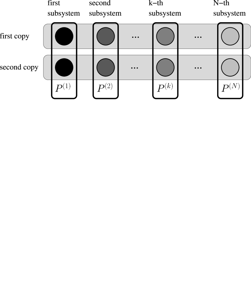
Figure 3: The concurrence of bipartite states is defined in terms of two operators, each of which is associated with two copies of one subsystems, as displayed in Fig. 2. This concept can straightforwardly be generalised to multipartite systems. For each two copies of one subsystems, there is one operator $P^{(k)}$.

Hence, how can we generalise the concept of concurrence to multipartite systems? The definition of concurrence in Eq. (59) is not very suggestive for generalisations: While the degree of mixing of the reduced density matrix has an unambiguous interpretation for bipartite systems, its meaning is unclear in the multipartite case. Though, Eq. (62) has a rather obvious multipartite formulation, what implies a generalisation of concurrence for multipartite systems that can describe at least some of the correlations we are seeking for. A generalisation of concurrence [71] for tri-partite two-level systems is already available – it characterises all tri-partite correlations of pure states. In the following, we present an even more general framework applicable to systems with an arbitrary number of subsystems, for pure and mixed states.

Similarly to the case of bipartite concurrence, also its multipartite generalisations can be defined in terms of an operator $A$ acting on the tensor product of ${\cal H}$ with itself. The only difference being that ${\cal H}$ is the tensor product of more than two factor spaces ${\cal H}_{i}$. Any tensor product of projectors onto symmetric and anti-symmetric sub-spaces is positive semi-definite, and invariant under local unitary transformations, see Fig. 3. However, not all such operators finally lead to tensors ${\cal A}$ with the desired invariance under exchange of co- or contravariant indices. This symmetry is only valid for products of an even number of projectors $P_{-}^{(i)}$ onto anti-symmetric subspaces, possibly multiplied with some projectors $P_{+}^{(i)}$ onto symmetric subspaces. On the other hand, all expectation values of the type appearing on the right hand side of Eq. (62), with $A$ a product of an odd number of projectors onto anti-symmetric subspaces, vanish anyway, for arbitrary states.

Thus, we define $N$-partite concurrence as in Eq. (62), i.e.

$$c(\Psi)=\sqrt{\bigl{.}\langle\Psi|\otimes\langle\Psi|\ A\ |\Psi\rangle\otimes|\Psi\rangle\bigr{.}}\ ,$$ (86)

in terms of a sum of direct products of projectors onto symmetric and anti-symmetric subspaces

$$A=\sum_{{\cal V}{\{s_{i}=\pm\}}\atop{\prod_{i=1}^{N}s_{i}=+}}p_{\{s_{i}\}}\bigotimes_{j=1}^{N}P_{s_{j}}^{(j)}\ ,\ p_{\{s_{i}\}}\geq 0\ .$$ (87)

Here, ${\cal V}{\{s_{i}=\pm\}}$ represents all possible variations of an $N$-string of the symbols $+$ and $-$, and the summation is restricted to contributions with an even number of projectors onto anti-symmetric subspaces.

Note that, because of the continuous parametrisation in terms of the $p_{\{s_{i}\}}$, Eq. (87) actually defines a continuous family of multipartite concurrences. While the intuitive interpretation of the concurrence defined by an arbitrary choice of the $p_{\{s_{i}\}}$ so far remains an open problem, there are some specific choices of the $p_{\{s_{i}\}}$ that have immediate applications in the characterisation of the multipartite entangled states dealt with in Section 4. Let’s take all prefactors $p_{\{s_{i}\}}$ in Eq. (87) equal, with the only exception of setting $p_{+\ldots+}=0$. As in Eq. (63), there is some freedom in the normalisation. Once again we set $p_{\{s_{i}\}}=4$ - just to be consistent with Eq. (63). The concurrence $c_{N}$, defined with these prefactors for systems with an arbitrary number $N$ of subsystems, can be expressed in terms of the reduced density matrices $\varrho_{i}$  [32] as

$$c_{N}(\Psi)=2^{1-\frac{N}{2}}\sqrt{(2^{N}-2)\langle\Psi|\Psi\rangle^{2}-\sum_{i}\mbox{Tr}\varrho_{i}^{2}}\ .$$ (88)

The index $i$ runs over all $(2^{N}-2)$ nontrivial subsets of an $N$-particle system. Obviously, $c_{N}$ vanishes only for completely separable $N$-particle states, since all reduced density matrices are simultaneously pure only for these states. What is less obvious but at least equally important is that $c_{N}$ allows to compare the entanglement of $N$- and $(N-1)$-partite states: for any state $|\Psi\rangle$ that factorises into a product of a one-particle state and a $(N-1)$-partite remainder $|\varPhi\rangle$, $c_{N}(\Psi)$ reduces to $c_{N\mbox{-}1}(\varPhi)$. Thus, $c_{N}$ is perfectly suited to investigate the scaling properties of multipartite entanglement with the system size $N$, what we shall explore in Section 4.2.3.

Further entanglement-properties can be addressed by other choices of the $p_{\{s_{i}\}}$ in Eq. (87): for example, bi-separability of tri-partite states can be characterised by $c_{3}^{(23)}$, with $A_{3}^{(23)}=4P_{+}^{(1)}\otimes P_{-}^{(2)}\otimes P_{-}^{(3)}$, and, analogously, by $c_{3}^{(13)}$, with ${A}_{3}^{(13)}=4P_{-}^{(1)}\otimes P_{+}^{(2)}\otimes P_{-}^{(3)}$, or by $c_{3}^{(12)}$, with ${A}_{3}^{(12)}=4P_{-}^{(1)}\otimes P_{-}^{(2)}\otimes P_{+}^{(3)}$. The subscript represents the number of subsystems as in Eq. (88) while the superscript stands for the subsets in which quantum correlations are measured. Consider $|\Psi\rangle=|\varPhi_{12}\rangle\otimes|\varphi_{3}\rangle$ as an exemplary state. The choice $c_{3}^{(12)}$ quantifies the bipartite concurrence of the entangled part $|\varPhi_{12}\rangle$ of $|\Psi\rangle$, i.e., $c_{3}^{(12)}(\Psi)=c(\varPhi_{12})$, whereas $c^{(23)}_{3}$ and $c^{(13)}_{3}$ vanish identically for this bi-separable state. This selectivity with respect to correlations between specific subgroups of subsystems also hold for bi-separable mixed states - guaranteed by the construction (29) as convex roof.

Another interesting quantity emerges for four-partite systems: Since the number of subsystems is even, there is a term ${A}_{4}^{(1234)}=4P_{-}^{(1)}\otimes P_{-}^{(2)}\otimes P_{-}^{(3)}\otimes P_{-}^{(4)}$ that does not contain any factor $P_{+}^{(i)}$. The corresponding concurrence vanishes for all states that do not contain proper four-partite correlations, i.e., bi-separable and tri-separable states. In particular, for a GHZ state, $c_{4}^{(1234)}(\Psi_{\rm GHZ})=2\sqrt{\sum_{i\neq j}\lambda_{i}\lambda_{j}}$ while $c_{4}^{(1234)}$ vanishes for $W$-states – similarly like for tri-partite systems where $W$-states bear only bipartite correlations . In the specific case of two-level systems, this particular choice of $c_{4}^{(1234)}$ measures the potential of a given state for multi-particle teleportation [72].

3 Lower bounds

In the case of bipartite two-level systems, we were able to evaluate the concurrence of arbitrary mixed states $\varrho$ exactly. This was possible because ${\cal A}$ (see Eq. (66)) was of rank one. For higher dimensional systems ${\cal A}$ typically is of higher rank, such that Eq. (76) exhibits two complications with respect to Eq. (72): additional non-linearities, and different matrices $T^{\alpha}$ which, in general, cannot be diagonalised simultaneously. These two properties have so far prevented the derivation of an explicit solution of the optimisation problem formulated in Eq. (76). However, as we will show now, concurrence can be bounded from below, by some suitable approximations [30, 31].

First, the Cauchy-Schwarz inequality [73]

$$\Bigl{(}\sum_{\alpha}x_{\alpha}^{2}\Bigr{)}^{\frac{1}{2}}\Bigl{(}\sum_{\alpha}y_{\alpha}^{2}\Bigr{)}^{\frac{1}{2}}\geq\sum_{\alpha}x_{\alpha}y_{\alpha}$$ (89)

allows to linearise Eq. (76). With $x_{\alpha}:=\left|\bigl{[}VT^{\alpha}e^{i\varphi_{\alpha}}V^{T}\bigr{]}_{ii}\right|$, we conclude that

$$c(\varrho)\geq\inf_{V}\sum_{i=1}^{N}\sum_{\alpha=1}^{m}y_{\alpha}\left|\Bigl{[}VT^{\alpha}e^{i\varphi_{\alpha}}V^{T}\Bigr{]}_{ii}\right|,\hskip 14.22636pt\mbox{with}\hskip 14.22636pt\sum_{\alpha}y_{\alpha}^{2}=1\ ,$$ (90)

where we introduced some auxiliary real parameters $y_{\alpha}$. However, the different matrices $T^{\alpha}$ still cause trouble finding the desired infimum. Here, the triangle inequality

$$\sum_{\alpha}\bigl{|}z_{\alpha}\bigl{|}\geq\bigl{|}\sum_{\alpha}z_{\alpha}\bigl{|}\ ,$$ (91)

valid for arbitrary complex numbers $z_{\alpha}$, allows to circumvent this problem: For $z_{\alpha}:=y_{\alpha}\bigl{[}VT^{\alpha}e^{i\varphi_{\alpha}}V^{T}\bigr{]}_{ii}$, and $y_{\alpha}\geq 0$, one obtains

$$c(\varrho)\geq\inf_{V}\sum_{i=1}^{N}\left|\Bigl{[}V\Bigl{(}\sum_{\alpha=1}^{m}y_{\alpha}T^{\alpha}e^{i\varphi_{\alpha}}\Bigr{)}V^{T}\Bigr{]}_{ii}\right|\ ,$$ (92)

an expression for which the infimum is given analytically by Eq. (44). Our final expression for a lower bound of the concurrence therefore reads

$$c(\varrho)\geq\max\left\{{\cal S}_{1}-\sum_{i>1}{\cal S}_{i},\ 0\right\}\ ,$$ (93)

with the singular values ${\cal S}_{j}$ of

$${\cal T}=\sum_{\alpha}Z_{\alpha}T^{\alpha},\ Z_{\alpha}=y_{\alpha}e^{i\varphi_{\alpha}},\ {\rm and}\ {\sum_{\alpha}|Z_{\alpha}|^{2}=1}\ .$$ (94)

The bound in Eq. (93) still depends on the choice of the $Z_{\alpha}$, what allows to tighten the estimate. Thus, one is left with an optimisation problem on an $2m$-dimensional parameter space [30], where $m$ is the number of matrices $T^{\alpha}$ in Eq. (75). Note that the constraint $\sum_{\alpha}|Z_{\alpha}|^{2}=1$ is by far simpler to implement than left unitarity, Eq. (31), since it is easily parametrised. Moreover, the dimension $m$ of optimisation space is significantly reduced as compared to the dimension $n_{1}^{3}n_{2}^{3}$ of the original optimisation problem defined by Eqs. (29) and (31).

3.1 Purely algebraic bounds

The lower bound of Eq. (92) was obtained by the replacement of several matrices $T^{\alpha}$ by a single suitably chosen ${\cal T}=\sum_{\alpha}Z_{\alpha}T^{\alpha}$. So far, there is no clear prescription of how to chose the expansion coefficients $Z_{\alpha}$, which is partially due to the fact that the $T^{\alpha}$ are determined only up to degeneracy. They are constructed with the help of the eigenvectors $|\chi_{\alpha}\rangle$ of the projector $A$, what specifies an eigenspace, but does not distinguish states within these subspaces.

One way to get rid of this ambiguity is to diagonalise ${\cal A}$ instead of $A$. For a typical state $\varrho$, ${\cal A}$ will have no degenerate eigenvalues, and thus has uniquely defined eigenvectors $T^{\alpha}$. One can then provide $m$ different lower bounds of concurrence directly calculating the singular values ${\cal S}_{j}$ in Eq. (93) for

$${\cal T}=T^{\alpha},\ \alpha=1,\ldots m.$$ (95)

In Section 3.3 we will see that one of these bounds alone may already yield a satisfactory approximation to the optimised lower bound.

3.2 Quasi-pure approximation

By now, a large number of experiments focusses on the (controlled) preparation and evolution of entangled states. Any degree of mixing - i.e. , the presence of classical correlations – decreases quantum correlations, and can lead to their complete destruction. Therefore – in particular in view of the many potential technical applications of non-classically correlated quantum states – pure entangled states are the experimentalist’s desire: hence it is crucial to screen the investigated systems from the environment.

In general, perfect screening is impossible, but experimental techniques are sufficiently advanced [5, 8, 74] to preserve entanglement over appreciable periods of time. Yet, very little is known on the precise temporal evolution of such states even under weak but finite environment coupling, one of the principal obstacles being the lack of computable entanglement measures for arbitrary states.

On the other hand, a general quantifier for entanglement, applicable to arbittrary states, is not even needed in this context, since environmental influences can be assumed to be small under the given experimental conditions. Indeed the evolution of an initially pure into a mixed state occurs on a rather long time scale, and the experimentally interesting states are - though not exactly pure - at least quasi-pure, i.e. , they have one single eigenvalue $\mu_{1}$ that is much larger than all the other ones.

In order to provide some efficient means to deal with this type of problems, we now derive an analytic approximation of concurrence for quasi-pure states [31]. Indeed, we will find that this approximation also leads to a lower bound for arbitrary states. This quasi-pure approximation will allow for an efficient quantitative treatment of non-classical correlations that arise in most present day experiments.

The matrix ${\cal A}$ defined in Eq. (66) contains the matrix elements of $A$ evaluated with the subnormalised (see Eq. (30)) eigenstates of $\varrho$. Therefore, the elements of ${\cal A}$ are proportional to the eigenvalues $\mu_{i}$ of the considered state:

$${\cal A}_{jk}^{lm}\sim\sqrt{\bigl{.}\mu_{j}\mu_{k}\mu_{l}\mu_{m}\bigr{.}}\ .$$ (96)

Consequently, we can classify the elements of ${\cal A}$ according to their relative magnitude determined by the eigenvalues $\mu_{j}$. This classification will serve as a basis for the approximate evaluation of concurrence in our subsequent treatment.

The above proportionality leads to a natural order of the elements of ${\cal A}$, in terms of powers of square roots of the real eigenvalues $\mu_{i}$ of $\varrho$, which we assume to be labeled in decreasing order, i.e. , $\mu_{1}\gg\mu_{2}\geq\ldots\geq\mu_{n}$. Hence, if we consider terms proportional to either one of the $\mu_{j}$, with $j>1$, as perturbations of the dominant term ${\cal A}_{11}^{11}\sim\mu_{1}^{2}$, we obtain the following classification:

• the element ${\cal A}_{11}^{11}$ is lowest order,

• all elements with one index $j>1$, i.e. ${\cal A}_{j1}^{11}$, ${\cal A}_{1j}^{11}$, ${\cal A}_{11}^{j1}$ and ${\cal A}_{11}^{1j}$, are first order, and

• elements with two indices $j,k>1$, alike ${\cal A}_{jk}^{11}$ or ${\cal A}_{j1}^{k1}$, are second order.

However, this classification is not yet a sufficient basis for our approximation. In fact, the element ${\cal A}_{11}^{11}$ is lowest order, though still it could vanish. This is the case if and only if the subnormalised eigenstate $|\psi_{1}\rangle$ to the largest eigenvalue $\mu_{1}$ of $\varrho$ is separable, since $A_{11}^{11}$ is the square of the concurrence of $|\psi_{1}\rangle$ - see Eqs. (62) and (66). Therefore, as an additional requirement to quasi-purity we have to impose that $|\psi_{1}\rangle$ is entangled. Since the desired approximation is supposed to be applied to states that occur in the experiments mentioned above, this is not too stringent a restriction - if an ideal experiment without any environment coupling led to a pure state with non-negligible entanglement, it is reasonable to assume that the eigenstate $|\psi_{1}\rangle$ associated with the largest eigenvalue $\mu_{1}$ of $\varrho$ is not separable either.

We wish to approximate ${\cal A}$ by a matrix product

$${\cal A}_{jk}^{lm}\simeq{\cal T}_{lm}^{\ast}{\cal T}_{jk}\ ,$$ (97)

with a complex symmetric matrix ${\cal T}\in{\mathbbm{C}}^{n\times n}$. Such a replacement allows for an analytic solution, since the sum over $\alpha$ in Eq. (76) reduces to a single term, and the analytic expression Eq. (39) for the infimum, derived in Section 2.1, can be employed.

Specifically for the lowest order term ${\cal A}_{11}^{11}$, Eq. (97) yields ${\cal T}_{11}=\sqrt{{\cal A}_{11}^{11}}$, up to an arbitrary phase which can be dropped. Subsequently, evaluation of Eq. (97) for the first order elements leads to ${\cal T}_{j1}={\cal A}_{j1}^{11}/\sqrt{{\cal A}_{11}^{11}}$, employing also the expression for ${\cal T}_{11}$. Finally, we still have the freedom to fix ${\cal T}_{jk}$, for $j,k\neq 1$. For this purpose we use Eq. (97) for ${\cal A}_{jk}^{11}$, what leads to ${\cal T}_{jk}={\cal A}_{jk}^{11}/\sqrt{{\cal A}_{11}^{11}}$, such that all matrix elements of $\cal T$ are given by

$${\cal T}_{jk}=\frac{{\cal A}_{jk}^{11}}{\sqrt{{\cal A}_{11}^{11}}}\ .$$ (98)

With this choice of $\cal T$, Eq. (97) is exact at lowest and first order, and - in addition - the second order elements ${\cal A}_{jk}^{11}$ are taken into account correctly. Note that, using only one single matrix ${\cal T}$, it is not possible to describe accurately all second order elements, such as ${\cal A}_{j1}^{k1}$. All terms of third and fourth order are dropped in the present approximation.

Since we were assuming $|\psi_{1}\rangle$ to be entangled, i.e. , ${\cal A}_{11}^{11}$ finite by virtue of Eq. (62), ${\cal T}$ is well defined. Approximating ${\cal A}$ in terms of this matrix ${\cal T}$, Eq. (76) can be approximated as

$$c(\varrho)\simeq c_{\rm{qp}}(\varrho)=\inf_{V}\sum_{i}\left|\left[V{\cal T}V^{T}\right]_{ii}\right|\ ,$$ (99)

following the same steps as in the derivation of Eq. (72). As formulated in Eq. (44), the infimum can be expressed in terms of the decreasingly ordered singular values ${\cal S}_{i}$ of ${\cal T}$,

$$c_{\rm{qp}}(\varrho)=\max\left\{{\cal S}_{1}-\sum_{i>1}{\cal S}_{i},\ 0\right\}\ .$$ (100)

A priori, it is not clear up to which degree of mixing the quasi-pure approximation provides reliable estimates. The fact that not all second order elements are taken into account may somewhat reduce our confidence in a wide range of applicability for this approximation. However, we will see in Sections 4.1, 4.2.3, and 4.2.4 that the above ansatz provides very good results for many states, even for those with a substantial degree of mixing.

Indeed, the quasi-pure approximation is not only an approximation, but even a lower bound of concurrence: Given the decomposition ${\cal A}_{jk}^{lm}=\sum_{\alpha}(T_{lm}^{\alpha})^{\ast}T_{jk}^{\alpha}$, ${\cal T}$ is easily expressed as

$${\cal T}=\sum_{\alpha}z_{\alpha}T^{\alpha}\ ,\hskip 14.22636pt\mbox{with}\hskip 14.22636ptz_{\alpha}=\frac{\left(T_{11}^{\alpha}\right)^{\ast}}{\sqrt{\sum_{\beta}|T_{11}^{\beta}|^{2}}}\ .$$ (101)

Thus, ${\cal T}$ is indeed a valid symmetric matrix to provide a lower bound as formulated in Eq. (92).

3.3 Lower bounds of states with positive partial transpose

In the preceding section we collected a set of operational tools to access the non-classical correlations of arbitrary mixed quantum states of finite dimension - characterised by their concurrence. Our formal treatment spans the entire range from an approximation-free description for numerical implementation, over lower bounds that can be tightened numerically, to an easily tractable, purely algebraic estimate of the degree of entanglement of a quasi-pure quantum state which is typically dealt with in experiments. However, our approach is largely based on physical intuition, and so far we cannot come up with mathematically precise error bounds. Often, however, the latter are available in full mathematical rigour only under rather restrictive assumptions - while we are seeking for robust quantities which, beyond formal consistency, can cope with requirements which stem from real-world experiments.

Now we will test our toolbox under realistic conditions, and we start out with the detection of nonseparable states with positive partial transpose (ppt). In the next chapter, we will then use our approach to monitor the time evolution of entanglement, under various scenarios.

3.3.1 Some exemplary ppt states

One of the main requirements imposed on an entanglement measure is that it be able to distinguish entangled states from separable ones. Whereas a large class of entangled states is detected by the ppt criterion defined in Eq. (12), no operational criterion is known so far that can detect all states with positive partial transpose. In general it tends to be rather demanding to decide whether such states are entangled or not. Therefore - albeit our bound, Eq. (92), is capable of more than just checking separability - we use it, as a first test of its pertinence, as a separability criterion for some families of entangled states with positive partial transpose [39, 40, 75].

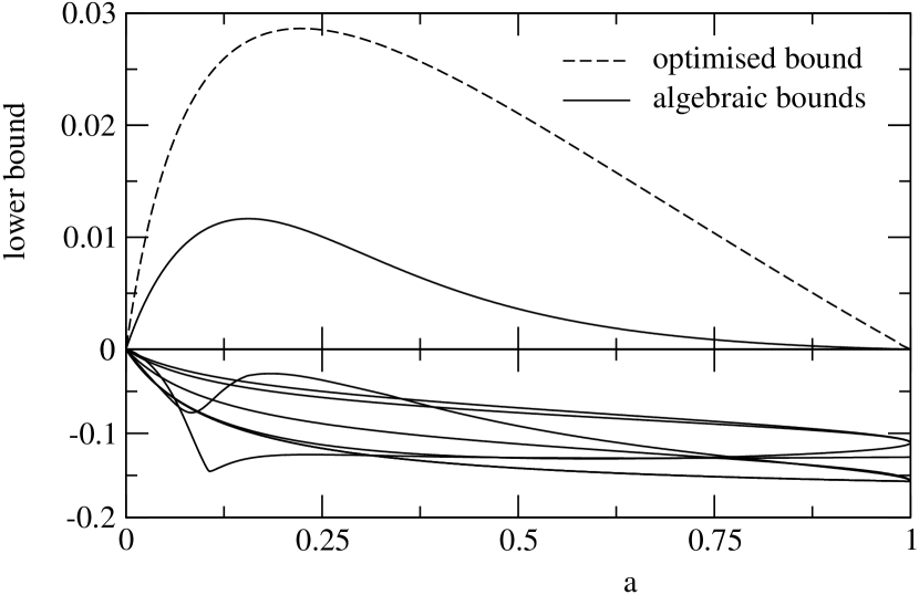
Figure 4: Numerically optimised lower bound (dashed line, Eqs. (93) and (94)) of the concurrence of the family of bipartite spin-1 states $\varrho_{a}$  [75] as defined in Eq. (102), together with the algebraic bounds (solid lines) obtained from Eq. (93) using (95). Both the optimised bound and the largest algebraic bound are positive, such that the state is detected as entangled in the entire parameter range $a=[0,1]$. All other algebraic lower bounds are negative. Note that the scale of concurrence (y-axis) is different for positive and negative bounds.

The first class of states describes a bipartite spin-$1$ system. The state $\varrho_{a}$ acting on ${\mathbbm{C}}^{3}\otimes{\mathbbm{C}}^{3}$ is given [39, 75], for $a\in[0,1]$, as

$$\varrho_{a}=\frac{1}{1+8a}\left[{\begin{array}[]{ccccccccc}a&0&0&0&a&0&0&0&a\\ 0&a&0&0&0&0&0&0&0\\ 0&0&a&0&0&0&0&0&0\\ 0&0&0&a&0&0&0&0&0\\ a&0&0&0&a&0&0&0&a\\ 0&0&0&0&0&a&0&0&0\\ 0&0&0&0&0&0&\beta&0&\gamma\\ 0&0&0&0&0&0&0&a&0\\ a&0&0&0&a&0&\gamma&0&\beta\end{array}}\right],\hskip 14.22636pt\mbox{with}\hskip 14.22636pt\left\{\begin{array}[]{l}\displaystyle\beta=\frac{1+a}{2}\ ,\\ \left.\right.\\ \displaystyle\gamma=\frac{\sqrt{1-a^{2}}}{2}\ ,\end{array}\right.$$ (102)

and has a positive partial transpose as defined in Eq. (12), in the entire range of $a$. The algebraic lower bounds defined by Eqs. (93) and (95) are plotted in Fig. 4 as solid lines. One of them is positive for all values of the parameter $a$, and the non-separability of $\varrho_{a}$ is therefore detected by a purely algebraic criterion. All other algebraic bounds are negative, and therefore do not provide any information on their own.

The dashed line in Fig. 4 shows the lower bound that is numerically optimised over the $Z_{\alpha}$ in Eq. (92), using a downhill simplex method [76]. It is significantly larger than the positive algebraic bound, and shows a qualitatively different behaviour for large $a$, where its first derivative is finite, while that of the largest algebraic bound vanishes for $a=1$.

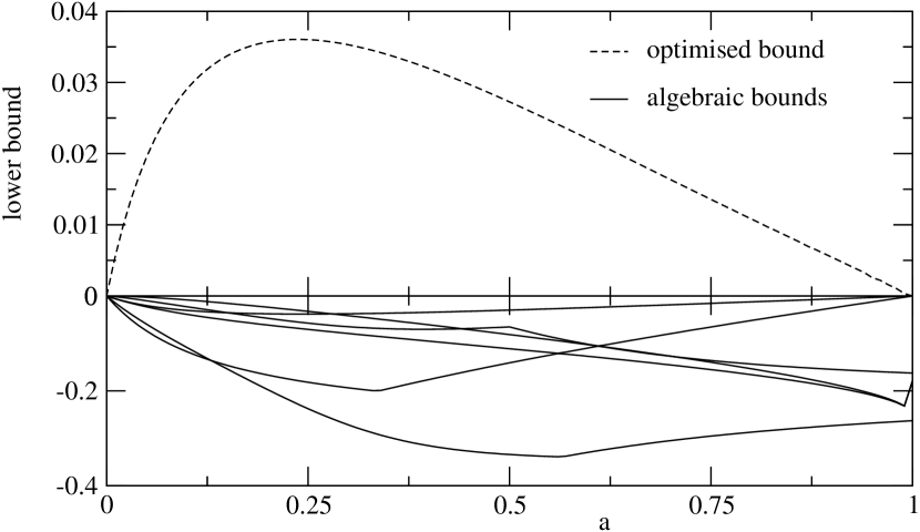
Figure 5: Algebraic lower bounds of the concurrence (see Eqs. (93) and (95), solid lines) of a family of $4\times 2$ states [75] defined by Eq. (103), plotted as a function of the parameter $a$. Although none of these bounds is positive, the optimised bound (dashed line), Eq. (93), is positive. Thus the state is detected as entangled in the entire parameter range of $a$.

A second class of states $\varrho_{a}$ [75] acts on ${\mathbbm{C}}^{4}\otimes{\mathbbm{C}}^{2}$, and once again has a positive partial transpose, Eq. (12), for $a\in[0,1]$:

$$\varrho_{a}=\frac{1}{1+7a}\left[{\begin{array}[]{ccccccccc}a&0&0&0&0&a&0&0\\ 0&a&0&0&0&0&a&0\\ 0&0&a&0&0&0&0&a\\ 0&0&0&a&0&0&0&0\\ 0&0&0&0&\beta&0&0&\gamma\\ a&0&0&0&0&a&0&0\\ 0&a&0&0&0&0&a&0\\ 0&0&a&0&\gamma&0&0&\beta\end{array}}\right],\hskip 14.22636pt\mbox{with}\hskip 14.22636pt\left\{\begin{array}[]{l}\displaystyle\beta=\frac{1+a}{2}\ ,\\ \left.\right.\\ \displaystyle\gamma=\frac{\sqrt{1-a^{2}}}{2}\ .\end{array}\right.$$ (103)

Figure 5 shows the algebraic lower bounds obtained as discussed in Section 3.1, which are all negative. Thus, none of them detects $\varrho_{a}$ as entangled. Though, due to the degeneracy of this particular state, there is a degeneracy in the eigenvalues of ${\cal A}$, such that the matrices $T^{\alpha}$, and, consequently, also the algebraic lower bounds, are not uniquely determined. Neither did we find any matrices $T^{\alpha}$ in the degenerate subspaces that provide positive lower bounds. Yet, the numerically optimised lower bound - also shown in Fig. 5 - is positive in the entire parameter range. Hence, also this state is detected as entangled by our lower bound, Eq. (93).

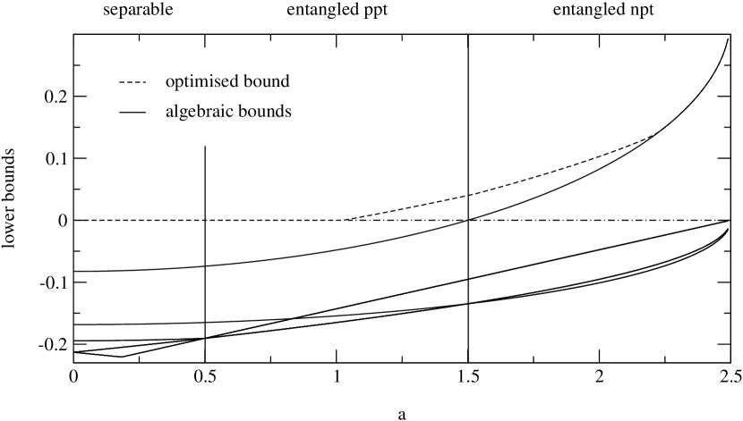
Figure 6: Algebraic lower bounds (see Eqs. (93) and (95), solid lines) of a family of $3\times 3$ states  [40] defined in Eq. (104), as a function of the parameter $a$. For $a\leq 1/2$, $\varrho_{a}$ is separable, and for $a>1/2$ it is entangled [40]. It has positive partial transpose for $a\leq 3/2$, and non-positive partial transpose for $a>3/2$. The dashed line shows the numerically optimised lower bound, Eq. (93). The state $\varrho_{a}$ is detected as entangled by the algebraic bound, exactly in that parameter range where it has non-positive partial transpose. It is detected as entangled by the optimised bound in approximately half the parameter range with positive partial transpose, what, however, might be due to a failure of our numerical optimisation routine.

A third class of states $\varrho_{a}$ [40], acting on ${\mathbbm{C}}^{3}\otimes{\mathbbm{C}}^{3}$, is defined for $a\in[-5/2,5/2]$,

$$\varrho_{a}=\frac{1}{21}\left[{\begin{array}[]{ccccccccc}2&0&0&0&2&0&0&0&2\\ 0&\beta_{-}&0&0&0&0&0&0&0\\ 0&0&\beta_{+}&0&0&0&0&0&0\\ 0&0&0&\beta_{+}&0&0&0&0&0\\ 2&0&0&0&2&0&0&0&2\\ 0&0&0&0&0&\beta_{-}&0&0&0\\ 0&0&0&0&0&0&\beta_{-}&0&0\\ 0&0&0&0&0&0&0&\beta_{+}&0\\ 2&0&0&0&2&0&0&0&2\end{array}}\right],\hskip 14.22636pt\mbox{with}\hskip 14.22636pt\beta_{\pm}=\frac{5}{2}\pm a\ .$$ (104)

Since replacing $a$ by $-a$ is equivalent to exchanging the subsystems, we will discuss this state only for $a\in[0,5/2]$. The state $\varrho_{a}$ has a non-positive partial transpose for $a\in[3/2,5/2]$, is entangled with positive partial transpose for $a\in[1/2,3/2]$ and is separable for $a\in[0,1/2]$ [40]. As depicted in Fig. 6, $\varrho_{a}$ is detected as entangled in its domain of negative partial transpose already by the best algebraic lower bound. In the regime where $\varrho_{a}$ has positive partial transpose all algebraic bounds are negative, such that the optimised lower bound is required for distinguishing $\varrho_{a}$ from separable states. However, even the optimised bound does not detect $\varrho_{a}$ in the entire interval $a\in[1/2,3/2]$. For $a\lesssim 1.02$, the lower bound seems to fail as a sufficient separability criterion. At present, we have no conclusive evidence from our numerical optimisationroutine to decide whether the bound itself is not good enough, or whether the numerically found maximum is not the global one.

The above exemplary $ppt$ states show that our lower bound, Eq. (93), is capable to detect families of entangled states which are not recognised by the $ppt$ criterion. For some states it is even not necessary to evaluate the optimised bound, since already one of the algebraic bounds, introduced in Section 3.1, is positive. Moreover, also the quasi-pure approximation is positive for some $ppt$ states [31]. However, there are also states with only negative algebraic bounds and negative quasi-pure approximation, though positive optimised bound. Our last example above showed a case of entangled states that we have so far been unable to detect for a small subset of parameters, though it remains hitherto undecided whether this is a failure of our numerical optimisation routine or of our lower bound, Eq. (93), itself. It is obvious from the different behaviour of optimised and algebraic bounds at the border line between ppt and non-ppt regions in Fig. 6, that some more profound algebraic signatures remain to be uncovered.

4 Dynamics of entanglement under environment coupling

Arguably the central motivation for deriving efficiently evaluable measures of the entanglement of mixed states is the ubiquity of the latter in any real physical setting. If we consider entanglement as the central resource of most types of quantum information processing, then the experimentally most relevant question is that of the lifetime of entanglement under the environment-induced mixing. This is the subject of the present, concluding section of this review.

In a first subsection, we will test the mixed state entanglement estimates derived in the previous sections, such as to demonstrate their versatility to describe generic time evolutions under environment coupling. Here, the time evolution both of the system and of the bath will be generated by random Hamiltonians, without any specific physical realization in mind.

Subsequently, we will specialise to particular, experimentally relevant (since realized) cases, and specifically focus on the scaling properties of the typical time scales which determine the time evolution of bipartite and multipartite entanglement.

4.1 Random time evolution of higher-dimensional bipartite systems

Let us first have a closer look at the performance of the various entanglement estimates derived above, for a generic time evolution under environment coupling. For that purpose, we consider a bipartite system and a third system serving as environment. The bipartite system is initially prepared in a maximally entangled pure state

$$|\varPhi_{0}\rangle=\frac{1}{\sqrt{d}}\sum_{i=1}^{d}|ii\rangle\ ,$$ (105)

i.e. , it is not entangled with the environment. We then evolve the total system under a unitary dynamics generated by the Hamiltonian

$$H=H_{\rm se}+H_{\rm s}\otimes{\mathbbm{1}}_{\rm e}+{\mathbbm{1}}_{\rm s}\otimes H_{\rm e},$$ (106)

with a randomly chosen hermitian matrix $H_{\rm se}$ acting on system and environment, while a second randomly chosen hermitian matrix $H_{\rm s}$ only acts on the (bipartite) system, but not on the environment. All elements of $H_{\rm se}$ and $H_{\rm s}$ are determined independently under the constraint of hermiticity. Any real entry is obtained as $\sin(r)$, with a random integer $r$, where the a priori probability is the same for any integer $0\leq r<10^{15}$ [77]. Furthermore, we neglect the free evolution of the environment by setting $H_{\rm e}={\mathbbm{1}}_{\rm e}$.

Tracing out the environment after a finte interaction time $t$ leads to a mixed state of the bipartite system. $H_{\rm s}$ describes the interaction between the bipartite system’s components and does not induce any mixing, though it can change the degree of entanglement. We further scale the Hamiltonians $H_{\rm se}$ and $H_{\rm s}$ by the real coupling constants $\alpha_{\rm se}$ and $\alpha_{\rm s}$, which fix the relative time scales of unitary and incoherent system dynamics. $\alpha_{\rm se}$ determines the strength of the system-environment interaction, and therefore the mixing rate of the system, whereas $\alpha_{\rm s}$ specifies the time-scale of the unitary system evolution, causing a reversible decrease and increase of bipartite entanglement therein.

Figure 7: Top panel: Upper bound (Eq. (79), solid line) and numerically optimised lower bound (Eqs. (93) and (94), dashed line) of concurrence of a $3\times 3$ state, vs. scaled time $\alpha_{\rm s}t$. The system is initially prepared in a maximally entangled state of type (105), with concurrence $c=2/\sqrt{3}$ (see Eq. (61)). A random time evolution according to (106), with $\alpha_{\rm se}/\alpha_{\rm s}=10^{-2}$, leads to a finite degree of mixing measured by the system state’s von Neumann entropy (dash-dotted line). The largest eigenvalue of $\varrho$ evolves along the dash-double-dotted line. In the lower panel, the solid and the dashed line represent the difference between the optimized lower bound of concurrence, Eqs. (93) and (94), and the quasi-pure approximation, Eq. (99), or the best algebraic lower bound, Eqs. (93) and (95), respectively. As also visible from the upper panel, all our lower bounds provide excellent estimates of the actual value of concurrence over the entire evolution period, almost undistinguishable from the upper bound, Eq. (79) (full line in the upper panel).

With these premises, we can now monitor the time evolution of the concurrence under the above random dynamics, as a function of the scaled time $\alpha_{\rm s}t$, for different values of the ratio $\alpha_{\rm se}/\alpha_{\rm s}$. The degree of mixing of $\varrho$ will be characterised by the von Neumann entropy $S=-\mbox{Tr}\varrho\ln\varrho$ of the system state. In addition, we also follow the time evolution of the largest eigenvalue of $\varrho$, since this was the central pillar in our derivation of the quasi-pure approximation (Section 3.2).

Figure 8: Same as Fig. 7, with a larger environment coupling constant $\alpha_{\rm se}/\alpha_{\rm s}=5\times 10^{-2}$.

The upper panels in Figs. 7 and 8 show the time evolution of upper (Eq. (79), solid line) and lower (Eqs. (93) and (94), dashed line) bounds of concurrence, together with concurrence in quasi-pure approximation (Eq. (99), dotted line), for two different random time evolutions of the same maximally entangled $3\times 3$ initial state. The initial value of $c(\varrho)$ follows immediately from Eq. (61). The interaction Hamiltonians $H_{\rm se}$ and $H_{\rm s}$ are the same in both figures, but the coupling constant $\alpha_{\rm se}$ in Fig. 8 is by a factor five larger as compared to its value $\alpha_{\rm se}/\alpha_{\rm s}=10^{-2}$ in Fig. 7. Consequently, mixing increases slower in Fig. 7 than in Fig. 8. The degree of mixing is characterised by both the largest eigenvalue of $\varrho$, depicted as a dash-double-dotted line, and by its von Neumann entropy (dash-dotted).

Figure 9: Same as Fig. 7, for a $4\times 4$ system initially prepared in the maximally entangled state, Eq. (105), and $\alpha_{\rm se}/\alpha_{\rm s}=10^{-2}$.

For both values of $\alpha_{\rm se}/\alpha_{\rm s}$, the quasi-pure approximation and the optimized lower bound remain almost indistinguishable, over the entire system-environment interaction time. The difference of both quantities is plotted in the lower panels of the figures, together with the difference between the numerically optimised lower bound, Eqs. (93) and (94), and the best algebraic bound, Eqs. (93) and (95). Over almost the entire time interval displayed in Fig. 7, and for short times in Fig. 8, where mixing is not too large, the relative error of both approximations is about two orders of magnitude smaller than the actual value of concurrence itself (note the different scales on the vertical axes). Only states with rather small concurrence and a large degree of mixing exhibit a significant difference between the optimized lower bound and the best algebraic bound or the quasi-pure approximation.

Figure 10: Same as in Figs. 7 and 9, for a $2\times 4$ system initially prepared in the maximally entangled state, Eq. (105), and $\alpha_{\rm se}/\alpha_{\rm s}=10^{-2}$.

Fig. 9 repeats the scenario of Fig. 7, for a $4\times 4$ system, with environment coupling constant $\alpha_{\rm se}/\alpha_{\rm s}=10^{-2}$. The degree of mixing remains moderate during the entire time evolution, as indicated by the von Neumann entropy and the largest eigenvalue of $\varrho$. Once again, in this higher-dimensional system, upper, Eq. (79), and optimised lower bound, Eq. (93) and (94), provide an excellent estimation of the actual value of concurrence. Equally so, also the best algebraic lower bound, Eqs. (93) and (95), and the quasi-pure approximation perform very well, over the entire time interval.

Figure 11: Same as Fig. 10, but for a larger system-environment coupling $\alpha_{\rm se}/\alpha_{\rm s}=5\times 10^{-2}$.

Qualitatively the same observations are made for the time evolution of an initially maximally entangled state, Eq. (105), of a $2\times 4$ system, monitored in Figs. 10 and 11, for different system-environment coupling strengths $\alpha_{\rm se}/\alpha_{\rm s}=10^{-2}$ and $5\times 10^{-2}$, respectively. Only during a rather short time interval, when concurrence exhibits a dip at $\alpha_{\rm s}t\simeq 3\times 10^{-4}$ in Fig. 11 does the discrepancy between optimal lower bound and its estimates increase to about one percent of the actual value of concurrence, which, however, rather highlights the excellent reliability of our estimates for all practical purposes. In particular, this holds true for the quasi-pure approximation, albeit the strongly mixed states occuring as time evolves in Fig. 11 hardly satisfy the basic assumptions made for its derivation (see Section 3.2).

4.2 Realistic scenarios of entanglement dynamics

Recently, many groups were able to prepare entangled states in a variety of physical systems and experimental setups, demonstrating an impressive ability to manipulate and detect them efficiently [7, 8, 9, 10, 11, 12, 13, 14, 15, 16, 17]. Particular effort has been devoted to entangle multiple subsystems, not only to investigate the possibility of fulfilling the fundamentally important scalability requirements for quantum computation, but also to understand how far one can push a quantum system towards the macroscopic limit and still observe entanglement - an intrinsic quantum feature with no classical counterpart.

However, a major obstacle for the controlled entanglement of more and more subsystems remains with the incapacity of achieving perfect screening of the system from the environment. After some time, the unavoidable residual interaction with the reservoir induces mixing of the system state, and thus the emergence of classical correlations, at the expense of quantum entanglement. Hence, we face the highly relevant task of understanding the sources of entanglement decay, what implies the identification of the associated time scales.

Although a general solution to this problem, for arbitrary system dynamics and decoherence mechanisms is still out of reach, our technical machinery developed in the previous sections allows to treat arguably all situations encountered in typical state of the art experiments, as we shall outline in the sequel. We start with a short recollection of environment models adapted for decoherence processes in a typical quantum optical context.

4.2.1 Environment models

We already anticipated in Section 4.1 that an open system can be described as a system $S$ which interacts with an environment $E$, such that the dynamics of the total system $S+E$ is unitary, and governed by the von-Neumann equation

$$\frac{d{\varrho}_{se}}{dt}=-\frac{i}{\hbar}\left[H,{\varrho}_{se}\right],$$ (107)

with the total Hamiltonian of the form (106). However, we are only interested in the properties of the system $S$ itself. An equation for the evolution of the (reduced) system density matrix $\varrho$ is obtained by performing a trace over the environmental degrees of freedom:

$$\frac{d{\varrho}}{dt}=-\frac{i}{\hbar}\mbox{Tr}_{e}\left[H,{\varrho}_{se}\right]\ .$$ (108)

In Section 4.1 we considered $S$ as a bipartite system and explicitely performed the total evolution given by $H$, obtaining the reduced density matrix after tracing over environmental degrees of freedom. However, an equation only for the density matrix of the system, after an interaction time $t$, can be obtained. Under the assumption of complete positivity and Markovian dynamics, it can be written in the Lindblad form [78, 79, 80]

$$\frac{d{\varrho}}{dt}=-\frac{i}{\hbar}\left[H_{S},\varrho\right]+{\cal L}\varrho=-\frac{i}{\hbar}\left[H_{S},\varrho\right]+\sum_{i}\frac{\Gamma_{i}}{2}\left(2\,{d}_{i}\,{\varrho}\,{d}_{i}^{\dagger}-{d}_{i}^{\dagger}\,{d}_{i}\,{\varrho}-{\varrho}\,{d}_{i}^{\dagger}\,{d}_{i}\right)\,,$$ (109)

where operators ${d}_{i}$ describe the system-environment coupling, with strength $\Gamma_{i}$. The use of the Markovian approximation is well justified in a large variety of quantum optical experiments where entanglement has been produced, although one should mention that non-Markovian effects can be important in the description of some condensed-matter systems [81].

Different situations may arise when a system is coupled to the environment: energy can be exchanged and dissipation can take place, noise can be added to the system, or elastic processes can introduce loss of phase coherence without energy transfer. All these processes can be described in terms of the above master equation by a suitable choice of the operators ${d}_{i}$, which can be written, in the case of two-level systems, in terms of the Pauli matrices. For a two-level system interacting with a thermal bath, for example, the non-unitary part of the master equation reads [82]

$${\cal L}\varrho=\frac{\Gamma(\bar{n}+1)}{2}\left(2\,\sigma_{-}\varrho\sigma_{+}-\sigma_{+}\sigma_{-}\varrho-\varrho\sigma_{+}\sigma_{-}\right)+\frac{\Gamma\bar{n}}{2}\left(2\,\sigma_{+}\varrho\sigma_{-}-\sigma_{-}\sigma_{+}\varrho-\varrho\sigma_{-}\sigma_{+}\right)\,.$$ (110)

In this equation, the first and the second term on the right hand side describe, respectively, decay and excitation processes, with rates which depend on the temperature, here parametrised by $\bar{n}$, the average thermal excitation of the reservoir. In the limit of vanishing temperature, ${\bar{n}}=0$, only the spontaneous decay term survives, leading to a purely dissipative process,

$$\frac{d{\varrho}}{dt}=\frac{\Gamma}{2}\left(2\,\sigma_{-}\varrho\sigma_{+}-\sigma_{+}\sigma_{-}\varrho-\varrho\sigma_{+}\sigma_{-}\right)\,,$$ (111)

which drives the system, asymptotically, to its ground state.

Another important limiting case of equation (110), which describes noisy dynamics, is obtained for infinite temperature, where $\bar{n}\rightarrow\infty$, and, simultaneously, $\Gamma\rightarrow 0$, so that $\Gamma\bar{n}\equiv\tilde{\Gamma}$ remains constant:

$${\cal L}\varrho=\frac{\tilde{\Gamma}}{2}\left(2\,\sigma_{-}\varrho\sigma_{+}-\sigma_{+}\sigma_{-}\varrho-\varrho\sigma_{+}\sigma_{-}\right)+\frac{\tilde{\Gamma}}{2}\left(2\,\sigma_{+}\varrho\sigma_{-}-\sigma_{-}\sigma_{+}\varrho-\varrho\sigma_{-}\sigma_{+}\right)\,.$$ (112)

In this case, decay and excitation occur at exactly the same rate, and the noise induced by the transitions between the two levels brings the system to a stationary, maximally mixed state.

A purely dephasing reservoir is obtained by choosing $d_{i}=d=\sigma_{+}\sigma_{-}$ in Eq. (109) leading to the master equation

$$\frac{d{\varrho}}{dt}=\frac{\Gamma}{2}\left(2\,\sigma_{+}\sigma_{-}\varrho\sigma_{+}\sigma_{-}-\sigma_{+}\sigma_{-}\varrho-\varrho\sigma_{+}\sigma_{-}\right)\,.$$ (113)

In this case, there are no changes in the populations of the ground and excited states, and energy is conserved. Only the off-diagonal elements of the reduced density matrix decay, leading to a loss of phase coherence.

In the context of entanglement, we have to describe how the environment acts on the composite system. In Sections 4.2.2 and 4.2.3 we will assume that each subsystem interacts independently with the environment, a well justified assumption whenever the particles composing your system are sufficiently separated from each other and, therefore, no collective environment effects must be taken into account. Hence, each particle is subjected to a dynamics described by its own Lindblad operator, supposed to be of the same form for all the components of the system. Note that this assumption of mutually independent environment couplings immediately implies that all initially entangled states will asymptotically evolve into a separable state. We shall therefore focus on the precise timescales of this decay process.

In the final Section 4.2.4, we will consider an entanglement scheme [83] which has been experimentally implemented using ion traps [9], and in which decoherence acts indirectly through the coupling of the collective center-of-mass motion of the ions with the environment. Here, again, environment interaction has a detrimental effect, which we shall study in more detail focusing on the scaling of multipartite entanglement with the system size (i.e., the number of entangled particles).

4.2.2 Entanglement dynamics of bipartite two-level systems

For bipartite two level systems, one can use the exact expression, Eq. (39), for concurrence, to follow the time evolution of entanglement. While much simpler than the multipartite case, the bipartite situation is useful for developing some intuition about the entanglement decay under different environment dynamics.

To start with, we consider an initial Bell state $|\Psi^{\pm}\rangle=\left(|01\rangle\pm|10\rangle\right)/\sqrt{2}$. The solution of the master equation for the different environment couplings discussed previously is straightforward, and the time evolution of concurrence, shown in Fig. 12, is given by

$$c(t)={\rm max}\left\{\frac{e^{-4\tilde{\Gamma}t}}{2}+e^{-2\tilde{\Gamma}t}-\frac{1}{2},0\right\}\,,$$ (114)

for the infinite temperature case, and by

$$c(t)=e^{-\Gamma t},$$ (115)

for dephasing, Eq. (113), and zero temperature, Eq. (111), environments. The situation is the same for the Bell state $|\Phi^{\pm}\rangle=\left(|00\rangle\pm|11\rangle\right)/\sqrt{2}$ (right panel of Fig. 12), apart from the zero temperature case where the concurrence decays as $c(t)=e^{-2\Gamma t}$. This accelerated (by a factor of two) decay of concurrence for the $|\Phi^{\pm}\rangle$ states as compared to the $|\Psi^{\pm}\rangle$ states, under the influence of zero temperature environment, can be understood from the time scales involved in the corresponding solution for the density matrix: while for $|\Phi^{\pm}\rangle$ each term $|01\rangle$ and $|10\rangle$ corresponds to a single particle decay, leading to a time scale $e^{-\Gamma t}$, we have the term $|11\rangle$ in $|\Psi^{\pm}\rangle$, such that both particles can undergo an environment induced transition to the ground state, thus introducing a faster, $e^{-2\Gamma t}$, decay. General solutions for the finite temperature case can be given explicitely [84], though are rather cumbersome and will not be presented here. However, one may expand these solutions and obtains, at first order in $t$,

$$c(\Psi^{\pm},t)\simeq 1-\left(2\bar{n}+1+2\sqrt{\bar{n}(\bar{n}+1)}\right)\Gamma t,$$ (116)

and

$$c(\Phi^{\pm},t)\simeq 1-2(2\bar{n}+1)\Gamma t,$$ (117)

for $|\Psi^{\pm}\rangle$ and $|\Phi^{\pm}\rangle$ states, respectively. These expressions not only reproduce the leading order terms of the zero and infinite temperature solutions in the appropriate limits, but also show the influence of the temperature on the short time behaviour of concurrence decay.

It is equally simple to obtain the long-time asymptotics for the singular values of the matrix $\tau$ defined in Section 2, and, consequently, for the quantity that enters expression (39) for concurrence. It reads, both for $|\Psi^{\pm}\rangle$ and $|\Phi^{\pm}\rangle$ states,

$$\lim_{t\to\infty}\left({\cal S}_{1}-\sum_{i=2}^{4}\ {\cal S}_{i}\right)=-\frac{2\bar{n}(\bar{n}+1)}{(2\bar{n}+1)^{2}}\ .$$ (118)

This quantity is non-positive for all values of $\bar{n}$ and vanishes only in the case of zero temperature. This means that the above initial states evolve into separable states within a finite time, for any $T>0$. In contrast, for zero temperature as well as for dephasing environments does $c(t)$ only vanish in the limit $t\rightarrow\infty$.

Figure 12: Time dependence of the concurrence of a bipartite two-level system initially prepared in Bell states $|\Psi^{\pm}\rangle$ (left panel) or $|\Phi^{\pm}\rangle$ (right panel), under coupling to a zero temperature (dotted lines), dephasing (long dashed lines), infinite (solid lines), and finite temperature ($\bar{n}=0.1$, dashed lines) environment (time evolution generated by Eqs. (111), (113), (112), and (110), respectively. In the case of $|\Psi^{\pm}\rangle$ states, the zero temperature and dephasing solutions coincide. In contrast, the zero temperature environment induces a twice as fast decay as compared to the dephasing environment, for the $|\Phi^{\pm}\rangle$ state. For all positive temperatures these initial states evolve into separable states in a finite time. Only zero temperature and dephasing environments induce separability only in the limit $t\rightarrow\infty$.

4.2.3 Entanglement dynamics of multipartite two-level systems

Let us now generalise our above investigation for larger arrays of two-level systems, with variable size $N$. These are objects often encountered, e.g., in ion trap quantum computing schemes, and the robustness of their entanglement properties with increasing size is at the very heart of the fundamental scalability requirement on which hinges any future technological application.

We have already prepared a comfortable tool for such generalisation – the multipartite concurrence $c_{N}$ defined in Eq. (88), with the particularly useful property

$$c_{N}(|\varPhi\rangle\otimes|\varphi\rangle) = c_{N-1}(|\varPhi\rangle)\ ,$$ (119)

$${\rm for}\ |\varPhi\rangle\otimes|\varphi\rangle \in {\cal H_{1}}\otimes\ldots\otimes{\cal H_{N}},\ {\rm and}\ |\varphi\rangle\in{\cal H_{i}},\ i\in\left\{1,\ldots,N\right\}\ .$$ (120)

This allows for the direct comparison of the entanglement properties of pure and mixed states of multipartite qubit arrays of increasing size [32], where the mixed state concurrence is once again evaluated through the convex roof Eq. (67), with the appropriate definition of the operator $A$ in Eq. (87).

Since the reliability of the lower bounds derived in Section 3 was demonstrated extensively in Section 4.1 above, we will actually use the quasi-pure approximation Eq. (99) in the following, minimising the numerical effort very considerably, notably for large system sizes $N$ (notwithstanding, some additional tests were performed at randomly chosen instances, to convince ourselves of the quality of the quasi-pure approximation with respect to the optimal upper and lower bounds, Eqs. (79) and (93), respectively.

We shall consider two types of initial states, somewhat similar to the singlet and triplet states in Section 4.2.2 above: the GHZ state

$$|\Psi_{N}\rangle_{\rm GHZ}=\frac{1}{\sqrt{2}}\left(|00\ldots 0\rangle+|11\ldots 1\rangle\right)\ ,$$ (121)

and the W state,

$$|\Psi_{N}\rangle_{W}=\frac{1}{\sqrt{N}}\left(|00\ldots 01\rangle+|00\ldots 10\rangle+\ldots+|10\ldots 00\rangle\right).$$ (122)

These were recently produced [9, 12] in the lab, for $N=3,4$, and it is now within experimental reach to monitor the time dependence of their degree of entanglement, by means of quantum state tomography [17]. Figure 13 shows the decay of the concurrence for tri-partite GHZ and W states under the influence of zero temperature (circles), dephasing (triangles) and infinite temperature (squares) environments as a function of time. The symbols represent the result of the quasi-pure approximation, while the lines indicate the best fit to a mono-exponential decay $c_{N}(t)=Ae^{-\gamma t}+B$. As in the bipartite case, the zero temperature and dephasing environment lead to separability only in the limit $t\to\infty$, for these initial states. 

Figure 13: Time dependence of the multipartite concurrence $c_{N}(t)$, Eq. (88), for $N=3$ particle systems initially prepared in a GHZ (dashed lines) or W (solid lines) state, under the influence of a zero temperature (circles), dephasing (triangles), and infinite temperature (squares) environments. In all cases, the numerical results are very well fitted by an exponential decay (solid and dashed lines).

To assess the scaling properties of multipartite entanglement for variable system size, we now compute the time evolution of concurrence, precisely as in Fig. 13, for different values of $N$, and extract the decay rates $\gamma$. Fig. 14 shows the scaling of the entanglement decay rates $\gamma$ with $N$, under the above, distinct decoherence mechanisms.

We see that the decay rate of the concurrence of GHZ states (top panel of the figure) increases linearly with $N$, except for the small-$N$ behaviour of $\gamma$ for the zero temperature environment. Indeed, in the special case of dephasing environment, the density matrix is always a mixture of two pure states, and, hence, of rank two, and can be treated analytically. The observed behaviour comforts our intuition – which suggests that the larger the system, the easier it is for detrimental environment effects to manifest. In addition, this fragility of GHZ states was also observed in [86] by an analysis based on their separability and distillability properties [87, 88] rather than a dynamical approach.

Remarkably, the situation changes quite drastically for the W states (bottom plot of Fig. 14). In this case, only the infinite temperature environment gives rise to an almost linear increase of $\gamma$ with $N$, slightly faster than for the GHZ states. In contrast, for dephasing and zero temperature reservoirs, the decay of the concurrence is independent of $N$. Moreover, the zero temperature case also allows for an analytic solution (as above, the rank of the state reduces to two) for all $N$, leading to $c_{N}(t)\sim e^{-\Gamma t}$. Consequently, for these environments, W states clearly outperform GHZ states in terms of the robustness of their multipartite entanglement properties.

One might be tempted to attribute this to the smaller initial concurrence of W as compared to GHZ states (see Fig. 13), though the ratio

$$\frac{c_{N}(\Psi_{GHZ})}{c_{N}(\Psi_{W})}=\sqrt{(1-2^{1-N})\frac{N}{N-1}}$$

with a maximum at $N=5$, approaches unity for large $N$ (with a value $1.07$ for $N=7$, the maximal size considered in Fig. 14).

Figure 14: Concurrence decay rates $\gamma$ (in units of the reservoir rate $\Gamma$) for GHZ (top) and W (bottom) states, as a function of the system size (i.e., the particle number) $N$. The different environment models are represented by circles (zero temperature), squares (infinite temperature), and triangles (dephasing). The connecting lines are drawn to guide the eye. Whilst for GHZ states the decay rates increase roughly linearly with $N$ (for sufficiently large $N$), independently of the specific environment, the W states exhibit increasing decay with system size only for the infinite temperature environment. Remarkably, the decay rate of the W states is size-independent for dephasing and zero temperature environments!

4.2.4 Experimental entanglement production: the Mølmer-Sørensen scheme

In the previous sections we assumed that a perfect pure entangled state is available at the beginning, and monitored the reservoir induced entanglement decay in the course of time. Here, we will consider a situation where the environment acts simultaneously to a unitary evolution which is intended to prepare the entangled state. Specifically, we scrutinize a scalable scheme proposed in [83] to produce GHZ-like states (see Eq. (121)),

$$|\Psi_{N}\rangle=\frac{1}{\sqrt{2}}\left(|00\ldots 0\rangle+e^{i\phi_{N}}|11\ldots 1\rangle\right)\ ,$$ (123)

experimentally implemented at NIST [9] to produce controlled entanglement of two and four trapped ions.

To illustrate this preparation scheme – which is valid for $N$ ions – let us consider the case $N=2$ with two ions confined by a harmonic potential, simultaneously illuminated by two electromagnetic fields. The energy levels are depicted in Fig. (15), where $\omega_{0}$ is the frequency of the electronic transition, and $\nu$ the oscillation frequency of a given collective motional mode of the particles in the trap. The fields oscillate with $\omega_{0}+\nu-\Delta$ and $\omega_{0}-\nu+\Delta$ in such a way that the two photon process that drives the $|00\rangle\leftrightarrow|11\rangle$ transition is resonant and a superposition of these states can be produced. At the end of the preparation scheme, all one-photon processes, which excite motional states, interfere destructively with each other, such that vibrational and internal degrees of freedom are uncorrelated. However, during the illumination these correlations do exist, and motional decoherence can decrease the success probability of the preparation process. The decay rate of the electronic states is negligible during the time scale of the state preparation, and therefore one of the main sources of errors in the system arises indirectly through the coupling with these decohering motional modes.

Figure 15: Illustration of the Mølmer-Sørensen scheme [83] for the creation of a maximally entangled state $(|00\rangle+i|11\rangle)/\sqrt{2}$. Two ions are illuminated simultaneously by two electro-magnetic fields. One (dashed arrows) is red detuned with respect to the blue sideband, with detuning $\Delta$. The second pump field (dotted arrows) is blue detuned with respect to the red sideband. Both sideband transitions are not driven resonantly, however the two photon process $|00\rangle\leftrightarrow|11\rangle$ is resonant, since the absolute values of the detunings of both transitions coincide. Thus, starting with the initial state $|00\rangle$, one can create a coherent superposition of the states $|00\rangle$ and $|11\rangle$.

The heating of the ions, related to fluctuating fields in the trap electrodes, leads to a thermal motion with steadily increasing temperature and can be well described by the infinite temperature reservoir discussed previously, Eq. (112), with measured heating rates $\Gamma/\nu$ ranging from $10^{-4}$ to $10^{-3}$ [89, 90].

Figure 16 shows the time evolution of the multipartite concurrence $c_{N}$, Eq. (88), (evaluated through its quasi-pure approximation, Eq. (99)) under this scheme, for four ions and heating rates $\Gamma/\nu=0$ (bold solid line), $1\times 10^{-4}$ (solid line), $2\times 10^{-4}$ (dashed line), $3\times 10^{-4}$ (dot-dashed line) and $4\times 10^{-4}$ (dotted line). The system starts with all ions in the electronic ground states and, during the evolution, entanglement builds up until reaching its maximum value at $\nu t_{prep}=\pi/(\eta\Omega)\simeq 1100$ (with $\eta$ the Lamb-Dicke parameter, the ratio between the width of the vibrational ground state and the wavelength of the driving radiation, and $\Omega$ the single ion resonant Rabi frequency describing the strength of ion-field coupling). After this preparation time the lasers should be turned off and, for zero environment coupling, concurrence achieves its ideal value corresponding to the GHZ-like state, while it shows appreciable decrease even for small heating rates.

Figure 16: Quasi-pure calculation (see Section 3.2) of the time evolution of the multipartite concurrence for four ions. In the case of vanishing environment coupling (bold solid line), concurrence reaches its ideal value at the preparation time $\nu t_{\rm prep}=\pi/(\eta\Omega)\simeq 1100$, with $\eta=0.05$ and $\Omega=0.057$. As we increase the coupling strength $\Gamma/\nu$, the maximally achievable entanglement decreases, as shown for $\Gamma/\nu=1\times 10^{-4}$ (solid line), $2\times 10^{-4}$ (dashed line), $3\times 10^{-4}$ (dot-dashed line) and $4\times 10^{-4}$ (dotted line).

As in the case of the purely environment induced dynamics, we are interested in the scaling of the achieved degree of entanglement with the system size $N$. In the ideal case, the maximum value of the multipartite concurrence, Eq. (88), increases with $N$ as $c_{N}=2^{1-N/2}\sqrt{(2^{N}-2)/2}$, saturating at $\sqrt{2}$ for large $N$ as depicted by the bold solid line and circles in Fig. 17. With the addition of motional heating, this growth with $N$ is not monotonic anymore and we observe, for example, that from a certain value of the coupling strength the maximum concurrence for six ions gets smaller than the one for five. Hence, the detrimental effect of (indirect) motional decoherence for entanglement generation is enhanced with increasing system size. This is further illustrated in Fig. 18, where we plot the entanglement loss $\Delta_{c}=c_{N}^{\rm GHZ}-c_{N}^{\rm max}$, i.e., the difference between the ideal value and the actual optimal value achieved at a finite decoherence level. For all values of the ion heating rate, the entanglement loss increases with the system size.

Figure 17: Maximally achievable concurrence $c_{N}^{max}$, as a function of the number of ions, for reservoir coupling $\Gamma/\nu=0$ (circles), $1\times 10^{-4}$ (squares), $2\times 10^{-4}$ (diamonds), $3\times 10^{-4}$ (triangles) and $4\times 10^{-4}$ (stars). The bold line shows the exact growth of the multipartite concurrence as a function of $N$ for GHZ-like states, which saturates at $\sqrt{2}$. This growth is not monotonic anymore when motional decoherence is considered, indicating that environment effects become more and more detrimental for growing system size.

Figure 18: Difference $\Delta_{c}=c_{N}^{\rm GHZ}-c_{N}^{\rm max}$ between the ideal and the maximally achievable concurrence, as a function of the system size $N$. Squares, diamonds, triangles and stars represent reservoir coupling strengths $\Gamma/\nu=1\times 10^{-4}$, $2\times 10^{-4}$, $3\times 10^{-4}$ and $4\times 10^{-4}$, respectively. Consistently with Fig. 17, the entanglement loss during the preparation process increases with $N$.

5 Conclusion

In the present contribution, we have performed a program reaching from the formal definition to the time dependent monitoring of concurrence of arbitrary, finite dimensional, multipartite quantum states under incoherent environment coupling. The general applicability of the various lower bounds of concurrence which have been derived stems from the algebraic structure of a suitable reformulation of its original definition, with direct generalizations for higher dimensional and/or multipartite quantum states.

We have checked the reliability and tightness of our various approximate lower bounds of concurrence under very different physical scenarios, from rather untypical entangled states with positive partial transpose to experimental schemes of controlled environment production. Whilst these results generally suggest a rather excellent performance of the here derived, efficiently computable entanglement measures, also quite a few questions remain to be answered on the mathematical side: Which of our lower bounds of concurrence are actually able to detect all entangled states? Are there analytical error bounds for the various approximations? Are there classes of entangled states which cannot be detected by our lower bounds? Is there a suitable generalization of our characterisation of multipartite entanglement through projectors on antisymmetric subspaces such as to have a complete description of multipartite quantum correlations? And is there a generalisation for continuous variable systems?

And on the physical side: Given the now possible monitoring of the time evolution of entanglement under environment coupling, how are the entanglement decay rates encoded in the coherences of the original density matrix? How do these decay rates depend on i) the initial state and ii) the environment coupling operators and strengths? And, perhaps most importantly: Since the Hilbert size dimension increases exponentially with increasing systems size (i.e. increasing number of system components), quantum state tomography will become inoperational to quantify the state’s entanglement properties. Which experimental observables are then best suited to fulfill this task? Or, in other words, which are the robust dynamical observables which exhibit a clear experimental signature of the various types of multipartite entanglement?

Hence, despite the considerable progresses on which we have reported here, a panoply of challenging open questions awaits solution, what simply reflects the potential – on the fundamental level as well as on the level of applications (from decoherence control to quantum computation) – of entanglement theory, a field still in its infancy, at the emerging interface of mathematical physics and experiments.

6 Acknowledgement

We are indebted to Rainer Blatt, Rafał Demkowicz-Dobrzański, Klaus Dietz, Berge Englert, Daniel Estève, Hartmut Häffner, Peter Hänggi, Armin Uhlmann, Thomas Wellens, and Karol Życzkowski, for inspiring discussions, fruitful suggestions, critical comments and pertinent remarks. Financial support by VolkswagenStiftung (under the project “Entanglement measures and the influence of noise”) and Polish MNiI grant No 1P03B04226 is gratefully acknowledged. This work was supported by a fellowship within the Postdoc- Programme of the German Academic Exchange Service (DAAD).

References

- [1] R. P. Feynman, Simulating physics with computers, Int. J. Theor. Phys. 21 (1982) 467.
- [2] D. Deutsch, Quantum theory, the church-turing principle and the universal quantum computer, Proc. R. Soc. Lond. A 425 (1985) 73.
- [3] C. H. Bennett, G. Brassard, C. Crépeau, R. Jozsa, A. Peres, W. K. Wootters, Teleporting an unknown quantum state via dual classical and einstein-podolsky-rosen channels, Phys. Rev. Lett. 70 (1993) 1895.
- [4] C. H. Bennet, G. Brassard, Quantum cryptography: Public key distribution and coin tossing, Proceedings of IEEE International Conference on Computers, Systems and Signal Processing (1984) 175.
- [5] C. Monroe, D. M. Meekhof, B. E. King, W. M. Itano, D. J. Wineland, Demonstration of a fundamental quantum logic gate, Phys. Rev. Lett. 75 (1995) 4714.
- [6] Q. A. Turchette, C. S. Wood, B. E. King, C. J. Myatt, D. Leibfried, W. M. Itano, C. Monroe, D. J. Wineland, Deterministic entanglement of two trapped ions, Phys. Rev. Lett. 81 (1998) 3631.
- [7] J.-W. Pan, D. Bouwmeester, M. D. H. Weinfurter, A. Zeilinger, Experimental test of quantum nonlocality in three-photon greenberger-horne-zeilinger entanglement, Nature 403 (2000) 515.
- [8] O. Mandel, M. Greiner, A. Widera, T. Rom, T. W. Hänsch, I. Bloch, Controlled collisions for multi-particle entanglement of optically trapped atoms, Nature 425 (2003) 937.
- [9] C. A. Sackett, D. Kielpinski, B. E. King, C. Langer, V. Meyer, C. J. Myatt, M. Rowe, Q. A. Turchette, W. M. Itano, D. J. Wineland, C. Monroe, Experimental entanglement of four particles, Nature 404 (2000) 256.
- [10] J.-W. Pan, M. Daniell, S. Gasparoni, G. Weihs, A. Zeilinger, Experimental demonstration of four-photon entanglement and high-fidelity teleportation, Phys. Rev. Lett. 86 (2001) 4435.
- [11] M. Eibl, N. Kiesel, M. Bourennane, C. Kurtsiefer, H. Weinfurter, Experimental realization of a three-qubit entangled w state, Phys. Rev. Lett. 92 (2004) 077901.
- [12] C. F. Roos, M. Riebe, H. Häffner, W. Hänsel, J. B. elm, G. P. T. Lancaster, C. Becher, F. Schmidt-Kaler, R. Blatt, Control and measurement of three-qubit entangled states, Science 304 (2004) 1478.
- [13] A. Rauschenbeutel, G. Nogues, S. Osnaghi, P. Bertet, M. Brune, J.-M. Raimond, S. Haroche, Step-by-step engineered multiparticle entanglement, Science 288 (2000) 2024.
- [14] Z. Zhao, Y.-A. Chen, A.-N. Zhang, T. Yang, H. J. Briegel, J.-W. Pan, Experimental demonstration of five-photon entanglement and open-destination teleportation, Nature 430 (2004) 54.
- [15] Y. A. Pashkin, T. Yamamoto, O. Astafiev, Y. Nakamura, D. V. Averin, J. S. Tsai, Quantum oscillations in two coupled charge qubits, Nature 421 (2003) 823.
- [16] A. J. Berkley, H. Xu, R. C. Ramos, M. A. Gubrud, F. W. Strauch, P. R. Johnson, J. R. Anderson, A. J. Dragt, C. J. Lobb, F. C. Wellstood, Entangled macroscopic quantum states in two superconducting qubits, Science 300 (2003) 1548.
- [17] C. F. Roos, G. P. T. Lancaster, M. Riebe, H. Häffner, W. Hänsel, S. Gulde, C. Becher, J. Eschner, F. Schmidt-Kaler, R. Blatt, Bell states of atoms with ultralong lifetimes and their tomographic state analysis, Phys. Rev. Lett. 92 (2004) 220402.
- [18] J. S. Bell, On the einstein-podolski-rosen paradox, Physics 1 (1964) 195.
- [19] J. F. Clauser, M. A. Horne, A. Shimony, R. A. Holt, Proposed experiment to test local hidden-variable theories, Phys. Rev. Lett. 23 (1969) 880.
- [20] C. Papaliolios, Experimental test of a hidden-variable quantum theory, Phys. Rev. Lett. 18 (1967) 622.
- [21] A. Einstein, B. Podolsky, N. Rosen, Can quantum-mechanical description of physical reality be considered complete ?, Phys. Rev. 47 (1935) 777.
- [22] D. M. Greenberger, M. A. Horne, A. Shimony, A. Zeilinger, Bell’s theorem without inequalities, Am. J. Phys. 58 (1990) 1131.
- [23] C. H. Bennett, H. J. Bernstein, S. Popescu, B. Schumacher, Concentrating partial entanglement by local operations, Phys. Rev. A 53 (1996) 2046.
- [24] C. H. Bennett, D. P. DiVincenzo, J. A. Smolin, W. K. Wootters, Mixed-state entanglement and quantum error correction, Phys. Rev. A 54 (1996) 3824.
- [25] G. Vidal, Entanglement monotones, J. Mod. Opt 47 (2000) 355.
- [26] G. Vidal, R. F. Werner, Computable measure of entanglement, Phys. Rev. A 65 (2002) 032314.
- [27] W. K. Wootters, Entanglement of formation of an arbitrary state of two qubits, Phys. Rev. Lett. 80 (1998) 2245.
- [28] T. Wellens, M. Kuś, Separable approximation for mixed states of composite quantum systems, Phys. Rev. A 64 (2001) 052302.
- [29] B.-G. Englert, N. Metwally, Remarks on 2-q-bit states, Appl. Phys. B 72 (2001) 35.
- [30] F. Mintert, M. Kuś, A. Buchleitner, Concurrence of mixed bipartite quantum states in arbitrary dimensions, Phys. Rev. Lett. 92 (2004) 167902.
- [31] F. Mintert, A. Buchleitner, Concurrence of quasi pure quantum states, quant-ph/0411130.
- [32] A. R. R. Carvalho, F. Mintert, A. Buchleitner, Decoherence and multipartite entanglement, Phys. Rev. Lett. 93 (2004) 230501.
- [33] F. Schwabl, Quantenmechanik, Springer Verlag, Berlin, 1998.
- [34] R. F. Werner, Quantum states with einstein-podolsky-rosen correlations admitting a hidden-variable model, Phys. Rev. A 40 (1989) 4277.
- [35] P. A. Horn, C. R. Johnson, Matrix Analysis, Cambridge University Press, New York, 1985.
- [36] K. Kraus, States, Effects and Operations, Springer Verlag, Berlin, 1983.
- [37] M. Horodecki, P. Horodecki, R. Horodecki, Separability of mixed states: necessary and sufficient conditions, Phys. Lett. A 223 (1996) 1.
- [38] A. Peres, Separability criterion for density matrices, Phys. Rev. Lett. 77 (1996) 1413.
- [39] M. Horodecki, P. Horodecki, R. Horodecki, Mixed-state entanglement and distillation: Is there a ‘bound’ entanglement in nature?, Phys. Rev. Lett. 80 (1998) 5239.
- [40] P. Horodecki, M. Horodecki, R. Horodecki, Bound entanglement can be activated, Phys. Rev. Lett. 82 (1999) 1056.
- [41] C. H. Bennet, D. P. DiVincenzo, J. Smolin, W. K. Wootters, Mixed-state entanglement and quantum error correction, Phys. Rev. A 54 (1996) 3824.
- [42] K. Kraus, General state changes in quantum theory, Ann. Phys. 64 (1971) 311.
- [43] M. A. Nielsen, I. L. Chuang, Quantum computation and quantum information, Cambridge University Press, 2000.
- [44] K. E. Hellwig, K. Kraus, Pure operations and measurements, Commun. Math. Phys. 11 (1969) 214.
- [45] K. E. Hellwig, K. Kraus, Operations and measurements ii, Commun. Math. Phys. 16 (1970) 142.
- [46] C. H. Bennett, D. P. DiVincenzo, C. A. Fuchs, T. Mor, E. Rains, P. W. Shor, J. A. Smolin, W. K. Wootters, Quantum nonlocality without entanglement, Phys. Rev. A 59 (1999) 1070.
- [47] M. A. Nielsen, Conditions for a class of entanglement transformations, Phys. Rev. Lett. 83 (1999) 436.
- [48] T. Ando, Majorization, doubly stochastic matrices, and comparison of eigenvalues, Linear Algebra Appl. 118 (1989) 163.
- [49] A. Uhlmann, Fidelity and concurrence of conjugated states, Phys. Rev. A 62 (2000) 032307.
- [50] L. P. Hughston, R. Jozsa, W. K. Wootters, A complete classification of quantum ensembles having a given density matrix, Phys. Lett. A 183 (1993) 14.
- [51] E. Schrödinger, Probability relations between separated systems, Proc. Cambridge Philos. Soc 32 (1936) 446.
- [52] A. Uhlmann, Optimizing entropy relative to a channel or a subalgebra, Open Sys. & Inf. Dyn. 5 (1998) 209.
- [53] V. Vedral, M. Plenio, Entanglement measures and purification procedures, Phys. Rev. A 57 (1998) 1619.
- [54] D. Bruß, Characterizing entanglement, J. Math. Phys. 43 (2002) 4237.
- [55] M. Horodecki, Entanglement measures, Quant. Inf. Comp. 1 (2001) 3.
- [56] M. Horodecki, P. Horodecki, J. Oppenheim, Reversible transformations from pure to mixed states and the unique measure of information, Phys. Rev. A 67 (2003) 062104.
- [57] S. Hill, W. K. Wootters, Entanglement of a pair of quantum bits, Phys. Rev. Lett. 78 (1997) 5022.
- [58] E. W. Weisstein, Concise Encyclopedia of Mathematics, CRC press, London, 1999.
- [59] B. M. Terhal, K. G. H. Vollbrecht, Entanglement of formation for isotropic states, Phys. Rev. Lett 85 (2000) 2625.
- [60] G. Vidal, W. Dür, J. I. Cirac, Entanglement cost of bipartite mixed states, Phys. Rev. Lett. 89 (2002) 027901.
- [61] F. Benatti, H. Narnhofer, Additivity of the entanglement of formation, Phys. Rev. A 63 (2001) 042306.
- [62] A. A. Pomeransky, Strong superadditivity of the entanglement of formation follows from its additivity, Phys. Rev. A 68 (2003) 032317.
- [63] K. Życzkowski, Volume of the set of separable states. ii, Phys. Rev. A 60 (1999) 3496.
- [64] K. Audenaert, F. Verstraete, B. D. Moor, Variational characterizations of separability and entanglement of formation, Phys. Rev. A 64 (2001) 052304.
- [65] A. Łozinski, A. Buchleitner, K. Życzkowski, T. Wellens, Entanglement of quantum systems, Euro Phys. Lett. 62 (2003) 168.
- [66] W. K. Wootters, Entanglement of formation and concurrence, Quant. Inf. Comp. 1 (2001) 27.
- [67] P. Rungta, V. Buzek, C. M. Caves, M. Hillery, G. J. Milburn, Universal state inversion and concurrence in arbitrary dimensions, Phys. Rev. A 64 (2001) 042315.
-
[68]
F. Mintert, Measures and dynamics of quantum entanglement, Ph.D. thesis,
Ludwig-Maximilians-Universität München (2004).
URL http://edoc.ub.uni-muenchen.de/archive/00002133 - [69] G. H. Golub, C. F. VanLoan, Matrix Computations, Johns Hopkins Univ. Pr., 1996.
- [70] W. Dür, G. Vidal, J. I. Cirac, Three qubits can be entangled in two inequivalent ways, Phys. Rev. A 62 (2000) 062314.
- [71] V. Coffman, J. Kundu, W. K. Wootters, Distributed entanglement, Phys.Rev. A 61 (2000) 052306.
- [72] G. Rigolin, Quantum teleportation of an arbitrary two qubit state and its relation to multipartite entanglement, Phys. Rev. A 71 (2005) 032321.
- [73] E. Beckenbach, R. E. Bellmann, Inequalities, Springer Verlag, Berlin, 1971.
- [74] K. Eckert, J. Mompart, X. X. Yi, J. Schliemann, D. Bruß, G. Birkl, M. Lewenstein, Quantum computing in optical microtraps based on the motional states of neutral atoms, Phys. Rev. A 66 (2002) 042317.
- [75] P. Horodecki, Separability criterion and inseparable mixed states with positive partial transposition, Phys. Lett. A 232 (1997) 333.
- [76] W. H. Press, S. A. Teulosky, W. T. Vetterling, B. P. Flannery, Numerical Recipies, Cambridge University Press, Cambridge, 1999.
- [77] G. Krüger, Programmieren in C, Addison-Wesley, Bonn, 1996.
- [78] G. Lindblad, On the generators of quantum dynamical semigroups, Math. Phys. 48 (1976) 119.
- [79] V. Gorini, A. Kossakowski, E. C. G. Sudarshan, Completely positive dynamical semigroups of n-level systems, J. Math. Phys. 17 (1976) 821.
- [80] R. Alicki, K. Lendi, Quantum Dynamical Semigroups and Applications, Lecture Notes in Physics 286, Springer-Verlag, Berlin, 1987.
- [81] A. V. Khaetskii, D. Loss, L. Glazman, Electron spin decoherence in quantum dots due to interaction with nuclei, Phys. Rev. Lett. 88 (2002) 186802.
- [82] S. M. Barnett, P. Radmore, Methods in Theoretical Quantum Optics, Clarendon Press, Oxford, 1997.
- [83] K. Mølmer, A. Sørensen, Multiparticle entanglement of hot trapped ions, Phys. Rev. Lett. 82 (1999) 1835.
- [84] A. R. R. Carvalho, et al., in preparation.
- [85] T. Yu, J. H. Eberly, Finite-time disentanglement via spontaneous emission, Phys. Rev. Lett. 93 (2004) 140404.
- [86] W. Dür, H.-J. Briegel, Stability of macroscopic entanglement under decoherence, Phys. Rev. Lett. 92 (2004) 180403.
- [87] W. Dür, J. I. Cirac, R. Tarrach, Separability and distillability of multiparticle quantum systems, Phys. Rev. Lett. 83 (1999) 3562.
- [88] W. Dür, J. I. Cirac, Classification of multiqubit mixed states: separability and distillability properties, Phys. Rev. A 61 (2000) 042314.
- [89] Q. A. Turchette, D. Kielpinski, B. E. King, D. Leibfried, D. M. Meekhof, C. J. Myatt, M. A. Rowe, C. A. Sackett, W. M. Itano, C. Monroe, D. J. Wineland, Heating of trapped ions from the quantum ground state, Phys. Rev. A 61 (2000) 063418.
- [90] Q. A. Turchette, C. J. Myatt, B. E. King, C. A. Sackett, D. Kielpinski, W. M. Itano, C. Monroe, D. J. Wineland, Decoherence and decay of motional quantum states of a trapped atom coupled to engineered reservoirs, Phys. Rev. A 62 (2000) 053807.