Analysis of Popper’s Experiment and its Realization

Abstract

An experiment proposed by Karl Popper to test the standard interpretation of quantum mechanics was realized by Kim and Shih. We use a quantum mechanical calculation to analyze Popper’s proposal, and find a surprising result for the location of the virtual slit. We also analyze Kim and Shih’s experiment, and demonstrate that although it ingeniously overcomes the problem of temporal spreading of the wave-packet, it is inconclusive about Popper’s test. We point out that another experiment which (unknowingly) implements Popper’s test in a conclusive way, has actually been carried out. Its results are in contradiction with Popper’s prediction, and agree with our analysis.

1 Introduction

The evidently nonlocal character of quantum mechanics has been a source of discomfort right from the time of its inception. Einstein Podolsky and Rosen, in their seminal paper, introduced a thought experiment, which became famous as the EPR experiment, articulating the disagreement of quantum theory with the classical notion of locality [1].

A lesser known experiment was proposed by Karl Popper, who called it a variant of the EPR experiment, to test the standard interpretation of quantum theory [2, 3]. Popper’s proposed experiment consists of a source $S$ that can generate pairs of particles traveling to the left and to the right along the $x$-axis. The momentum along the $y$-direction of the two particles is entangled in such a way so as to conserve the initial momentum at the source, which is zero. There are two slits, one each in the paths of the two particles. Behind the slits are semicircular arrays of detectors which can detect the particles after they pass through the slits (see Fig. 1).

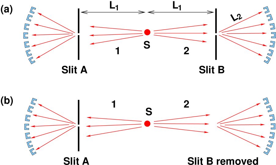
Figure 1: Schematic diagram of Popper’s thought experiment. (a) With both slits, the particles are expected to show scatter in momentum. (b) By removing slit B, Popper believed that the standard interpretation of quantum mechanics could be tested.

Being entangled in momentum space implies that in the absence of the two slits, if a particle on the left is measured to have a momentum $p$, the particle on the right will necessarily be found to have a momentum $-p$. One can imagine a state similar to the EPR state, $\psi(y_{1},y_{2})=\!\int_{-\infty}^{\infty}e^{ipy_{1}/\hbar}e^{-ipy_{2}/\hbar}dp$. As we can see, this state also implies that if a particle on the left is detected at a distance $y$ from the horizontal line, the particle on the right will necessarily be found at the same distance $y$ from the horizontal line. It appears, however, that a hidden assumption in Popper’s setup is that the initial spread in momentum of the two particles is not very large. Popper argued that because the slits localize the particles to a narrow region along the $y$-axis, they experience large uncertainties in the $y$-components of their momenta. This larger spread in the momentum will show up as particles being detected even at positions that lie outside the regions where particles would normally reach based on their initial momentum spread. This is generally understood as a diffraction spread.

Popper suggested that slit B be made very large (in effect, removed). In this situation, Popper argued that when particle 1 passes through slit A, it is localized to within the width of the slit. He further argued that the standard interpretation of quantum mechanics tells us that if particle 1 is localized in a small region of space, particle 2 should become similarly localized, because of entanglement. The standard interpretation says that if one has knowledge about the position of particle 2, that should be sufficient to cause a spread in the momentum, just from the Heisenberg uncertainty principle. Popper said that he was inclined to believe that there will be no spread in the particles at slit B, just by putting a narrow slit at A.

Popper’s proposed experiment came under lot of attention, especially because it represented an argument which was falsifiable, an experiment which could actually be carried out [4, 5, 6, 7, 8, 9, 10, 11, 12, 13, 14]. The experiment was realized in 1999 by Kim and Shih using a spontaneous parametric down conversion (SPDC) photon source to generate entangled photons[15]. They did not observe an extra spread in the momentum of particle 2 due to particle 1 passing through a narrow slit. In fact, the observed momentum spread was narrower than that contained in the original beam. This observation seemed to imply that Popper was right. Short criticized Kim and Shih’s experiment, arguing that because of the finite size of the source, the localization of particle 2 is imperfect,[16] which leads to a smaller momentum spread than expected. It has been shown earlier that according to standard interpretation of quantum mechanics, particle 2 cannot have any extra momentum spread [17]. An extra momentum spread in particle 2 would also imply a possibility of sending a faster-than-light signal, which is known to be impossible [18]. However, a good explanation of the results of Kim and Shih’s experiment is still lacking. In this paper, we do a rigorous analysis of the dynamics of an entangled state, passing through a slit. We will show that this is necessary to meaningfully interpret the results of Kim and Shih’s experiment.

2 Dynamics of entangled particles

2.1 The Entangled State

First thing one must recognize is that in a real SPDC source, the correlation between the signal and idler photons is not perfect. Several factors like the finite width of the nonlinear crystal, finite waist of the pump beam and the spectral width of the pump, play important role in determining how good is the correlation [19]. Therefore, we assume the entangled particles, when they start out at the source, to be in a state which has the following form,

$$\psi(y_{1},y_{2})=C\!\int_{-\infty}^{\infty}dpe^{-p^{2}/4\sigma^{2}}e^{-ipy_{2}/\hbar}e^{ipy_{1}/\hbar}e^{-{(y_{1}+y_{2})^{2}\over 4\Omega^{2}}},$$ (1)

where $C$ is a normalization constant. The $e^{-(y_{1}+y_{2})^{2}/4\Omega^{2}}$ term, apart from making the state (1) normalized, also restricts the spread in both $y_{1}$ and $y_{2}$. The state (1) is fairly general, except that we use Gaussian functions.

In order to study the evolution of the particles as they travel towards the slits, we will use the following strategy. Since the motion along the x-axis is unaffected by the entanglement of the form given by (1), we will ignore the x-dependence of the state. We will assume the particles to be traveling with an average momentum $p_{0}$, so that after a known time, particle 1 will reach slit A. So, motion along the $x$-axis is ignored, but is implicitly included in the time evolution of the state. Integration over $p$ can be carried out in (1), to yield the normalized state of the particles at time $t=0$,

$$\psi(y_{1},y_{2},0)=\sqrt{\sigma\over\pi\hbar\Omega}e^{-(y_{1}-y_{2})^{2}\sigma^{2}/\hbar^{2}}e^{-(y_{1}+y_{2})^{2}/4\Omega^{2}}.$$ (2)

The uncertainty in the momenta of the two particles given by $\Delta p_{1y}=\Delta p_{2y}=\sqrt{\sigma^{2}+{\hbar^{2}/4\Omega^{2}}}$. The position uncertainty of the two particles is $\Delta y_{1}=\Delta y_{2}={1\over 2}\sqrt{\Omega^{2}+\hbar^{2}/4\sigma^{2}}$. While the constants $\Omega$ and $\sigma$ can take arbitrarily values, the form of (2) makes sure that the uncertainty relation is always respected. Let us assume that the particles travel for a time $t_{1}$ before particle 1 reaches slit A. The state of the particles after a time $t_{1}$ is given by

$$\psi(y_{1},y_{2},t_{1})=\exp\left(-{i\over\hbar}\mathbf{H}t_{1}\right)\psi(y_{1},y_{2},0)$$ (3)

The Hamiltonian $\mathbf{H}$ being the free particle Hamiltonian for the two particles, the state (2), after a time $t_{1}$ looks like

$$\psi(y_{1},y_{2},t_{1})={1\over\sqrt{\pi(\Omega+{i\hbar t_{1}\over m\Omega})({\hbar\over\sigma}+{4i\hbar t_{1}\over m\hbar/\sigma})}}\exp\left({-(y_{1}-y_{2})^{2}\over{\hbar^{2}\over\sigma^{2}}+{4i\hbar t_{1}\over m}}\right)\exp\left({-(y_{1}+y_{2})^{2}\over 4(\Omega^{2}+{i\hbar t_{1}\over m})}\right).$$ (4)

2.2 Effect of slit A

At time $t_{1}$ particle one passes through the slit. We may assume that the effect of the slit is to localize the particle into a state with position spread equal to the width of the slit. Let us suppose that the wave-function of particle 1 is reduced to

$$\phi_{1}(y_{1})=\frac{1}{(\epsilon^{2}\pi/2)^{1/4}}e^{-y_{1}^{2}/\epsilon^{2}}.$$ (5)

In this state, the uncertainty in $y_{1}$ is given by $\Delta y_{1}=\epsilon/2$. The measurement destroys the entanglement, but the wave-function of particle 2 is now known to be:

$$\phi_{2}(y_{2}) = \!\int_{-\infty}^{\infty}\phi_{1}^{*}(y_{1})\psi(y_{1},y_{2},t_{1})dy_{1}$$ (6)

We had argued earlier [14] that mere presence of slit A does not lead to a reduction of the state of the particle. While strictly speaking, this is true, one would notice that if one assumes that the wave-function is not reduced, part of the wave function of particle 1 passes through the slit, and a part doesn’t pass. The part which passes through the slit, is just $\phi_{1}(y_{1})\phi_{2}(y_{2})$. By the linearity of Schrödinger equation, each part will subsequently evolve independently, without affecting the other. If we are only interested in those pairs where particle 1 passes through slit A, both the views lead to identical results. Thus, whether one believes that the presence of slit A causes a collapse of the wave-function or not, one is led to the same result.

The state of particle 2, given by (6), after normalization, has the explicit form

$$\phi_{2}(y_{2}) = \left({\Gamma+\Gamma^{*}\over\pi\Gamma^{*}\Gamma}\right)^{1/4}\exp\left(-{y_{2}^{2}\over\Gamma}\right),$$ (7)

where

$$\Gamma=\frac{\epsilon^{2}+2i\hbar t_{1}/m+{\hbar^{2}/\sigma^{2}\over 1+\hbar^{2}/(4\sigma^{2}\Omega^{2})}}{1+{\epsilon^{2}+2i\hbar t_{1}/m\over\Omega^{2}+\hbar^{2}/4\sigma^{2}}}+{2i\hbar t_{1}\over m}.$$ (8)

The above expression simplifies in the limit $\Omega\gg\epsilon$, $\Omega\gg\hbar/2\sigma$. In this limit, (7) is a Gaussian function, with a width $\sqrt{\epsilon^{2}+\hbar^{2}/\sigma^{2}+{16\hbar^{2}t_{1}^{2}/m^{2}\over\epsilon^{2}+\hbar^{2}/\sigma^{2}}}$. In the limit $\hbar/\sigma\to 0$, the correlation between the two particles is expected to be perfect. One can see that even in this limit, localization of particle 2 is not perfect. It is localized to a region of width $\sqrt{\epsilon^{2}+{16\hbar^{2}t_{1}^{2}/m^{2}\over\epsilon^{2}}}$. So, Popper’s thinking that an initial EPR like state implies that localizing particle 1 in a narrow region of space, after it reaches the slit, will lead to a localization of particle 2 in a region as narrow, is not correct.

Once particle 2 is localized to a narrow region in space, its subsequent evolution should show the momentum spread dictated by (7). The uncertainty in the momentum of particle 2 is now given by

$$\Delta p_{2y} = \int_{-\infty}^{\infty}\phi_{2}^{*}(y_{2})(\mathbf{p}-\langle\mathbf{p}\rangle)^{2}\phi_{2}(y_{2})dy_{2}$$ (9)

$$= {\sqrt{2}\hbar\over\sqrt{\Gamma+\Gamma^{*}}}$$

$$\approx {\sigma\over\sqrt{1+\left({\sigma\epsilon\over\hbar}\right)^{2}+\left({2\sigma t_{1}\over m\Omega}\right)^{2}}},$$

where the approximate form in the last step emerges for the realistic scenario $\Omega\gg\epsilon$, $\Omega\gg\hbar/2\sigma$ and $\Omega^{2}\gg 2\hbar t_{1}/m$. Clearly, the momentum spread of particle 2 is always less than that present in the initial state, which was $\sqrt{\sigma^{2}+{\hbar^{2}/4\Omega^{2}}}\approx\sigma$.

2.3 The Virtual Slit

After particle 1 has reached slit A, particle 2 travels for a time $t_{2}$ to reach the array of detectors. The state of particle 2, when it reaches the detectors, is given by

$$\phi_{2}(y_{2},t_{2})=\left({\Gamma+\Gamma^{*}\over\pi\Gamma^{\prime*}\Gamma^{\prime}}\right)^{1/4}\exp\left(-{y_{2}^{2}\over\Gamma^{\prime}}\right),$$ (10)

where $\Gamma^{\prime}=\Gamma+2i\hbar t_{2}/m$. In the limit $\Omega\gg\epsilon$, $\Omega\gg\hbar/2\sigma$, (10) assumes the form

$$\phi_{2}(y_{2},t_{2})\approx\left({2\over\pi}\right)^{1/4}\left(\sqrt{\epsilon^{2}+{\hbar^{2}\over\sigma^{2}}}+{2i\hbar(2t_{1}+t_{2})\over m\sqrt{\epsilon^{2}+{\hbar^{2}\over\sigma^{2}}}}\right)^{-1/2}\exp\left(-{y_{2}^{2}\over\epsilon^{2}+{\hbar^{2}\over\sigma^{2}}+{2i\hbar(2t_{1}+t_{2})\over m}}\right),$$ (11)

Equation (11) represents a Gaussian state, which has undergone a time evolution. But this form implies that particle 2 started out as Gaussian state, with a width $\sqrt{\epsilon^{2}+\hbar^{2}/\sigma^{2}}$, and traveled for a time $2t_{1}+t_{2}$. But the time $2t_{1}+t_{2}$ corresponds to the particle having traveled a distance $2L_{1}+L_{2}$, which is the distance between slit A and the detectors behind slit B. This is very strange because particle 2 never visits the region between the source and slit A. If particle 1 were localized right at the source, the width of the localization of particle 2 would have been $\sqrt{\epsilon^{2}+\hbar^{2}/\sigma^{2}}$ (for large $\Omega$). So, the virtual slit for particle 2 appears to be located at slit A, and not at slit B. However, the width of the virtual slit will be more than the real slit A, and the diffraction observed for particles 1 and 2 will be different.

3 Kim and Shih’s experiment

3.1 Width of the observed pattern

In order to use the results obtained in the preceding section, we will recast them in terms of the d‘Broglie wavelength of the particles. In this representation, (11) has the form

$$\phi_{2}(y_{2},t_{2})\approx\left({2\over\pi}\right)^{1/4}\left(\sqrt{\epsilon^{2}+{\hbar^{2}\over\sigma^{2}}}+{i\lambda(2L_{1}+L_{2})\over\pi\sqrt{\epsilon^{2}+{\hbar^{2}\over\sigma^{2}}}}\right)^{-1/2}\exp\left({-y_{2}^{2}\over\epsilon^{2}+{\hbar^{2}\over\sigma^{2}}+{i\lambda(2L_{1}+L_{2})\over\pi}}\right),$$ (12)

where $\lambda$ is the d‘Broglie wavelength associated with the particles. For photons, $\lambda$ will represent the wavelength of the photon. For convenience, we will use a rescaled wavelength $\Lambda=\lambda/\pi$. The probability density distribution of particle 2 at the detectors behind slit B, is given by $|\phi_{2}(y_{2},t_{2})|^{2}$, which is a Gaussian with a width equal to

$$W_{2}=\sqrt{\epsilon^{2}+{\hbar^{2}\over\sigma^{2}}+{4\Lambda^{2}(2L_{1}+L_{2})^{2}\over\epsilon^{2}+\hbar^{2}/\sigma^{2}}}.$$ (13)

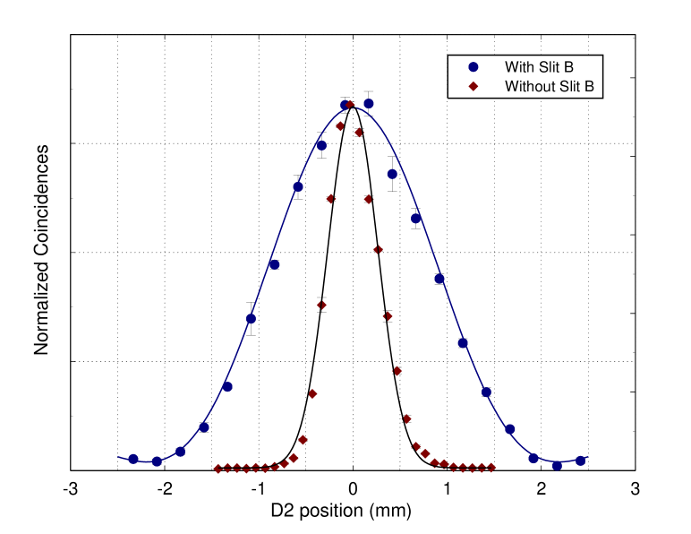
Figure 2: Results of the photon experiment by Kim and Shih, [15] aimed at realizing Popper’s proposal. The diffraction pattern in the absence of slit B (diamond symbols) is much narrower than that in the presence of a real slit (round symbols).

Let us now look at the experimental results of Kim and Shih. Equation (13) should represent the width of the observed pattern in their experiment (see Fig. 2). They observed that when the width of slit B is 0.16 mm, the width of the diffraction pattern (at half maximum) is 2 mm. When the width of slit A is 0.16 mm, but slit B is left wide open, the width of the diffraction pattern is 0.657 mm. In a Gaussian function, the full width at half maximum is related to the Gaussian width $W$ by

$$W_{fwhm}=\log(2)W$$ (14)

Using $W_{2}=0.657/\log(2)$ mm, $\lambda=702$ nm and $2L_{1}+L_{2}=2$ m, we find $\sqrt{\epsilon^{2}+\hbar^{2}/\sigma^{2}}=0.632$ mm. Assuming that a rectangular slit of width 0.16 mm corresponds to a Gaussian width $\epsilon=0.11$ mm, the number 0.632 for $\sqrt{\epsilon^{2}+\hbar^{2}/\sigma^{2}}$ is unusually large. If the number 0.632 really pertains to $\sqrt{\epsilon^{2}+\hbar^{2}/\sigma^{2}}$, it would means that the effect of imperfect correlation (represented by $\hbar/\sigma$) is much much larger than the localization effect of the slit. Clearly, something is amiss here.

A careful look reveals that the analysis we presented in the last section applies to freely evolving entangled particle, while Kim and Shih’s setup also involves a converging lens. Thus, the photons are not really free particles - their dynamics is affected by the lens. So, our next task is to incorporate the effect of the lens in our calculation.

3.2 Effect of converging lens

We assume the effect of a converging lens of focal length $f$ to be the following. If a Gaussian wave-packet of width $\sigma$ starts from a distance $2f$ from the lens, it will spread due to time evolution as it reaches the lens. The effect of lens is to have a unitary transformation on the wave-packet such that in its subsequent dynamics, it narrows instead of spreading, and comes back to its original width after a distance $2f$ from the lens. Also, the observed width of the wavepacket, immediately after emerging from the lens should be the same as that just before entering the lens. In general, we can quantify the effect of the lens by a unitary transformation of the form

$$\mathbf{U}_{f}{(\pi/2)^{-1/4}\over\sqrt{\sigma+{i\Lambda L\over\sigma}}}\exp\left({-y_{1}^{2}\over\sigma^{2}+i\Lambda L}\right) = {(\pi/2)^{-1/4}\over\sqrt{\tilde{\sigma}+{i\Lambda(L-4f)\over\tilde{\sigma}}}}$$

$$\exp\left({-y_{1}^{2}\over\tilde{\sigma}^{2}+i\Lambda(L-4f)}\right),$$

where $L$ is the distance the wave-packet, of an initial width $\sigma$, traveled before passing through the lens, and $\tilde{\sigma}$ is such that it satisfies

$$\tilde{\sigma}^{2}+{\Lambda^{2}(L-4f)^{2}\over\tilde{\sigma}^{2}}=\sigma^{2}+{\Lambda^{2}L^{2}\over\sigma^{2}}.$$ (16)

One can verify that if $L=2f$, the state emerging from the lens, given by (3.2), after traveling a further distance $2f$, assumes the form ${(\pi/2)^{-1/4}\over\sqrt{\sigma}}\exp\left({-y_{1}^{2}\over\sigma^{2}}\right)$.

Figure 3: Setup of the photon experiment by Kim and Shih, [15] aimed at realizing Popper’s proposal. Slit A is narrow while slit B is left wide open.

In this scenario, we split the time $t_{1}$, taken by particle 1 to reach slit A, into two parts: the time $t_{b1}$ taken to travel the distance $b_{1}$, from the source to the lens, and the time $t_{2f}$ taken to travel the distance $2f$, from the lens to slit A. So, the state of particle 2, after a time $t_{1}$, conditioned on particle 1 having passed through slit A, is given by

$$\phi_{2}(y_{2},t_{1}) = \int_{-\infty}^{\infty}\phi_{1}^{*}(y_{1})\psi(y_{1},y_{2},t_{1})dy_{1}$$ (17)

$$= \int_{-\infty}^{\infty}\phi_{1}^{*}(y_{1})e^{-{i\over\hbar}H_{1}t_{2f}}\mathbf{U}_{f}e^{-{i\over\hbar}H_{1}t_{b2}}e^{-{i\over\hbar}H_{2}t_{1}}\psi(y_{1},y_{2},0)dy_{1}$$

Similarly, one can write the state of particle 2 at a general time $t$, conditioned on particle 1 having passed through slit A, as

$$\phi_{2}(y_{2},t)=\int_{-\infty}^{\infty}\phi_{1}^{*}(y_{1})e^{-{i\over\hbar}H_{1}t_{2f}}\mathbf{U}_{f}e^{-{i\over\hbar}H_{1}t_{b2}}e^{-{i\over\hbar}H_{2}t}\psi(y_{1},y_{2},0)dy_{1}$$ (18)

A word of caution is needed while interpreting (18). For a time $t<t_{1}$, the two particle state is actually an entangled state, which renders any attempt to write the wave-function of just particle 2, meaningless. For such a purpose, normally one has to resort to mixed states. However, if one were to calculate any quantity, including the probability of finding particle 2 in a certain region of space, conditioned on particle 1 having passed through slit 1, (18) will give the correct result, even for a time before $t_{1}$.

For $\phi_{1}(y_{1})$ given by (5), the wave-function of particle 2, at a time $t$, has the explicit form

$$\phi_{2}(y_{2})=\exp\left({-y_{2}^{2}\over\epsilon^{2}+{\hbar^{2}\over\sigma^{2}}+i2\Lambda(b_{1}-2f)+2i\Lambda L}\right),$$ (19)

where $L$ is the distance traveled by the particle in time $t$ and $C$ is a constant necessary for normalization. For $L=2f-b_{1}$, $\phi_{2}(y_{2})$ is a Gaussian with a width equal to $\sqrt{\epsilon^{2}+\hbar^{2}/\sigma^{2}}$, which is exactly the position spread of particle 2, when it started out at the source. $L=2f-b_{1}$ corresponds to particle 2 being at slit B. Indeed, we see that because of the clever arrangement of the setup in Kim and Shih’s experiment, particle 2 is localized at slit B to a region as narrow as its initial spread. Thus, the spreading of the wave-packet because of temporal evolution, which would have been present in Popper’s original setup, has been avoided. So, in Kim and Shih’s realization, the virtual slit is indeed at the location of slit B. However, its width is larger than the width of the real slit.

Now one can calculate the width of the distribution of particle 2, as seen by detector D2. In reaching detector D2, particle 2 travels a distance $L=L_{1}+L_{2}=2f-b_{1}+L_{2}$. The width (at half maximum) of pattern at D2 is now given by

$$W_{2}=\sqrt{\epsilon^{2}+{\hbar^{2}\over\sigma^{2}}+{4\Lambda^{2}L_{2}^{2}\over\epsilon^{2}+\hbar^{2}/\sigma^{2}}}.$$ (20)

Contrasting this expression with (13), one can explicitly see the effect of introducing the lens in the experiment - basically, the length $L_{2}$ occurs here in place of $2L_{1}+L_{2}$. Using $W_{2}=0.657/\log(2)$ mm, $\lambda=702$ nm and $2L_{1}+L_{2}=2$ m, we now find $\sqrt{\epsilon^{2}+\hbar^{2}/\sigma^{2}}=0.236$ mm. Assuming that a rectangular slit of width 0.16 mm corresponds to a Gaussian width $\epsilon=0.08$ mm (which gives the correct diffraction pattern width for a real slit), we find $\hbar^{2}/\sigma^{2}=0.049~{}mm^{2}$. For a perfect EPR state, $\hbar^{2}/\sigma^{2}$ should be zero. So, we see that for a real entangled source, where correlations are not perfect, a small value of $\hbar^{2}/\sigma^{2}=0.049~{}mm^{2}$, satisfactorily explains why the diffraction pattern width is 0.657 mm, as opposed to the width of 2 mm for a real slit of the same width.

From the preceding analysis, it is clear that if $\hbar/\sigma$ were zero, the diffraction pattern would be as wide as that for a real slit. However, the smaller the quantity $\hbar/\sigma$, the more divergent is the beam. This can be seen from (4), which implies that an initial width of the beam $\Delta y_{2}=\sqrt{\Omega^{2}+\hbar^{2}/4\sigma^{2}}$, corresponds to a width $\sqrt{\Omega^{2}+{\Lambda^{2}L^{2}\over\Omega^{2}}+\hbar^{2}/4\sigma^{2}+{\Lambda^{2}L^{2}\over\hbar^{2}/\sigma^{2}}}$, after particle 2 has traveled a distance $L$. Consequently, the width of the diffraction pattern is never larger than the width of the beam, in the case of diffraction from a virtual slit. Width of the beam here refers to the width of the pattern obtained from all the counts, without any coincident counting. Thus, no additional momentum spread can ever be seen in Popper’s experiment. The conclusion is that although Kim and Shih correctly implemented Popper’s experiment through the innovative use of the converging lens, it is not decisive about Popper’s test of the Copenhagen interpretation, because of imperfect correlation between the two photons.

4 The Real Popper’s Test

The discussion in the preceding section implies that making the the correlation of the two entangled particles better, doesn’t throw any new light on the issue. However there is a way in which Popper’s test can be implemented. Popper states:[2]

“if the Copenhagen interpretation is correct, then any increase in the precision in the measurement of our mere knowledge of the particles going through slit B should increase their scatter.”

This view just says that if the (indirect) localization of particle 2 is made more precise, the momentum spread should show an increase. This could have easily been done in Kim and Shih’s experiment by gradually narrowing slit A, and observing the corresponding diffraction pattern.

An experiment which (unknowingly) implements this idea, has actually been performed, although its connection to Popper’s proposal has not been recognized. This is the so-called ghost interference experiment by Strekalov et al [20]. In the single slit ghost interference experiment, a SPDC source generates entangled photons and a single slit is put in the path of one of these. There is a lone detector D1 sitting behind the single slit, and a detector D2, in the path of the second photon, is scanned along the y direction, after a certain distance. The only way in which this experiment is different from the Popper’s proposed experiment is that D1 is kept fixed, instead of being scanned along y-axis or placed in front of a collection lens as in [15]. Now, the reason for doing coincident counting in Popper’s experiment was to make sure that only those particles behind slit B where counted, whose entangled partner passed through slit A. This was supposed to see the effect of localizing particle 1, on particle 2. In Strekalov’s experiment, all the particles counted by D2 are such that the other particle of their pair has passed through the single slit. There are many pairs which are not counted, whose one member has passed through the slit, but doesn’t reach the fixed D1. However as far as Popper’s experiment is concerned, this is not important. As long as the particles which are detected by D2 are those whose other partner passed through the slit, they will show the effect that Popper was looking for. Popper was inclined to predict that the test would decide against the Copenhagen interpretation.

Let us look at the result of Strekalov et al’s experiment (see Fig. 4). The points represent the width of the diffraction pattern, in Strekalov et al’s experiment, as a function of the slit width. For small slit width, the width of the diffraction pattern sharply increases as the slit is narrowed. This is in clear contradiction with Popper’s prediction. To emphasize the point, we quote Popper: [2]

“If the Copenhagen interpretation is correct, then such counters on the far side of slit B that are indicative of a wide scatter …should now count coincidences; counters that did not count any particles before the slit A was narrowed …”

Strekalov et al’s experiment shows exactly that, if we replace the scanning D2 by an array of fixed detectors. So, we conclude that Popper’s test has decided in favor of Copenhagen interpretation.

Figure 4: Width of the diffraction pattern, plotted against the full width of slit A. The squares represent the data of Strekalov et al’s experiment [20]. The line represents the theoretical width, calculated from (13) for $\hbar/\sigma=0.04$ mm, using the parameters of Strekalov et al’s experiment

The theoretical analysis carried out by us should apply to Strekalov et al’s experiment, with the understanding that the single slit interference pattern is seen only if D1 is fixed. In other words, if D1 were also scanned along y-axis, the diffraction pattern would essentially remain the same except that the smaller peaks, indicative of interference from different regions within the slit, would be absent. We use (13) to plot the full width at half maximum of the diffraction pattern against, $2\epsilon$, which we assume to be the full width of the rectangular slit A (see Fig 4). The plot uses $2L_{1}+L_{2}=1.8$ m, the value used in Ref. ghost, and an arbitrary $\hbar/\sigma=0.04$ mm. Our graph essentially agrees with that of Strekalov et al. Some deviation is there because we have not taken into account the beam geometry, and the finite size (0.5 mm) of the detectors, which will lead to an additional contribution to the width.

5 Discussion and conclusion

In 1987, when Collet and Loudon [7] argued that the use of a stationary source was fundamentally flawed, the general view was that Popper experiment will not be able to test the Copenhagen interpretation of quantum mechanics. Short has also emphasized that the imperfect localization is a manifestation of the problem pointed out by Collet and Loudon, and concluded that the experiment cannot implement Popper’s test [16]. Kim and Shih’s experiment actually avoids this problem by obtaining a ghost image of the slit.

We have shown that Strekalov et al’s ghost interference experiment, actually implements Popper’s test in a conclusive way, but the result is in contradiction with Popper’s prediction. It could not have been otherwise, because our theoretical analysis shows that the results are a consequence of the formalism of quantum mechanics, and not of any particular interpretation. This was also pointed out by Krips, who predicted that narrowing slit A would lead to increase in the width of the diffraction pattern behind slit B (in coincident counting) [6]. So, Krips prediction has been vindicated by Strekalov et al’s experiment.

In our view, the only robust criticism of Popper’s experiment was that by Sudbery, who pointed out that in order to have perfect correlation between the two entangled particles, the momentum spread in the initial state, had to be truly infinite, which made any talk of additional spread, meaningless [4, 5]. For some reason, the implication of Sudbery’s point was not fully understood. It is this very point which, when generalized, leads to our conclusion that no additional momentum spread in particle 2 can be seen, even in principle.

Thus, our conclusion is that although Kim and Shih’s experiment circumvents the objections raised by Collet and Loudon, it is not conclusive about Popper’s test. On the other hand, Strekalov et al’s experiment, implements Popper’s test in a conclusive way. Their results vindicate the Copenhagen interpretation of quantum mechanics (if one takes Popper’s viewpoint). In reality, the results are just a manifestation of quantum mechanics, which hardly needs any more vindication at this stage.

References

- [1] “Can quantum-mechanical description of physical reality be considered complete?”, A. Einstein, B. Podolsky, N. Rosen, Phys. Rev. 47, 777-780 (1935),
- [2] K. R. Popper, Quantum Theory and the Schism in Physics (Hutchinson, London, 1982), pp. 27–29.
- [3] “Realism in quantum mechanics and a new version of the EPR experiment”, K.R. Popper, pp. 3-25, in Open Questions in Quantum Physics, edited by G. Tarozzi and A. van der Merwe (Dordrecht, Reidel, 1985)
- [4] “Popper’s variant of the EPR experiment does not test the Copenhagen interpretation”, A. Sudbery, Phil. Sci. 52, 470–476 (1985).
- [5] “Testing interpretations of quantum mechanics”, A. Sudbery in Microphysical Reality and Quantum Formalism, edited by A. van der Merwe et al (1988) pp 267-277.
- [6] “Popper, propensities, and the quantum theory”, H. Krips, Brit. J. Phil. Sci. 35, 253–274 (1984).
- [7] “Analysis of a proposed crucial test of quantum mechanics”, M.J. Collet, R. Loudon, Nature 326, 671–672 (1987).
- [8] “Measurement-induced diffraction and interference of atoms”, P. Storey, M.J. Collet, D. F. Walls, Phys. Rev. Lett. 68, 472–475 (1992).
- [9] “Popper and the quantum theory”, M. Redhead in Karl Popper: Philosophy and Problems, edited by A. O’Hear (Cambridge, 1996) pp 163-176.
- [10] “Atomic position localization via dual measurement”, H. Nha, J.-H. Lee, J.-S. Chang, K. An, Phys. Rev. A 65, 033827–033833 (2002).
- [11] “Karl Popper and the Copenhagen interpretation”, A. Peres, Studies in History and Philosophy of Science 33, 23 (2002).
- [12] “Realism in the realized Popper’s experiment”, G. Hunter, AIP Conference Proc. 646 (1), 243–248 (2002).
- [13] “Popper’s experiment revisited”, P. Sancho, Found. Phys. 32, 789-805 (2002).
- [14] “Popper’s experiment, Copenhagen interpretation and nonlocality”, T. Qureshi, Int. J. Quant. Inf. 2, 407-418 (2004).
- [15] “Experimental realization of Popper’s experiment: violation of the uncertainty principle?”, Y.-H. Kim, Y. Shih, Found. Phys. 29, 1849–1861 (1999).
- [16] “Popper’s experiment and conditional uncertainty relations”, A. J. Short, Found. Phys. Lett. 14, 275–284 (2001).
- [17] “Understanding Popper’s experiment”, T. Qureshi, Am. J. Phys. 73, 541–544 (2005).
- [18] “Popper’s experiment and communication”, E. Gerjuoy, A.M. Sessler, Am. J. Phys. 74, 643 (2006).
- [19] “Coherence properties of entangled light beams generated by paramteric down-conversion: theory and experiment”, A. Joobeur, B. E. A. Saleh, T. S. Larchuk, M. C. Teich, Phys. Rev. A 53, 4360–4371 (1996).
- [20] “Observation of two-photon ghost interference and diffraction”, D.V. Strekalov, A.V. Sergienko, D.N. Klyshko, Y.H. Shih, Phys. Rev. Lett. 74, 3600–3603 (1995).