otangent bundle quantization: Entangling of metric and magnetic field

M. V. Karasev

Department of Applied Mathematics

Moscow Institute of Electronics and Mathematics

Moscow 109028, Russia

E-mail: karasev@miem.edu.ru

T. A. Osborn

Department of Physics and Astronomy

University of Manitoba

Winnipeg, MB, Canada, R3T 2N2

E-mail: tosborn@cc.umanitoba.ca

For manifolds $\mathcal{M}$ of noncompact type endowed with an affine connection (for example, the Levi-Civita connection) and a closed 2-form (magnetic field) we define a Hilbert algebra structure in the space $L^{2}(T^{*}\!\mathcal{M})$ and construct an irreducible representation of this algebra in $L^{2}(\mathcal{M})$. This algebra is automatically extended to polynomial in momenta functions and distributions. Under some natural conditions this algebra is unique. The non-commutative product over $T^{*}\!\mathcal{M}$ is given by an explicit integral formula. This product is exact (not formal) and is expressed in invariant geometrical terms. Our analysis reveals this product has a front, which is described in terms of geodesic triangles in $\mathcal{M}$. The quantization of $\delta$-functions induces a family of symplectic reflections in $T^{*}\!\mathcal{M}$ and generates a magneto-geodesic connection $\Gamma$ on $T^{*}\mathcal{M}$. This symplectic connection entangles, on the phase space level, the original affine structure on $\mathcal{M}$ and the magnetic field. In the classical approximation, the $\hbar^{2}$-part of the quantum product contains the Ricci curvature of $\Gamma$ and a magneto-geodesic coupling tensor.

1 Introduction

There is a well-known quantum product defined by Groenewold [1], Moyal [2], and Berezin [3] over the phase space ${\mathbb{R}}^{2n}$. This non-commutative associative product of functions corresponds to the Weyl symmetrization rule for ordering the quantum coordinates $\hat{q}^{j}$ and momenta $\hat{p}_{k}$ which obey the canonical commutation relations

$$[\hat{q}^{j},\hat{q}^{k}]=0\,,\qquad[\hat{q}^{j},\hat{p}_{k}]=i\hbar\delta^{j}_{k}\,,\qquad[\hat{p}_{j},\hat{p}_{k}]=0\,.$$ (1.1)

In the classical limit $\hbar\rightarrow 0$ this quantum product reduces to the usual product of functions over ${\mathbb{R}}^{2n}$ and yields the standard symplectic structure $dp\wedge dq$ on ${\mathbb{R}}^{2n}$.

There is also a magnetic analog [4, 5] of this quantum product, where $\hat{p}$ plays the role of the kinetic momenta and satisfies the commutation relations

$$[\hat{q}^{j},\hat{q}^{k}]=0\,,\qquad[\hat{q}^{j},\hat{p}_{k}]=i\hbar{\delta^{j}_{k}}\,,\qquad[\hat{p}_{j},\hat{p}_{k}]=i\hbar{F_{kj}}(\hat{q})\,.$$ (1.2)

Here $F$ is the Faraday tensor (the strength of the magnetic field for $n=3$). The small $\hbar$ asymptotics of this product generates the ‘magnetic’ symplectic structure on ${\mathbb{R}}^{2n}$

$$\omega=dp\wedge dq+\frac{1}{2}F(q)\,dq\wedge dq\,.$$ (1.3)

The magnetic algebra generated by relations (1.2) is an interesting and useful object for physical and mathematical applications, [6–15]. In particular, the case of quadratic magnetic field $F$ represents an example of quadratic quantum algebra (1.2) which corresponds to the symplectic space ${\mathbb{R}}^{2n}$ of constant non-zero curvature [5]. Also it is useful to recall that the form of relations (1.2) is gauge invariant, i.e. it does not depend on the choice of magnetic potential, and so all the calculations in this algebra are gauge-independent a priori.

One would like to examine what happens in this framework if the flat $q$-space ${\mathbb{R}}^{n}$ is replaced by a curved manifold $\mathcal{M}$. This means that the Euclidean metric on ${\mathbb{R}}^{n}$ is replaced by a Riemannian metric, or more generally, by an affine connection $\Gamma$ on $\mathcal{M}$. Accordingly, the phase space ${\mathbb{R}}^{2n}$ is replaced by the cotangent bundle $T^{*}\!\mathcal{M}$.

The fundamental question arises: how to define a quantum product over $T^{*}\!\mathcal{M}$ which would naturally generalize the products appearing in the Euclidean cases (1.1) and (1.2) and incorporate the connection $\underline{\Gamma}$ on $\mathcal{M}$?

This is an old quantization problem, which was posed by Dirac [16] and Mackey [17] and initially studied in [18–24] and other works.

The recent mathematical investigation of this problem has been carried out in [25–33] including the case where the metric and the magnetic field are both present on $\mathcal{M}$ [25, 26, 33]. There is also a large literature, beginning with the paper by Widom [34], where this problem was studied from the perspective of pseudodifferential and Fourier integral operators.

In spite of certain essential progress, there remain many significant open questions in this problem area.

First, we note that the papers cited above do not address the following questions:

How does the connection $\underline{\Gamma}$ entangle with the magnetic field $F$ on $\mathcal{M}$ via the quantization process? Are $\underline{\Gamma}$ and $F$ combined in a natural geometrical way?

This family of questions closely parallels the issues raised in Weyl’s discovery of the gauge principle. In the paper [35] Weyl constructed a connection on the configuration space which combined the Levi-Civita metric connection with the magnetic potential and was ‘gauge’ invariant. Subjected to Einstein’s criticism [36] that the construction was incompatible with physical reality, Weyl revised the direction of his program (and soon invented the beginnings of modern gauge theory). Nevertheless we now think that Weyl’s original intention finds very strong support in the quantization theory where one has a natural opportunity to extend configuration space $\mathcal{M}$ to the phase space $T^{*}\!\mathcal{M}$ and re-examine the ‘connection problem’ therein.

Secondly, although all the works dealing with the quantization problem over $T^{*}\!\mathcal{M}$ use more or less the same core idea for generalizing the Groenewold–Moyal product (just replace in the phase functions all the straight chords by geodesics) there is a wide variation in the definition of the amplitude functions. This variety of amplitudes illustrates the known phenomena of the non-uniqueness of quantization.

Even in the Euclidean example an aspect of this non-uniqueness is present, and correlates, for instance with the ordering problem, cf. [37, 38, 4]. In the Euclidean case, conditions which uniquely identify the Groenewold–Moyal product and Weyl ordering are known [39–41]; in the context of formal deformation theory see the discussion in [42–44]. The main idea in all these approaches is to exploit certain symmetry group actions. For inhomogeneous manifolds $\mathcal{M}$ this is not possible. So, the question remains open: How to select a unique quantization on $\mathcal{M}$?

Thirdly, one may claim that in the literature there is still no explicit formula for the quantum product over $T^{*}\!\mathcal{M}$, even for the simplest examples of curved manifolds $\mathcal{M}$, even with no magnetic field.

We mean here an exact formula, not a formal deformation one. Such an exact formula could be applied, for instance, to highly oscillating or singularly concentrated (as $\hbar\rightarrow 0$) functions on $T^{*}\!\mathcal{M}$ which are required to describe Schrödinger quantum dynamics or eigenfunction problems on $\mathcal{M}$. On this topic we recall the asymptotic quantization theory [45] which allows this type of ‘semiclassical’ $\hbar$-dependence in its symbols and deals with symplectic manifolds of general type without having a global polarization. However for symplectic manifolds, $\prec\!\!T^{*}\!\mathcal{M},\omega\!\!\succ$, it is natural to ask more: namely to obtain an exact, not semiclassical, quantization formula which is globally and geometrically stated on $T^{*}\!\mathcal{M}$.

In this paper we present solutions to these questions in the case where the configuration manifold $\mathcal{M}$ is geodesically simply connected. As an example one can take $\mathcal{M}$ to be a symmetric Riemannian manifold of noncompact type, say, the hyperboloid in the Minkowski space and, in particular, the Lobachevski plane. Another class of examples is given by manifolds $\mathcal{M}\approx{\mathbb{R}}^{n}$ whose metric is a deformation of the Euclidean one.

Part of the results described below can also be applied to generic curved manifolds $\mathcal{M}$, for instance to compact manifolds.

The magnetic field $F$ can be an arbitrary closed 2-form on $\mathcal{M}$.

By using the averaging of $F$ along geodesics we define symplectic transformations of the phase space $\prec\!\!T^{*}\!\mathcal{M},\omega\!\!\succ$ which correspond to autoparallel vector fields on $\mathcal{M}$. This is a magneto-geodesic analog of the Gallilei translations in ${\mathbb{R}}^{n}$. We introduce unitary operators in $L^{2}(\mathcal{M})$ corresponding to these symplectic transformations and exploit them to select in a unique way the quantization operation

$$f\rightarrow\hat{f}$$ (1.4)

on a function space over $T^{*}\!\mathcal{M}$ (Sect. 3).

The mapping (1.4) determines an exact irreducible representation of the Hilbert algebra $L^{2}(T^{*}\!\mathcal{M})$ in the Hilbert space $L^{2}(\mathcal{M})$. We also extend this mapping to a wider algebra which includes, in particular, functions on $T^{*}\!\mathcal{M}$ polynomial in momenta, some exponential highly oscillating functions as $\hbar\rightarrow 0$, delta functions, etc. Note that we are employing here the Hilbert algebra approach to quantization theory. If one examines the $C^{*}$-algebra corresponding to our quantum Hilbert algebra over $T^{*}\!\mathcal{M}$ then it is of the strict quantization type [46].

At the next stage in Sect. 4, we analyze which symplectic transformations $\sigma_{x}$ of the phase space $\prec\!\!T^{*}\!\mathcal{M},\omega\!\!\succ$ correspond to the quantum $\delta$-functions, $\widehat{\delta}_{x}$. In this way a family of magneto-geodesic reflections on the space $T^{*}\!\mathcal{M}$ is obtained. They are the phase space analogs of the geodesic reflections in $\mathcal{M}$ interacting with the magnetic field.

In Sect. 5 we use the related $\sigma$-reflective curves to represent the quantum product $\star$ over $T^{*}\!\mathcal{M}$ which corresponds to the quantization operation (1.4) in the usual way

$$\hat{f}\,\hat{g}=\widehat{f{\star}\,g}\,.$$ (1.5)

The product $\star$ is given by an exact, explicit and geometrically invariant integral formula (5.16).

This formula can be used for different subalgebras of functions over $T^{*}\mathcal{M}$. Being restricted to the subalgera of polynomial in momenta functions, this formula works for the case of a generic affine manifold $\mathcal{M}$ (possibly not geodesically simply connected).

In Sect. 6 we prove that the asymptotic expansion of the exact quantum product as $\hbar\rightarrow 0$ has the following form

$$f\,{\star}\,g=fg-\frac{i\hbar}{2}f\langle\overleftarrow{\nabla}\Psi\overrightarrow{\nabla}\rangle g-\frac{\hbar^{2}}{8}f\Big{[}\langle\overleftarrow{\nabla}\Psi\overrightarrow{\nabla}\rangle^{2}+3\langle\overleftarrow{\nabla}\Psi\mathcal{R}\Psi\overrightarrow{\nabla}\rangle\Big{]}g+O(\hbar^{3})\,.$$ (1.6)

Here $\Psi=\big{[}\begin{array}[]{cc}0&-I\\ I&F\end{array}\big{]}$ is the Poisson tensor on $T^{*}\!\mathcal{M}$ associated with the symplectic structure (1.3), $\nabla$ denotes the covariant derivative corresponding to a symplectic connection $\Gamma$ on $\prec\!\!T^{*}\!\mathcal{M},\omega\!\!\succ$ defined by magneto-geodesic reflections, cf. (6.5) and $\mathcal{R}$ is the Ricci tensor of this connection. The phase space covariant derivative $\nabla$ appearing in the asymptotic expansion (1.6) matches our quantization formulas with the deformation quantization [18, 22, 28, 29, 42, 47–50]. In the deformation quantization framework the symplectic connection corresponding to a given star product is determined by the $\hbar^{2}$-term via a formula like (1.6).

In our approach the connection $\Gamma$ is derived in a different way, via $\sigma$-reflections. In Sect. 6 the explicit formulas are obtained for the connection $\Gamma$ and for its curvature in terms of $\underline{\Gamma}$  and $F$. These formulas entangle the configuration space data $\underline{\Gamma}$  and $F$ on the phase space level. We call $\Gamma$ a magneto-geodesic connection.

The part of $\Gamma$ which depends on the magnetic field $F$ we call a magneto-geodesic coupling. This is a 3-tensor on $\mathcal{M}$. In the case of a Riemannian manifold $\mathcal{M}$ with a Levi-Civita connection $\underline{\nabla}$ this tensor is equivalent to the one which arises in the inhomogeneous Maxwell equation (with current and charge).

The preprint version of this paper is found in arXiv: quant-ph/0505144.

2 Preliminary Definitions and Notation

After von Neumann [51], Wigner [52], Groenewold [1], and Stratonovich [53] it was understood that the basic object of the quantization theory is a Hilbert algebra together with its exact irreducible representation in a Hilbert space.

By definition (see, for instance, in [54]) the Hilbert algebra $\mathcal{L}$ is a complete linear space with three structures: an associative product $\star\,$, a scalar product $(\cdot,\cdot)$, and an involution ^∗, which are mutually consistent.

Let $\mathcal{H}$ be a Hilbert space. Then the minimal Hilbert algebra which has an irreducible representation in $\mathcal{H}$ is the algebra of all Hilbert–Schmidt operators on $\mathcal{H}$.

The basic idea of quantization theory is to replace the operator algebra by a function algebra over an appropriate phase space. Following the Correspondence Principle one is taking $\mathcal{H}$ to be

$$\mathcal{H}=L^{2}(\mathcal{M},dm)\,,$$

where $\mathcal{M}$ is a configuration space, i.e. a smooth manifold with a smooth positive measure $dm$. The phase space is then defined as $T^{*}\!\mathcal{M}$, i.e. the cotangent bundle over $\mathcal{M}$, and the Hilbert algebra is assumed to be

$$\mathcal{L}=L^{2}(T^{*}\!\mathcal{M},dl)\,.$$

Here $dl$ is the normalized Liouville measure

$$dl(x)=\frac{dx}{(2\pi\hbar)^{n}}\,,\qquad dx=dq^{1}\cdots dq^{n}dp_{1}\cdots dp_{n}\,,$$

where $x=(q,p)\,,\,q\in\mathcal{M}\,,\,p\in T^{\star}_{q}\mathcal{M}\,,\,n={\rm\,{dim}}\,\mathcal{M}$. So, the scalar product in the algebra $\mathcal{L}$ is given by

$$(f,g)=\frac{1}{(2\pi\hbar)^{n}}\int_{T^{*}\!\mathcal{M}}f(x)\,\overline{g(x)}\,dx\,,$$

and the involution is given by the complex conjugation

$$f^{*}=\overline{f}\,.$$

In addition to the scalar product there is the trace functional

$$\mbox{\rm tr}\,(f)\equiv\frac{1}{(2\pi\hbar)^{n}}\int_{T^{*}\!\mathcal{M}}f(x)\,dx$$

where $f\in L^{1}(T^{*}\!\mathcal{M},dl)$. We ask that the product in the algebra $\mathcal{L}$ obey the following property: the ideal $\mathcal{L}^{1}\equiv\mathcal{L}{\star}\,\mathcal{L}$ is a subset of $L^{1}(T^{*}\!\mathcal{M},dl)$, and

$$\mbox{\rm tr}\,(f{\star}\,\overline{g})=(f,g)$$ (2.1)

for any $f,g\in\mathcal{L}$.

The representation of the algebra $\mathcal{L}$ in the Hilbert space $\mathcal{H}$ is denoted by

$$f\rightarrow\hat{f}$$ (2.2)

and is assumed to satisfy the usual axioms

$$\hat{f}^{\dagger}=\widehat{\overline{f}}\,,\qquad\hat{f}\,\hat{g}=\widehat{f{\star}\,g}\,,\qquad\mbox{\rm Tr}\,(\hat{f})=\mbox{\rm tr}\,(f)\,.$$ (2.3)

Here Tr indicates the operator trace and ${\dagger}$ the adjoint. The last axiom is restricted to the subspace $\mathcal{L}^{1}$.

The inverse to the mapping (2.2) is called dequantization or symbol mapping

$$\hat{f}\rightarrow f={\mathrm{Smb}}(\hat{f})\,.$$

It is convenient to write the quantization mapping (2.2) in the integral form

$$\hat{f}\,=\int_{T^{*}\!\mathcal{M}}f(x)\,\Delta_{x}\,dx\,,$$ (2.4)

where $\{\Delta_{x}\}$ is a family of operators in $\mathcal{H}$ parameterized by points $x\in T^{*}\!\mathcal{M}$. Then the symbol mapping is given by

$$f(x)=(2\pi\hbar)^{n}\,\mbox{\rm Tr}\,(\hat{f}\,\Delta_{x})\,.$$ (2.5)

The first and third axioms in (2.3), together with (2.1), as well as the definition (2.4) together with (2.5) are reformulated in terms of the operator family $\Delta$ as follows

$$\Delta_{x}^{\dagger}=\Delta_{x}\,,\quad(2\pi\hbar)^{n}\,\mbox{\rm Tr}\,(\Delta_{x}\Delta_{y})=\delta_{x}(y)\,,\quad(2\pi\hbar)^{n}\int_{T^{*}\!\mathcal{M}}\Delta_{x}\otimes\Delta_{x}\,dx=\mathcal{I}\,.$$ (2.6)

Here $\delta$ is the Dirac delta-function with respect to the canonical measure on $T^{*}\!\mathcal{M}$ and $\mathcal{I}$ is the antipodal operator $\psi\otimes\chi\rightarrow\chi\otimes\psi$ on Hilbert space $\mathcal{H}\otimes\mathcal{H}$.

The second axiom in (2.3) reads

$$(f\,{\star}\,g)(x)=\int_{T^{*}\!\mathcal{M}}\int_{T^{*}\!\mathcal{M}}K_{\star}(x,y,z)\,f(y)\,g(z)\,dy\,dz$$ (2.7)

where the distribution $K_{\star}$ is defined as

$$K_{\star}(x,y,z)=(2\pi\hbar)^{n}\,\mbox{\rm Tr}\,(\Delta_{x}\Delta_{y}\Delta_{z})\,.$$ (2.8)

Of course, in formulas (2.4)–(2.8) appropriate care must be taken with respect to the convergence of integrals and traces (using the weak topology and a suitable distribution extension of functions). For instance, the distribution character of $\mbox{\rm Tr}\,(\Delta_{x}\Delta_{y})$ and $\mbox{\rm Tr}\,(\Delta_{x}\Delta_{y}\Delta_{z})$ is defined by first integrating the operator-valued functions with $C_{0}^{\infty}$ test functions and after that computing the trace.

Various symmetry properties follow directly from the definition of $K_{\star}$ in (2.8): it is invariant under any cyclic permutation of its arguments, and it obeys $K_{\star}\rightarrow\overline{K_{\star}}$ under the permutation of any pair of its arguments.

The family $\Delta$ was introduced by Stratonovich [53] for the case $\mathcal{M}={\mathbb{R}}^{n}$. In [55] such a family was called a quantizer. See also details and examples in [56–60].

One can call the last two quantizer properties in (2.6) orthonormality and operator completeness, respectively. The identities in (2.6) imply that quantization (2.4) and dequantization (2.5) are mutually consistent.

In the next section we construct the quantizer using the affine connection and the magnetic field on $\mathcal{M}$, and then apply formulas (2.7), (2.8) to calculate the quantum product over $T^{*}\!\mathcal{M}$.

But before that, we need to demonstrate how the ${\star}$ product can be extended to other classes of symbols beyond the algebra $\mathcal{L}$.

Let $\mathcal{F}$ be any subalgebra in $\mathcal{L}$. Denote by $\mathcal{F}^{\prime}$ the space of linear functionals on $\mathcal{F}$. Employing the canonical measure we identify functionals with distributions on $T^{*}\!\mathcal{M}$ via

$$\langle f,h\rangle=\int_{T^{*}\!\mathcal{M}}f(x)\,h(x)\,dx\,,\qquad f\in\mathcal{F}^{\prime}\,,h\in\mathcal{F}\,.$$

Obviously $\mathcal{F}\subset\mathcal{F}^{\prime}$. Further note that $\mathcal{F}^{\prime}$ is an $\mathcal{F}$-module, i.e. $f\in\mathcal{F}^{\prime}\,,\,k\in\mathcal{F}\quad\Rightarrow\quad f\,{\star}\,k\in\mathcal{F}^{\prime}\,,\,\,k\,{\star}\,f\in\mathcal{F}^{\prime}$ where by definition

$$\langle f\,{\star}\,k,h\rangle\stackrel{{\scriptstyle\mathrm{def}}}{{=}}\langle f,k\,{\star}\,h\rangle\,,\qquad\langle k\,{\star}\,f,h\rangle\stackrel{{\scriptstyle\mathrm{def}}}{{=}}\langle f,h\,{\star}\,k\rangle\,,\qquad\forall\,h\in\mathcal{F}\,.$$ (2.9)

Denote by $\mathcal{F}_{\star}$ the following subset

$$\mathcal{F}_{\star}=\{f\in\mathcal{F}^{\prime}|\,f{\star}\,h\in\mathcal{F}\,\,{\mathrm{and}}\,\,h\,{\star}\,f\in\mathcal{F}\,,\,\,\forall\,h\in\mathcal{F}\}\,.$$

In particular, $\mathcal{F}\subset\mathcal{F}_{\star}$ .

We call $\mathcal{F}$ a normal subalgebra if the set $\mathcal{F}_{\star}$ obeys the property

$$\langle f,h\,{\star}\,g\rangle=\langle g,f\,{\star}\,h\rangle\,,\qquad\forall\,f,g\in\mathcal{F}_{\star}\,,\quad\forall\,h\in\mathcal{F}\,.$$ (2.10)

If $\mathcal{F}$ is a normal subalgebra in $\mathcal{L}=L^{2}(T^{*}\!\mathcal{M})$, then the set $\mathcal{F}_{\star}$ is endowed with the algebra structure

$$\langle f{\star}\,g,h\rangle\stackrel{{\scriptstyle\mathrm{def}}}{{=}}\langle f,g\,{\star}\,h\rangle\,,\qquad\forall\,f,g\in\mathcal{F}_{\star}\,,\quad\forall\,h\in\mathcal{F}\,,$$ (2.11)

which is consistent with the involution $\overline{f\,{\star}\,g}=\overline{g}\,{\star}\,\overline{f}\,.$

Verification of the embedding $f\star g\in\mathcal{F}_{\star}$ and the $\star$-associativity is achieved by repeated applications of (2.9)–(2.11) in combination with the associativity of $\mathcal{F}$. The algebra $\mathcal{F}_{\star}$ is a natural extension of the subalgebra $\mathcal{F}$.

Note that the unity function $1$ does not belong to $\mathcal{F}$ or $\mathcal{L}$, but is automatically an element of $\mathcal{F}_{\star}$ and $1\,{\star}\,f=f\,{\star}\,1=f\,,\ \forall\,f\in\mathcal{F}_{\star}\,.$ So, $\mathcal{F}_{\star}$ is an involutive algebra with unity.

In the next section we introduce a concrete example of a normal subalgebra $\mathcal{F}\subset\mathcal{L}$ and its extension $\mathcal{F}_{*}$ suitable for quantizing the phase space $T^{*}\!\mathcal{M}$. In the case $\mathcal{M}={\mathbb{R}}^{n}$ similar extensions were used in [15, 61–64].

3 Quantization and dequantization over $T^{*}\!\mathcal{M}$

Let $\mathcal{M}$ be a smooth oriented manifold with an affine torsion free connection $\underline{\Gamma}$ and a smooth positive measure $dm$.

We assume that $\mathcal{M}$ is geodesically simply connected, that is, every pair of points is connected by a unique geodesic, and moreover this geodesic is infinitesimally isolated (has no conjugate points).

For any $q\in\mathcal{M}$ we use the notations

$$V_{q} = {\underline{\exp}}_{\ q}^{-1}\,,\qquad s_{q}={\underline{\exp}}_{\ q}(-V_{q})\,,\hfill$$

$$j_{q} = 2^{-n}|\det\big{(}\partial V_{q}+\partial V_{q}(s_{q})\big{)}|\,,\qquad\partial V_{q}\equiv\frac{\partial V_{q}}{\partial q}\,,\phantom{\bigg{(}}$$

$$J_{q} = j_{q}\,\frac{\mathcal{D}m(s_{q})}{\mathcal{D}m}\,,\qquad e_{q}\equiv\frac{\mathcal{D}m({\underline{\exp}}_{\ q}(v))}{\mu(q)\mathcal{D}v}\,\bigg{|}_{v=V_{q}}\,.$$

In these formulas one has the following objects:

• the exponential map ${\underline{\exp}}_{\ q}:T_{q}\mathcal{M}\rightarrow\mathcal{M}$ which is everywhere non-degenerate,

• for any $q^{\prime}\in\mathcal{M}$ the vector $V_{q}(q^{\prime})\in T_{q}\mathcal{M}$ is the velocity on the geodesic connecting $q$ with $q^{\prime}$ in unit time,

• the mapping $s_{q}:\mathcal{M}\rightarrow\mathcal{M}$ is the geodesic reflection about point $q$, ${s_{q}}^{2}={id}$ ,

• the Jacobian $j_{q}\in C^{\infty}(\mathcal{M})$ is invariant under the reflection $s_{q}$ ,

• $\mu>0$ denotes the density of the measure on $\mathcal{M}$, so that $dm(q)=\mu(q)\,dq$ ,

• the Jacobian $\mathcal{D}m(s_{q})/\mathcal{D}m\in C^{\infty}(\mathcal{M})$ is obtained by transforming the measure $dm$ under the diffeomorphism $s_{q}$ ,

• the Jacobian $e_{q}\in C^{\infty}(\mathcal{M})$ determines the transformation of the measure $dm$ under the diffeomorphism ${\underline{\exp}}_{\ q}$ .

In addition, let $F$ be a closed 2-form on $\mathcal{M}$. We fix an arbitrary point $o\in\mathcal{M}$ and define the function $\Phi_{q}\in C^{\infty}(\mathcal{M})$ as

$$\Phi_{q}(q^{\prime})=\int_{\pi_{q}(q^{\prime})}F\,.$$ (3.1)

Here $\pi_{q}(q^{\prime})$ is a two-dimensional surface in $\mathcal{M}$ whose oriented boundary is composed of three geodesics (Fig. 1): the geodesic from $q^{\prime}$ to $o$, from $o$ to $s_{q}(q^{\prime})$, and from $s_{q}(q^{\prime})$ back to $q^{\prime}$. The values of the function $\Phi_{q}$ are just the magnetic flux through the surfaces $\pi_{q}$.

Figure 1: Geodesic triangle $\pi_{q}(q^{\prime})$ in $\mathcal{M}$.

Now we are ready to define the quantizer $\{\Delta_{x}|\,x\in T^{*}\!\mathcal{M}\}$. This family of operators is determined by its integral kernels $\Delta_{x}(a,b)$

$$(\Delta_{x}\psi)(a)=\int_{\mathcal{M}}\Delta_{x}(a,b)\,\psi(b)\,dm(b)\,,\qquad\psi\in\mathcal{D}(\mathcal{M})\,.$$

Here and below we denote by $\mathcal{D}(\mathcal{N})\equiv C_{0}^{\infty}(\mathcal{N})$ the space of all compactly supported $C^{\infty}$-functions on a manifold $\mathcal{N}$.

Let $x=(q,p)$, so that $p\in T^{*}_{q}\mathcal{M}$. We set

$$\Delta_{x}(a,b)\stackrel{{\scriptstyle\mathrm{def}}}{{=}}\frac{1}{(\pi\hbar)^{n}}\sqrt{J_{q}(a)}\exp\Big{\{}\frac{i}{\hbar}\big{(}2p\,V_{q}(a)+\Phi_{q}(a)\big{)}\Big{\}}\,\delta_{s_{q}(a)}(b)\,,$$ (3.2)

where $\delta$ is the delta-function on $\mathcal{M}$ with respect to the measure $dm$; the product $p\,V_{q}(a)$ represents the natural pairing of the covector $p$ and the tangent vector $V_{q}(a)$ in $T_{q}\mathcal{M}$.

Lemma 1.

The family of operators $\{\Delta_{x}\}$ defined by the integral kernels (3.2) obeys properties (2.6) and so is a quantizer :

$$\begin{array}[]{c}{\displaystyle{\overline{\Delta_{x}(a,b)}=\Delta_{x}(b,a)\,,}}\\ {\displaystyle{(2\pi\hbar)^{n}\int_{\mathcal{M}}\int_{\mathcal{M}}\Delta_{x}(a,b)\,\Delta_{y}(b,a)\,dm(a)\,dm(b)=\delta_{x}(y)\,,}}\phantom{\Bigg{(}}\\ {\displaystyle{(2\pi\hbar)^{n}\int_{T^{*}\!\mathcal{M}}\Delta_{x}(a,b)\,\Delta_{x}(c,d)\,dx=\delta_{a}(d)\,\delta_{b}(c)\,.}}\end{array}$$ (3.3)

The proof follows directly from the definition (3.2) by simple computation of integrals containing delta-functions.

For some manifolds $\mathcal{M}$ the function $j_{q}$ may be unbounded. In this case the quantizer $\Delta_{x}$ is an unbounded operator but remains selfadjoint with domain $\mathcal{D}(\Delta_{x})=\{\psi\in\mathcal{H}\,|\int j_{q}|\psi|^{2}\,dm\ <\infty\}$. The family $\{\Delta_{x}\}$ and all $x$-derivatives are strongly continuous on $\mathcal{D}(\mathcal{M})$.

Recall that the operators $\hat{f}$ are defined by formula (2.4). Let $\mathfrak{F}$ denote the integral kernel of the operator $\hat{f}$,

$$(\hat{f}\psi)(a)=\int_{\mathcal{M}}\mathfrak{F}(a,b)\,\psi(b)\,dm(b)\,,\qquad\psi\in\mathcal{D}(\mathcal{M})\,.$$ (3.4)

For simplicity we assume that $\mathfrak{F}\in\mathcal{D}(\mathcal{M}\times\mathcal{M})$.

Applying formula (2.5), one obtains the analog of the Wigner transform.

Lemma 2.

The symbol $f$ is constructed from the kernel $\mathfrak{F}$ via

$$f(q,p)=\int_{T_{q}\mathcal{M}}e^{\textstyle{-iup/\hbar}}\,\big{(}k\mathfrak{F}\big{)}\big{(}{\underline{\exp}}_{\ q}({\frac{u}{2}})\,,{\underline{\exp}}_{\ q}(-\frac{u}{2})\big{)}\,\mu(q)\,du\,.$$ (3.5)

Here the function $k$ is given by

$$k(a,b)\stackrel{{\scriptstyle\mathrm{def}}}{{=}}\Big{(}j_{a\vee b}(a)\,e_{a\vee b}(a)\,e_{a\vee b}(b)\Big{)}^{1/2}\,\exp\Big{\{}\textstyle{-i\Phi_{a\vee b}(a)/\hbar}\Big{\}}\,,$$ (3.6)

and $a\vee b$ denotes the geodesic midpoint (Fig. 2), that is

$$s_{a\vee b}(a)=b\,.$$ (3.7)

The inverse transform from symbol to kernel results from (2.4). Denote the Fourier image of $f$ in the momentum variable by

$$f^{\sim}(q,u)\stackrel{{\scriptstyle\mathrm{def}}}{{=}}\frac{1}{(2\pi\hbar)^{n}}\int_{T_{q}^{\star}\mathcal{M}}e^{\textstyle{iup/\hbar}}\,f(q,p)\,\frac{dp}{\mu(q)}\,.$$ (3.8)

Lemma 3.

The integral kernel $\mathfrak{F}$ of the operator corresponding to the symbol $f\in\mathcal{D}(T^{*}\mathcal{M})$, is given by

$$\mathfrak{F}(a,b)=\frac{f^{\sim}(a\vee b,a\wedge b)}{k(a,b)}\,,$$ (3.9)

where $a\vee b$ is the geodesic midpoint (3.7) and $a\wedge b$ is the geodesic velocity at the midpoint (Fig. 2)

$$a\wedge b\stackrel{{\scriptstyle\mathrm{def}}}{{=}}V_{a\vee b}(a)-V_{a\vee b}(b)=2\,V_{a\vee b}(a)\,.$$ (3.10)

In the flat case $\mathcal{M}={\mathbb{R}}^{n}$ one has $|k(a,b)|=1$ and (3.5), (3.9) becomes the standard Wigner transform in the presence of a magnetic field.

Using (3.9) one can readily compose the product of two operators and find a simple composition rule in terms of Fourier-imaged symbols. To formulate the result let us recall that the tangent bundle $T\mathcal{M}$ is endowed with a natural groupoid multiplication [27]

$$n^{\prime},n^{\prime\prime}\mapsto n^{\prime}\circ n^{\prime\prime}$$ (3.11)

by means of the left and right (target and source) mappings

$$\tilde{l}:T\mathcal{M} \rightarrow \mathcal{M}\,,\quad\tilde{l}(n)\stackrel{{\scriptstyle\mathrm{def}}}{{=}}{\underline{\exp}}_{\ q}(\frac{u}{2})\,,$$

$$\tilde{r}:T\mathcal{M} \rightarrow \mathcal{M}\,,\quad\tilde{r}(n)\stackrel{{\scriptstyle\mathrm{def}}}{{=}}{\underline{\exp}}_{\ q}(-\frac{u}{2})\,,\quad n\equiv(q,u)\in T\mathcal{M}\,.$$

Namely, the product (3.11) of two elements $n^{\prime},n^{\prime\prime}\in T\mathcal{M}$ is well determined iff $\tilde{r}(n^{\prime})=\tilde{l}(n^{\prime\prime})$, and in this case one has $\tilde{l}(n^{\prime}\circ n^{\prime\prime})=\tilde{l}(n^{\prime})\,,\,\tilde{r}(n^{\prime}\circ n^{\prime\prime})=\tilde{r}(n^{\prime\prime})$. Note that the mappings $\tilde{l},\tilde{r}$ themselves can be expressed in terms of the groupoid multiplication as

$$\tilde{l}(n)=n\circ n^{-1}\,,\qquad\tilde{r}(n)=n^{-1}\circ n\,,$$

where $n^{-1}\equiv(q,-u)$ is the element inverse to $n$ in $T\mathcal{M}$.

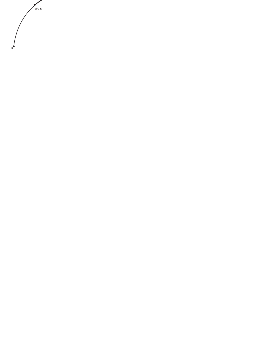
Figure 2: Geodesic mid-point and velocity in $\mathcal{M}$.

Lemma 4.

Composition of Fourier–imaged symbols over $T\mathcal{M}$ is given by the groupoid modified convolution

$$\big{(}f^{\sim}\odot g^{\sim}\big{)}(n)=\int_{n=n^{\prime}\circ n^{\prime\prime}}\frac{\kappa(n)}{\kappa(n^{\prime})\kappa(n^{\prime\prime})}\,f^{\sim}(n^{\prime})\,g^{\sim}(n^{\prime\prime})\,dm\,.$$ (3.12)

Here $n,n^{\prime},n^{\prime\prime}$ are points from $T\mathcal{M}$, the function $\kappa(n)\equiv k(\tilde{l}(n),\tilde{r}(n))$ is given by (3.6) and by the left and right mappings of the groupoid structure (3.11). The integration in (3.12) is taken with respect to the measure $dm\big{(}\tilde{r}(n^{\prime})\big{)}=dm\big{(}\tilde{l}(n^{\prime\prime})\big{)}$ over the manifold $\mathcal{M}$.

Formula (3.12) belongs to the class of Connes’ type tangential groupoid quantization formulas [27, 31, 4]. Note that in the convolution integrand (3.12) we have an additional groupoid cocycle

$$C(n^{\prime},n^{\prime\prime})=\frac{\kappa(n^{\prime}\circ n^{\prime\prime})}{\kappa(n^{\prime})\kappa(n^{\prime\prime})}=|C(n^{\prime},n^{\prime\prime})|\,\exp\left\{\frac{i}{\hbar}\int_{\Delta(n^{\prime},n^{\prime\prime})}F\right\}\,.$$ (3.13)

The cocycle property

$$C(n,m\circ l)\,C(m,l)=C(n\circ m,l)\,C(n,m)$$ (3.14)

guaranties the associativity of the modified groupoid convolution (3.12).

The phase of the cocycle (3.13) is just the magnetic flux through the triangle $\Delta(n^{\prime},n^{\prime\prime})$ in $\mathcal{M}$ bounded by geodesics (Fig. 3) with mid-points $q,q^{\prime},q^{\prime\prime}$ and mid-velocities $u,u^{\prime},u^{\prime\prime}$ such that

$$n^{\prime}=(q^{\prime},u^{\prime}),\qquad n^{\prime\prime}=(q^{\prime\prime},u^{\prime\prime}),\qquad n^{\prime}\circ n^{\prime\prime}=(q,u)\,.$$

This phase is similar to its form in the Euclidean case [4], but now it also senses the non-Euclidean connection on $\mathcal{M}$. On the phase space level the property (3.14) is equivalent to the Stokes theorem applied to the geodesic tetrahedron in $\mathcal{M}$ with sides corresponding to elements $n,m,l,m\circ l,n\circ m,l\circ n,n\circ m\circ l\in T\mathcal{M}$.

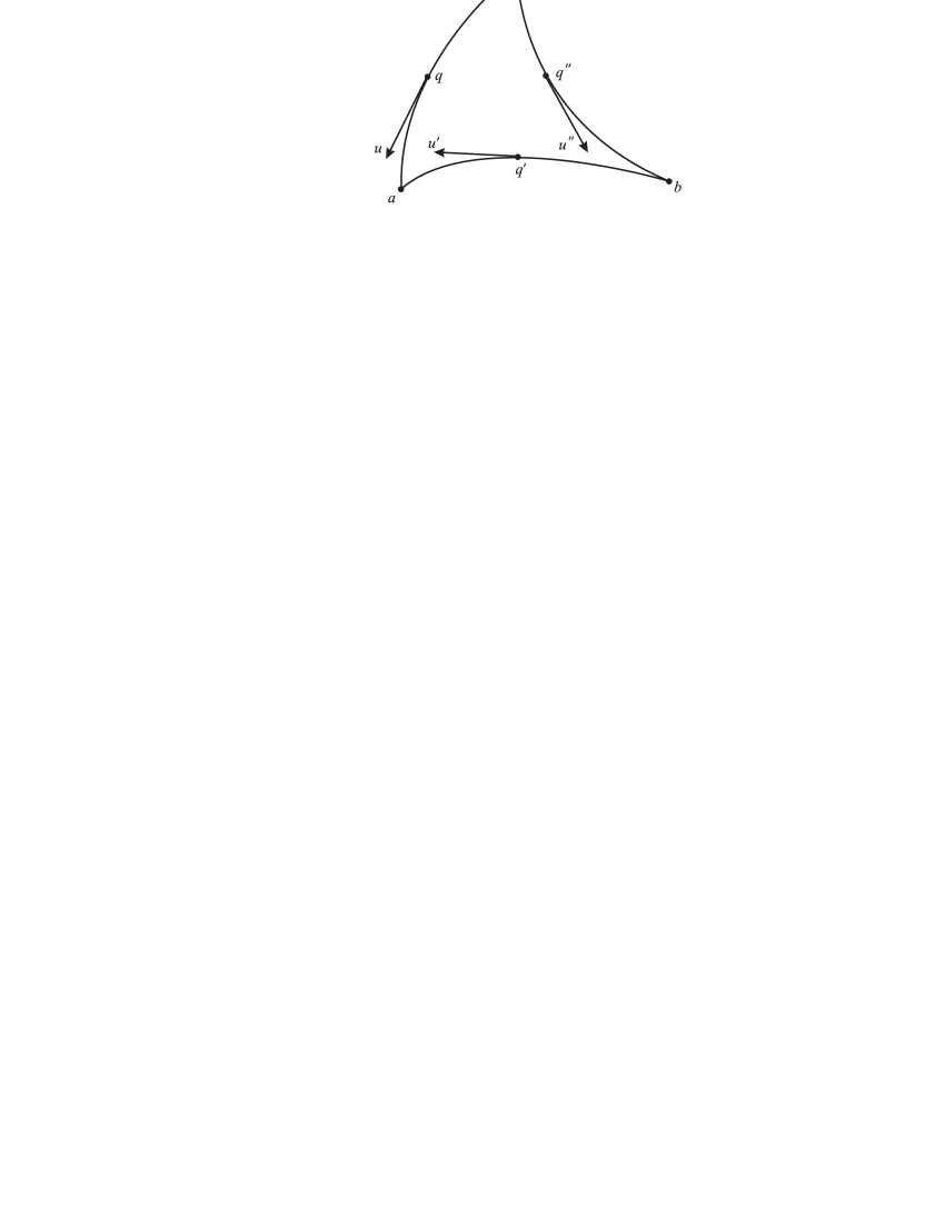
Figure 3: Geodesic triangle in $\Delta(n^{\prime},n^{\prime\prime})$ in $\mathcal{M}$.

The amplitude $C(n^{\prime},n^{\prime\prime})$ of the cocycle (3.13) obtained from (3.6) is

$$|C(n^{\prime},n^{\prime\prime})|=\left({\frac{j_{q}(c)}{j_{q^{\prime}}(a)\,j_{q^{\prime\prime}}(b)}}\cdot\frac{e_{q}(a)e_{q}(c)}{e_{q^{\prime}}(a)e_{q^{\prime}}(b)e_{q^{\prime\prime}}(b)e_{q^{\prime\prime}}(c)}\right)^{1/2}\,.$$

This amplitude is an additional ‘geodesic’ contribution to the groupoid cocycle structure (3.13).

Obviously, one has the following

Proposition 1.

The quantization mapping $f\rightarrow\hat{f}$, defined by (3.4), (3.9) is an isomorphism between the algebra $\mathcal{L}=L^{2}(T^{*}\!\mathcal{M},dl)$ and the algebra of all Hilbert–Schmidt operators acting on the Hilbert space $\mathcal{H}=L^{2}(\mathcal{M},dm)$. The quantum product $\star$ in the algebra $\mathcal{L}$ is generated by the groupoid modified convolution (3.12), as follows

$$\big{(}f{\star}\,g\big{)}^{\sim}=f^{\sim}\odot g^{\sim}\,.$$ (3.15)

Now we would like to extend the quantization mapping to a wider algebra.

Examining formula (3.12) one can easily see that the class $\mathcal{D}(T\mathcal{M})$ is invariant with respect to the $\odot$ convolution. Moreover, the class of $C^{\infty}$-functions on $TM$ with compact support in tangential directions is a $\mathcal{D}(T\mathcal{M})$-module with respect to this convolution. Thus one is led to the following definitions.

Denote by $\mathcal{F}=\mathcal{F}(T^{*}\!\mathcal{M})$ the space of functions on $T^{*}\!\mathcal{M}$ whose momentum Fourier image belongs to $\mathcal{D}(T\mathcal{M})$.

Further, denote by $\mathcal{P}=\mathcal{P}(T^{*}\!\mathcal{M})$ the space of $C^{\infty}$ functions on $T^{*}\!\mathcal{M}$ which are polynomial in momenta. Let $\mathcal{P}^{l}\subset\mathcal{P}$ be the subspace which consists of polynomials of degree $l$ in momenta.

From the above discussion and the definitions of Sect. 2 we have

Proposition 2.

$\mathcal{F}$ is a normal subalgebra of the Hilbert algebra $\mathcal{L}=L^{2}(T^{*}\!\mathcal{M})$.

Proposition 3.

The space $\mathcal{P}$ is an involutive subalgebra in $\mathcal{F}_{\star}$ with the gradation:
$\mathcal{P}^{l}{\star}\,\mathcal{P}^{m}\subset\mathcal{P}^{l+m}$. The commutator in the algebra $\mathcal{P}$ is graded as follows

$$[\mathcal{P}^{l},\mathcal{P}^{m}]_{\star}\subset\mathcal{P}^{l+m-1}\,,\qquad l,m\geq 0\,,$$ (3.16)

where $\mathcal{P}^{-1}\equiv 0$. In particular, $[\mathcal{P}^{0},\mathcal{P}^{0}]_{\star}=0$.

For any $f\in\mathcal{F}_{\star}$ the operator

$$\hat{f}:\mathcal{D}(\mathcal{M})\rightarrow\mathcal{D}^{\prime}(\mathcal{M})$$ (3.17)

is defined by its bilinear form

$$(\hat{f}\psi,\chi)_{\mathcal{H}}=\langle f,\rho_{\psi|\chi}\rangle\,.$$ (3.18)

Here $\rho_{\psi|\chi}$ is the Wigner function

$$\rho_{\psi|\chi}(x)\stackrel{{\scriptstyle\mathrm{def}}}{{=}}(\Delta_{x}\psi,\chi)_{\mathcal{H}}\,.$$ (3.19)

It is evident that $\rho_{\psi|\chi}\in\mathcal{F}$ if $\psi,\chi\in\mathcal{D}(\mathcal{M})$  and so the ‘matrix elements’ (3.18) are well-defined. In the particular case where $f\in\mathcal{F}$ this definition of the operator $\hat{f}$ coincides with the above definition (3.4), (3.9).

As one would expect, the Wigner function obeys the usual probability interpretation together with the associated bound condition

$$\int_{T^{*}_{q}\mathcal{M}}\rho_{\psi|\psi}(q,p)\,dp=|\psi(q)|^{2}\,,\quad|\rho_{\psi|\psi}(q,p)|\leq{\frac{1}{(\pi\hbar)^{n}}}\int_{\mathcal{M}}(j_{q})^{1/2}|\psi|^{2}dm\,.$$

Lemma 5.

If $f\in\mathcal{P}$ then $\hat{f}$ maps $\mathcal{D}(\mathcal{M})$ into $\mathcal{D}(\mathcal{M})$; moreover, it is a differential operator. If $f\in\mathcal{P}^{l}$ then $\hat{f}$ is a differential operator of order $l$.

Let us consider now some basic examples of functions from $\mathcal{F}_{\star}$ or $\mathcal{P}$ and the operators (3.17) corresponding to them.

Example 1.

Let $1$ be the unit function on $T^{*}\!\mathcal{M}$. Then $1\in\mathcal{F}_{\star}$ and $\hat{1}=I$ is the identity operator in $L^{2}(\mathcal{M},dm)$.

Let $\delta_{x}$ be the delta-function on $T^{*}\!\mathcal{M}$ concentrated at the point $x$. Then $\delta_{x}\in\mathcal{F}_{\star}$. The corresponding operator is the quantizer (3.2),

$$\widehat{\phantom{,}\delta_{x}}=\Delta_{x}\,.$$

In the Euclidean case see [56, 57].

Example 2.

Let $f\in\mathcal{P}^{1}$. Then $f$ is represented by the sum $f(q,p)=\varphi(q)+f_{W}(q,p)$ with $\varphi\in C^{\infty}(\mathcal{M})$, $f_{W}(q,p)=p\,W(q)$, and where $W$ is a vector field on $\mathcal{M}$. Obviously $\widehat{\varphi}=\varphi$ (the multiplication operator) and

$$\widehat{f_{W}}=-i\hbar\,(W+\frac{1}{2}\,{\mathrm{div}}\,W)-A^{o}\,W\,.$$ (3.20)

Here on the right hand side the field $W$ is considered as a first order differential operator, and div $W$ denotes the divergence of $W$ with respect to the measure $dm$. The function $A^{o}\,W$ in (3.20) is the pairing of the vector field $W$ with the 1-form $A^{o}$ on $\mathcal{M}$, and $A^{o}$ is a primitive of the Faraday 2-form, i.e.

$$dA^{o}=F\,.$$

This 1-form is uniquely determined by the radial gauge condition that $A^{o}(q)$ is perpendicular to the velocity of the geodesic connecting $o$ with $q$;

$$A^{o}(q)\,V_{q}(o)=0\,.$$ (3.21)

An explicit formula for $A^{o}$ is the following [65]

$$A^{o}(q)=\int_{o}^{q}\left({\frac{\partial Q}{\partial q}}\right)^{*}F(Q)\,dQ\,,$$ (3.22)

where $Q$ is the geodesic from $o$ to $q$, and the integral (3.22) is taken along this geodesic. The magnetic potential (3.22) can be interpreted as the average of the Lorentz force $F(Q)\,\dot{Q}$ with respect to the Jacobi field along the geodesic.

At this stage it is useful to discuss the relationship between various gauge choices and structure of the quantizer. The definition (3.2) of $\Delta_{x}$ makes no reference to any particular magnetic potential. However the magnetic phase flux $\Phi_{q}$, when written as a line integral, is expressed in terms of the radial gauge by

$$\Phi_{q}(a)=\int_{s_{q}(a)}^{a}A^{o}\,.$$ (3.23)

Here the integral is taken along the geodesic on $\mathcal{M}$ connecting $b\!=\!s_{q}(a)$ to $a$. The $a\,o$ and $o\,b$ geodesic contributions to $\Phi_{q}(a)$ vanish by virtue of the radial gauge condition (3.21). The Examples 2 and 3 demonstrate the dependence on just this special radial gauge 1-form $A^{o}$. If one modifies the definition of the quantizer by replacing $A^{o}$ in (3.23) by a magnetic vector potential in some other gauge, say $A$, then the potential $A$ will replace $A^{o}$ in the quantization of the momentum coordinate, (3.20). We conclude that although the quantum algebra is gauge invariant, its representation depends on the gauge choice.

In the Euclidean case $\mathcal{M}={\mathbb{R}}^{n}$ the 1-form (3.22) coincides with the Valatin potential [66], and condition (3.21) is the Dirac gauge condition (see details in [4]).

Example 3.

Let $M$ be a covariantly constant bivector field on $\mathcal{M}$ and $f_{M}(q,p)\!\equiv\!M^{jk}(q)p_{j}p_{k}$ $\forall p\in T^{*}_{q}\mathcal{M}$. Then $f_{M}\in\mathcal{P}^{2}$ and

$$\widehat{f_{M}}=(-i\hbar\underline{\nabla}_{j}-A^{o}_{j})\,M^{jk}\,(-i\hbar\underline{\nabla}_{k}-A^{o}_{k})\,,$$

where $\underline{\nabla}$ is the covariant derivative defined by the connection $\underline{\Gamma}$ on $\mathcal{M}$, and $A^{o}_{j}$ are components of the 1-form (3.22).

In particular, let $\Gamma$ be the Levi-Civita connection , and $g=(\!(g_{jk})\!)$ be the metric tensor on $\mathcal{M}$. Then

$$\widehat{g^{jk}(q)p_{j}p_{k}}=g^{jk}(-i\hbar\underline{\nabla}_{j}-A^{o}_{j})\,(-i\hbar\underline{\nabla}_{k}-A^{o}_{k})\,.$$

If the magnetic field is absent this reduces to $-\hbar^{2}\triangle$ (the Laplace operator on $\mathcal{M}$).

Example 4.

Let $W$ be a vector field on $\mathcal{M}$, and $r\in C^{\infty}(\mathcal{M})$. Consider the function on $T^{*}\!\mathcal{M}$ given by

$$r_{W}(q,p)\equiv r(q)\exp\Big{\{}{\frac{i}{\hbar}}p\,W(q)\Big{\}}\,,\qquad p\in{T^{*}}_{q}\mathcal{M}\,.$$ (3.24)

Suppose the following condition holds:

$${\mathit{the\,matrix}}\,\,\frac{1}{2}\partial W(b)/\partial b{[\partial V_{a}(b)/\partial b]}^{-1}\,\,{\mathit{has\,no\,eigenvalues\,\pm 1\,for\,any\,}}a,b\in\mathcal{M}\,.$$ (3.25)

Then $r_{W}\in\mathcal{F}_{\star}$.

Indeed, by computing ${r_{W}}^{\sim}$ and transforming this to the kernel form (3.9) one obtains the delta-function $\delta\big{(}W(a\vee b)+a\wedge b\big{)}$, which must be a well-defined distribution in both $a$ and $b$ (in order to achieve the embedding $r_{W}\in\mathcal{F}_{\star}$). Thus it is sufficient to assume that both determinants

$$\det\,{\frac{\partial}{\partial a}}\big{(}W(a\vee b)+a\wedge b\big{)}\neq 0,\qquad\det\,{\frac{\partial}{\partial b}}\big{(}W(a\vee b)+a\wedge b\big{)}\neq 0\,,$$ (3.26)

are non-zero for all $a,b\in\mathcal{M}$. This is equivalent to condition (3.25).

The operator corresponding to the symbol $r_{W}$, subject to the condition (3.25), acts in $\mathcal{H}$ as

$$(\widehat{r_{W}}\psi)(a)={\frac{J_{q}\big{(}{\underline{\exp}}_{\ q}(-\frac{1}{2}W(q))\big{)}^{1/2}}{\Big{|}\det\big{(}\partial V_{q}(a)+\frac{1}{2}\partial W(q)\big{)}\Big{|}}}\,r(q)e^{\textstyle{-i\Phi_{q}(a)/\hbar}}\,\psi\big{(}{\underline{\exp}}_{\ q}({\textstyle{\frac{1}{2}}}W(q))\big{)}\bigg{|}_{q=Q(a)}$$ (3.27)

where $Q(a)$ is the solution of the equation

$${\underline{\exp}}_{\ Q}\big{(}{\textstyle{-\frac{1}{2}}}W(Q)\big{)}=a\,.$$ (3.28)

Now, consider the specific class of autoparallel vector fields, i.e. those satisfying the identity

$$\underline{\nabla}_{W}W=0\qquad{\mathrm{o}r}\qquad W^{j}\partial_{j}W^{k}+\underline{\Gamma}_{js}^{k}W^{j}W^{s}=0\,.$$

In this case the flow $R^{t}:\mathcal{M}\rightarrow\mathcal{M}$ of the field $W$ is given by

$$R^{t}(q)={\underline{\exp}}_{\ q}\big{(}t\,W(q)\big{)}\,.$$ (3.29)

Note that condition (3.25) is satisfied automatically and equation (3.28) now reads
$R^{-1/2}(Q)=a$, and so, $Q(a)=R^{1/2}(a)$.

Moreover, ${\underline{\exp}}_{\ q}\big{(}\frac{1}{2}W(q)\big{)}=\exp_{a}\big{(}W(a)\big{)}$ and so $\psi({\underline{\exp}}_{\ q}\big{(}\frac{1}{2}W(q)\big{)}\big{|}_{q=Q(a)}\!=\psi(R^{1}(a))$.

Thus the operator $\widehat{r_{W}}$ acts as a shift operator along the trajectories of the field $W$.

Lemma 6.

Let $W$ be an autoparallel vector field on $\mathcal{M}$, generating the flow (3.29). Set

$$r^{t}(q)\stackrel{{\scriptstyle\mathrm{def}}}{{=}}\det\,DV_{q}(R^{t/2}(q))\left(\frac{\det\,dR^{t/2}(q)\cdot\det\,dR^{-t/2}(q)}{j_{q}\big{(}R^{t/2}(q)\big{)}}\right)^{1/2}.$$ (3.30)

Then the family

$$\widehat{r_{W}^{t}}\equiv\widehat{r^{t}\exp\big{\{}\frac{it}{\hbar}f_{W}\big{\}}}\qquad(t\in{\mathbb{R}})\,,$$ (3.31)

where $f_{W}(q,p)\equiv pW(q)$, forms a one-parameter group of unitary operators in $\mathcal{H}$ acting by the formula

$$\big{(}\widehat{r_{W}^{t}}\psi\big{)}(a)=\sqrt{\frac{\mathcal{D}m\big{(}R^{t}(a)\big{)}}{\mathcal{D}m(a)}}\exp\left\{\frac{i}{\hbar}\int_{\pi^{t}(a)}F\right\}\,\psi\big{(}R^{t}(a)\big{)}\,.$$ (3.32)

Here the boundary of a surface $\pi^{t}(a)\subset\mathcal{M}$ is composed of three geodesics connecting the points $o\rightarrow R^{t}(a)\rightarrow a\rightarrow o$.

Indeed the operator given by (3.32) is automatically unitary. So, to prove the lemma we just need to compare formulas (3.32) and (3.27), and choose an appropriate amplitude function $r$.

Note that the mapping $R^{t}:\mathcal{M}\rightarrow\mathcal{M}$ can be naturally lifted up to the mapping

$$\gamma_{W}^{t}:T^{*}\!\mathcal{M}\rightarrow T^{*}\!\mathcal{M}\,,\qquad\gamma_{W}^{t}\left(\begin{array}[]{c}q\\ p\end{array}\right)=\left(\begin{array}[]{l}R^{t}(q)\\ {dR^{t}(q)}^{-1*}(p+\beta^{t})\end{array}\right)\,.$$ (3.33)

Here the covector $\beta^{t}\in T^{*}_{q}\mathcal{M}$ is defined by $\beta^{t}=A(q,R^{t}(q))$, where

$$A(q,a)\stackrel{{\scriptstyle\mathrm{def}}}{{=}}\int_{a}^{q}\left({\frac{\partial Q}{\partial q}}\right)^{*}F(Q)\,dQ\,.$$ (3.34)

The potential $A(q,a)\in T_{q}^{*}\mathcal{M}$ is the version of (3.22) with the initial point $a$ instead of $o$: $d_{q}\,A(q,a)=F(q),\,\,A(q,a)V_{q}(a)=0$. In particular, if $a=o$, then $A(q,o)\equiv A^{o}(q)$ in the notation of (3.22).

Corollary 1.

Let $W$ be an autoparallel vector field on $\mathcal{M}$, and $g\in\mathcal{P}^{1}$. Then the following permutation formula holds on the dense domain $\mathcal{D}(\mathcal{M})\subset\mathcal{H}$

$$\widehat{r^{t}_{W}}\cdot\widehat{g}\cdot{\widehat{r^{t}_{W}}}^{-1}=\widehat{g^{t}_{W}}\,,\qquad g_{W}^{t}\stackrel{{\scriptstyle\mathrm{def}}}{{=}}{\gamma_{W}^{t}}^{*}g\,.$$ (3.35)

Thus we see that the unitary operators $\widehat{r^{t}_{W}}$ with symbols of exponential type (3.31) play the role of the quantum transformations corresponding to the classical symplectic transformations $\gamma_{W}^{t}$ (3.33). Permutation formula (3.35) belongs to the general class of Fock-type formulas [67] which relate classical symplectic transformations to quantum unitary operators (see also in [38, 45, 64]).

Properties (3.16) and (3.35) which we derived form the definition of the quantizer (3.2) actually determine the quantization uniquely.

Proposition 4.

If a quantization obeys the axioms (2.6) and the graded commutator property (3.16), and if for any autoparallel vector field $W$ on $\mathcal{M}$ there is a function $r^{t}\in C^{\infty}(\mathcal{M})$ such that the operator $\widehat{r_{W}^{t}}$ (3.31) is unitary and the property (3.35) holds, then this quantization coincides with the one defined by (3.5), (3.9).

These conditions for uniqueness are, in a sense, analogous to those known in the Euclidean case with no magnetic field [39–41], but our Proposition 4 uses different logical assumptions.

We call the quantization defined by (3.5), $(\ref{III.11})$ a magneto-geodesic quantization.

Observe that if the form of the quantizer kernel is a priori assumed to be of the type (3.2) having the phase and $\delta$-function structure given there but with unknown amplitude, then requiring that $\Delta_{x}$ obey axioms (2.6) fixes the amplitude. The additional properties (3.16), (3.35) in Proposition 4 were introduced to uniquely select the $\delta$-function and the phase function of (3.2).

Note that in the case $F=0$ (no magnetic field) the quantization which we uniquely identify above, should coincide with the one suggested in [31]. Our formulas (3.5), (3.9) in this case are similar to formulas (7) from [31], but a non-trivial recalculation of the Jacobian in the cochain (3.6) is required in order to bring it into the form used in [31].

Comparison of our quantization formulas (3.5), (3.9) with the versions introduced in [19, 23, 25, 26, 28, 30, 33] shows a difference in the amplitude factor $k$ of (3.6) and this corresponds with the fact that the last two axioms in (2.6) do not hold for those other quantizations.

4 Magneto-geodesic reflections

The magneto-geodesic quantization defined in the previous section is based on the quantizer structure. We now analyze this structure from the viewpoint of symplectic transformations in the phase space $\prec\!\!T^{*}\!\mathcal{M},\omega\!\!\succ$.

First note that the quantizer $\Delta_{x}$ can be decomposed into the product of its unitary part $\stackrel{{\scriptstyle\circ}}{{\Delta}}_{x}$ and its modulus $|\Delta_{x}|$ as follows

$$\Delta_{x}=|\Delta_{x}|\,\cdot\stackrel{{\scriptstyle\circ}}{{\Delta}}_{x}\,,$$ (4.1)

where $x=(q,p)\in T^{*}\!\mathcal{M}$. Here $|\Delta_{x}|$ is the positive square root of $\Delta_{x}^{\dagger}\Delta_{x}=\Delta_{x}^{2}$. It has the form of a multiplication operator $|\Delta_{x}|=(\pi\hbar)^{-n}\sqrt{j}_{q}$. The unitary part $\stackrel{{\scriptstyle\circ}}{{\Delta}}_{x}$ is

$$\stackrel{{\scriptstyle\circ}}{{\Delta}}_{x}=\sqrt{\frac{\mathcal{D}m(s_{q})}{\mathcal{D}m}}\,\exp\left\{{\frac{2i}{\hbar}}p\,V_{q}+{\frac{i}{\hbar}}\Phi_{q}\right\}\,s_{q}^{*}\,,$$ (4.2)

where $s_{q}^{*}$ is the operator in $\mathcal{H}=L^{2}(\mathcal{M},dm)$ generated by the geodesic reflection

$$(s^{*}_{q}\psi)(q^{\prime})=\psi\big{(}s_{q}(q^{\prime})\big{)}\,,\qquad\psi\in\mathcal{H}\,.$$

One can continue this decomposition and represent $\stackrel{{\scriptstyle\circ}}{{\Delta}}_{x}$ as the product of two unitary factors

$$\stackrel{{\scriptstyle\circ}}{{\Delta}}_{x}=E_{x}\cdot T_{x}\,,$$ (4.3)

which are defined by

$$E_{x}\equiv\exp\left\{{\frac{2i}{\hbar}}p\,V_{q}+{\frac{i}{\hbar}}\Phi_{q}\right\}\,,\qquad T_{x}\equiv\sqrt{\frac{\mathcal{D}m(s_{q})}{\mathcal{D}m}}\,s_{q}^{*}\,.$$ (4.4)

Note that both $E_{x}$ and $T_{x}$ are unitary and they both commute with $|\Delta_{x}|$. In addition, $T_{x}$ and $\stackrel{{\scriptstyle\circ}}{{\Delta}}_{x}$ are self-adjoint.

Now we would like to associate the unitary factors in (4.3) with symplectic transformations of phase space. This is achieved by means of a Fock procedure like (3.35).

Proceed first with the operator $T_{x}$. For each $x=(q,p)\in T^{*}\!\mathcal{M}$ define the transformation $t_{x}$ of the phase space by the following formula:

$$t_{x}\left(\begin{array}[]{c}q^{\prime}\\ p^{\prime}\end{array}\right)=\left(\begin{array}[]{l}s_{q}(q^{\prime})\phantom{\Big{)}}\\ ds_{q}(q^{\prime})^{-1*}\big{(}p^{\prime}+\beta_{q}(q^{\prime})\big{)}\end{array}\right)\,.$$ (4.5)

Here $q^{\prime}$ runs over $\mathcal{M},\,\,p^{\prime}\in T^{*}_{q^{\prime}}\mathcal{M}$, and the 1-form $\beta_{q}$ on $\mathcal{M}$ is determined by

$$\beta_{q}=A^{o}-s_{q}^{*}A^{o}\,,$$ (4.6)

where $A^{o}$ is the 1-form (3.22) and $s_{q}^{*}$ denotes the pullback of a 1-form. Obviously the mapping $t_{x}$ preserves the form $\omega$ (1.3).

Lemma 7.

For any $g\in\mathcal{P}^{1}$ the permutation formula

$$T_{x}\,\hat{g}\,T_{x}^{-1}=\widehat{t_{x}^{*}\,g}$$ (4.7)

holds on the dense domain $\mathcal{D}(\mathcal{M})\subset\mathcal{H}$.

Formula (4.7) is easily derived from (3.20) and (4.5). It relates the unitary operator $T_{x}$ in the Hilbert space $\mathcal{H}=L^{2}(\mathcal{M},dm)$ to the symplectic transformation $t_{x}$ on the phase space $\prec\!\!T^{*}\!\mathcal{M},\omega\!\!\succ$.

Now we proceed in the same way with the operator $E_{x}$. For each $x=(q,p)\in T^{*}\!\mathcal{M}$ let us define the transformation $e_{x}$ of phase space as follows

$$e_{x}\left(\begin{array}[]{c}q^{\prime}\\ p^{\prime}\end{array}\right)=\left(\begin{array}[]{l}q^{\prime}\phantom{\Big{)}}\\ p^{\prime}-2\,dV_{q}(q^{\prime})^{*}p-d\Phi_{q}(q^{\prime})\end{array}\right)\,.$$ (4.8)

Here $dV_{q}$ is the differential of the mapping $V_{q}=\underline{\exp}_{\,q}^{-1}$. This transformation preserves the form $\omega$.

Lemma 8.

For any $g\in\mathcal{P}^{1}$ the permutation formula

$$E_{x}\,\hat{g}\,E_{x}^{-1}=\widehat{e_{x}^{*}\,g}$$ (4.9)

holds on the dense domain $\mathcal{D}(\mathcal{M})\subset\mathcal{H}$.

This formula relates the unitary $E_{x}$ with the symplectic $e_{x}$ and follows without difficulty from (3.20) and (4.4).

As a consequence of these calculations we have

$$\stackrel{{\scriptstyle\circ}}{{\Delta}}_{x}\,\hat{g}\,{\stackrel{{\scriptstyle\circ}}{{\Delta}}_{x}^{-1}}=E_{x}\,T_{x}\,\hat{g}\,T_{x}^{-1}E_{x}^{-1}=\widehat{e_{x}^{*}\,t_{x}^{*}\,g}\,,$$

for any $g\in\mathcal{P}^{1}$. Thus one obtains the composition of two symplectic transformations

$$\sigma_{x}\stackrel{{\scriptstyle\mathrm{def}}}{{=}}t_{x}\circ e_{x}\,.$$ (4.10)

Corollary 2.

The symplectic transformations $\{\sigma_{x}\}$ are related to the unitary part of the quantizer by the identity

$$\stackrel{{\scriptstyle\circ}}{{\Delta}}_{x}\,\widehat{g}\,\stackrel{{\scriptstyle\circ}}{{\Delta}}_{x}^{-1}=\widehat{\sigma_{x}^{*}\,g}\,,$$ (4.11)

for any $g\in\mathcal{P}^{1}$, and any $x\in T^{*}\!\mathcal{M}$. These identities hold on the dense domain $\mathcal{D}(\mathcal{M})\subset\mathcal{H}$ .

From formulas (4.5), (4.8) and from the equalities

$$d\Phi_{q}(q^{\prime})=\beta_{q}(q^{\prime})-\alpha_{q}(q^{\prime})\,,\qquad\alpha_{q}(q^{\prime})\stackrel{{\scriptstyle\mathrm{def}}}{{=}}A\big{(}q^{\prime},q\big{)}-ds_{q}(q^{\prime})^{*}A(s_{q}(q^{\prime}),q)\,,$$ (4.12)

the symplectic mapping $\sigma_{x}$ is determined to be

$$\sigma_{x}\left(\begin{array}[]{c}q^{\prime}\\ p^{\prime}\end{array}\right)=\left(\begin{array}[]{l}s_{q}(q^{\prime})\phantom{\Big{)}}\\ ds_{q}(q^{\prime})^{-1*}\big{[}p^{\prime}-2\,dV_{q}(q^{\prime})^{*}p+\alpha_{q}(q^{\prime})\big{]}\end{array}\right)\,.$$ (4.13)

Here the potential $A$ is given by (3.34). Note the potential $A$ and thereby the right hand side above is gauge independent although (4.5) and (4.8) are gauge dependent (they depend on a choice of the point $o$ in the potential $A^{o}$ in (3.22)).

Let us check the simplest properties of the family of mappings (4.13). If the running point $x^{\prime}=(q^{\prime},p^{\prime})$ coincides with $x$, then $\sigma_{x}(x^{\prime})|_{x^{\prime}=x}=x$. Thus the point $x$ is a fixed point of the transformation $\sigma_{x}$.

Furthermore, from the evident quantum permutation relations

$$T_{x}\,E_{x}=E_{x}^{-1}\,T_{x}\,,\qquad T_{x}^{2}=I$$

one obtains the corresponding classical counterparts

$$e_{x}\circ t_{x}=t_{x}\circ e_{x}^{-1}\,,\qquad t_{x}^{2}=id\,.$$

The definition (4.10) then implies

$$\sigma_{x}^{2}=t_{x}\circ e_{x}\circ t_{x}\circ e_{x}=t_{x}\circ t_{x}\circ e_{x}^{-1}\circ e_{x}=id\,.$$

Thus Corollary 2 can be completed as follows.

Corollary 3.

The family $\{\sigma_{x}\,|\,x\in T^{*}\!\mathcal{M}\}$ of symplectic transformations on the space $\prec\!\!T^{*}\!\mathcal{M},\omega\!\!\succ$ is given by formula (4.13) and possesses the properties:

• $x$ is a unique and isolated fixed point of $\sigma_{x}$ ,

• each $\sigma_{x}$ is a reflection, i.e. $\sigma_{x}^{2}=id$ .

This family of reflections can be considered as a lift to $T^{*}\!\mathcal{M}$ of the family of reflections $\{s_{x}\}$ given on $\mathcal{M}$. We call $\sigma_{x}$ a magneto-geodesic reflection. The maps $\{\sigma_{x}\}$ generalize the family of magnetic reflections found in [5] for the phase space $\prec\!\!T^{*}{\mathbb{R}}^{n},\omega\!\!\succ$ with the Euclidean connection on $\mathcal{M}={\mathbb{R}}^{n}$. Now our reflections (4.13) combine both: a nontrivial magnetic field and a nontrivial affine connection on $\mathcal{M}$.

We note that the correspondence between the quantizer and the phase space reflections was observed in [56] for the Euclidean space ${\mathbb{R}}^{2n}=T^{*}{\mathbb{R}}^{n}$ with no magnetic field, see also [57, 58]. In this latter case the reflections are just $\sigma_{x}(x^{\prime})=2x-x^{\prime}\,.$

In the general phase space $T^{*}\!\mathcal{M}$ by using the magneto-geodesic reflections $\sigma_{x}$ one can easily define the notions of $\sigma$-midpoints and $\sigma$-reflective curves.

Namely, the point $x\in T^{*}\!\mathcal{M}$ is called a $\sigma$-midpoint between $x^{\prime},x^{\prime\prime}\in T^{*}\!\mathcal{M}$ if $x^{\prime\prime}=\sigma_{x}(x^{\prime})$. From (4.13) it follows that any two points from $T^{*}\!\mathcal{M}$ have a unique $\sigma$-midpoint.

A continuous curve passing through a point $x\in T^{*}\mathcal{M}$ is called $\sigma$-reflective with respect to $x$ if it consists of pairs of points with the midpoint $x$. The projection of the $\sigma$-reflective curve from $T^{*}\!\mathcal{M}$ onto $\mathcal{M}$ is a reflective curve in $\mathcal{M}$, and vice versa, any reflective curve from $\mathcal{M}$ (in particular, the geodesic) can be lifted to a $\sigma$-reflective curve on $T^{*}\!\mathcal{M}$ (but of course, not uniquely).

5 Integral formula for quantum product

Next we present an explicit formula for the product $f\star g$, expressed directly in terms of the functions $f$ and $g$. The definition of $\star$ product was given in (3.15). In principle, one could use (3.15) to compute $f\star g$. But it is convenient to use the equivalent representation (2.7).

First we compute the distribution (2.8), that is the trace of the composition of three quantizers $\Delta_{x}\Delta_{y}\Delta_{z}$. Label the phase space points here by

$$x=(a,\xi),\,y=(b,\eta),\,z=(c,\zeta),\quad{\mathrm{where}}\,\,\xi\in T_{a}^{*}\mathcal{M},\,\eta\in T_{b}^{*}\mathcal{M},\zeta\in T_{c}^{*}\mathcal{M}.$$ (5.1)

Let $(q,q^{\prime})$ denote the two arguments of the integral kernel of the composition $\Delta_{x}\Delta_{y}\Delta_{z}$. Employing (3.2) gives

$$(2\pi\hbar)^{n}\cdot{\mathrm{Kernel}}\big{(}\Delta_{x}\Delta_{y}\Delta_{z}\big{)}(q,q^{\prime})=T_{a,b,c}^{\xi,\eta,\zeta}(q)\,\delta_{s_{c}s_{b}s_{a}(q)}(q^{\prime})\,,\phantom{\bigg{)}}$$ (5.2)

$$T_{a,b,c}^{\xi,\eta,\zeta}(q)=(\pi\hbar)^{-2n}\exp\left\{S_{a,b,c}^{\xi,\eta,\zeta}\right\}\,\varphi_{a,b,c}(q)\,.\qquad\,\quad$$ (5.3)

The phase and amplitude functions in (5.3) are

$$S_{a,b,c}^{\xi,\eta,\zeta}(q)=2\left[\xi V_{a}(q)+\eta V_{b}\big{(}s_{a}(q)\big{)}+\zeta V_{c}\big{(}s_{b}s_{a}(q)\big{)}\right]\,+\Phi_{a}(q)+\Phi_{b}(s_{a}(q))+\Phi_{c}(s_{b}s_{a}(q))\,,$$ (5.4)

$$\varphi_{a,b,c}(q)=2^{n}\,\big{[}J_{a}(q)\,J_{b}(s_{a}(q))\,J_{c}(s_{b}s_{a}(q))\big{]}^{1/2}\,.\qquad\,\quad\phantom{\bigg{)}}$$ (5.5)

Clearly, $T_{a,b,c}^{\xi,\eta,\zeta}(q)$ is a non-singular, continuous function of all its arguments.

The integral kernel (5.2) is singular. Therefore, in order to evaluate the trace of the corresponding operator, we first contract the distribution (5.2) with a test function $\phi\in\mathcal{D}(\mathcal{M})$ by the parameter $c\in\mathcal{M}$. This computation is implemented by using the formula

$$\int_{\mathcal{M}}\delta_{s_{c}s_{b}s_{a}(q)}(q^{\prime})\,\phi(c)\,dm(c)=\phi(c)\,{\bigg{|}\frac{\mathcal{D}m(s_{c}s_{b}s_{a}(q))}{\mathcal{D}m(c)}}\bigg{|}^{-1}_{\,c=q^{\prime}\vee s_{b}s_{a}(q)}\,.$$ (5.6)

On the right hand side of this formula the point $c$ is taken to be the mid-point $q^{\prime}\vee s_{b}s_{a}(q)$, (see Fig. 4).

Figure 4: Mapping $s_{c}s_{b}s_{a}(q)=q^{\prime}$.

In order to evaluate the trace we have to put $q=q^{\prime}$ and integrate over all $q\in\mathcal{M}$. Thus from (5.2), (5.6) one obtains

$$(2\pi\hbar)^{n}\!\int_{\mathcal{M}}\!\mbox{\rm Tr}\left(\Delta_{(a,\xi)}\,\Delta_{(b,\eta)}\,\Delta_{(c,\zeta)}\right)\,\phi(c)\,dm(c)=\int_{\mathcal{M}}\!T_{a,b,c}^{\xi,\eta,\zeta}(q)\frac{\phi(c)}{\big{|}{\frac{\mathcal{D}m(s_{c}s_{b}s_{a}(q))}{\mathcal{D}m(c)}\big{|}}}\bigg{|}_{\,c=q\vee s_{b}s_{a}(q)}\,dm(q)\,.$$ (5.7)

The mapping

$$q\mapsto c=q\vee s_{b}s_{a}(q)$$ (5.8)

is smooth, but it can be degenerate. The Jacobian of this mapping is

$$\left|\frac{\mathcal{D}m(c)}{\mathcal{D}m(q)}\right|=\big{|}\det\big{(}I-d(s_{c}s_{b}s_{a})(q)\big{)}\big{|}\cdot\left|\frac{\mathcal{D}m(s_{c}s_{b}s_{a}(q))}{\mathcal{D}m(c)}\right|^{-1}\,.$$ (5.9)

So, the degeneracy of (5.8) is controlled by the determinant

$$\mathcal{J}_{a,b,c}(q)\stackrel{{\scriptstyle\mathrm{def}}}{{=}}\big{|}\det\big{(}I-d(s_{c}s_{b}s_{a})(q)\big{)}\big{|}\,.$$ (5.10)

Here the point $c$ is assumed to be the image point of the mapping (5.8)

In each connected domain $\mathcal{M}_{0}\subset\mathcal{M}$, where the Jacobian (5.10) is not zero, one can invert the mapping (5.8) and uniquely express $q$ as a function of $c$ (and of $a,b$ as well): $q=Q(a,b,c)$. Obviously $Q$ is the fixed point of the composition of three reflections (see Fig. 5):

$$s_{c}s_{b}s_{a}(Q)=Q\,.$$ (5.11)

Inside the domain $\mathcal{M}_{0}$ the solution of this fixed point problem exists and is unique. At the boundary of the domain $\mathcal{M}_{0}$, where the Jacobian (5.10) becomes zero, the solution of (5.11) is not infinitesimally isolated.

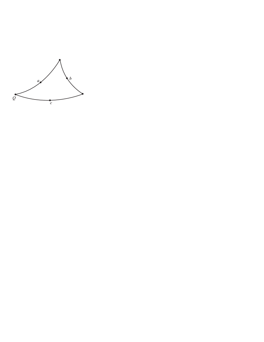
Figure 5: Fixed point $Q$ of the compound reflection $s_{c}s_{b}s_{a}$.

From (5.7), (5.9) it follows that

$$\ (2\pi\hbar)^{n}\!\int_{\mathcal{M}}\!\mbox{\rm Tr}\left(\Delta_{(a,\xi)}\,\Delta_{(b,\eta)}\,\Delta_{(c,\zeta)}\right)\phi(c)\,dm(c)=\int_{\mathcal{M}}\!T_{a,b,c}^{\xi,\eta,\zeta}(q)\mathcal{J}_{a,b,c}(q)^{-1}\phi(c)\left|\frac{\mathcal{D}m(c)}{\mathcal{D}(q)}\right|\,dm(q)\,,$$

and so, one has the following formula for the distribution $K_{\star}$ in (2.8)

$$K_{\star}(x,y,z)=(2\pi\hbar)^{n}\,\mbox{\rm Tr}\left(\Delta_{(a,\xi)}\,\Delta_{(b,\eta)}\,\Delta_{(c,\zeta)}\right)=\sum_{Q}\frac{1}{\mathcal{J}_{a,b,c}(Q)}\ T_{a,b,c}^{\xi,\eta,\zeta}(Q)\,.$$ (5.12)

The summation is taken over all fixed points of (5.11).

If the triple $(a,b,c)$ is such that there is no solution of the fixed point problem (5.11), then the value of the trace (5.12) is just zero.

If the triple $(a,b,c)$ is such that there is a solution of the fixed point problem (5.11) which is not infinitesimally isolated (the Jacobian (5.10) is zero), then the value of the trace (5.12) is infinite. The precise description of what this ‘infinity’ actually is, is given by the integral (5.7) (where there are no singularities at all).

Note that the amplitude factor on the right hand side of formula (5.12) is derived from (5.3), (5.5) and the definition of the Jacobian $J_{a}$ at the beginning of Sect. 3. Thus we obtain the amplitude

$$\varphi(a,b,c)\stackrel{{\scriptstyle\mathrm{def}}}{{=}}\varphi_{a,b,c}(Q)=2^{n}\left[j_{a}(Q)j_{b}(s_{a}(Q)j_{c}(s_{b}s_{a}(Q))\cdot\big{|}\det d(s_{c}s_{b}s_{a})(Q)\big{|}\right]^{1/2}\,,$$ (5.13)

where $Q=Q(a,b,c)$ is the solution of (5.11).

The phase of the exponential factor in (5.12) can be represented in the following geometrical form.

Lemma 9.

$$S_{a,b,c}^{\xi,\eta,\zeta}(Q)=\int_{\Sigma(x,y,z)}\omega\,.$$ (5.14)

Here the symplectic form $\omega$ is determined by (1.3), the points $x,y,z\in T^{*}\!\mathcal{M}$ are given by (5.1) and $\Sigma(x,y,z)$ is a triangle in $T^{*}\!\mathcal{M}$ whose sides are $\sigma$-reflective curves with midpoints $x,y,z$.

Indeed, the symplectic area on the right hand side of (5.14), by Stokes theorem, can be represented as the sum of three integrals

$$\int_{\Sigma(x,y,z)}\omega=\int_{Q^{\prime}}^{Q}(\tilde{p}\,d\tilde{q}+A^{0})+\int_{Q^{\prime\prime}}^{Q^{\prime}}(\tilde{p}\,d\tilde{q}+A^{0})+\int_{Q}^{Q^{\prime\prime}}(\tilde{p}\,d\tilde{q}+A^{0})\,.$$ (5.15)

Here $Q^{\prime}=s_{a}(Q)\,,Q^{\prime\prime}=s_{b}s_{a}(Q)\,,$ each integral (5.15) is taken along the geodesics through the midpoints $a,b,c$ respectively, and $\tilde{p}\in T^{*}\!\mathcal{M}$ denotes the value of the momentum on the $\sigma$-reflective curves over these geodesics. The magnetic potential $A^{0}$ is a primitive of the Faraday form $dA^{0}=F$. Using (3.23) we conclude that the three integrals of $A^{0}$ in (5.15) correspond to three summands with the functions $\Phi_{a},\Phi_{b},\Phi_{c}$ in (5.4), and the three other integrals of $\tilde{p}\,d\tilde{q}$ contribute to the terms containing the momenta $\xi,\eta,\zeta$. For example, in the first integral of (5.15) one has

$$\int_{Q^{\prime}}^{Q}\tilde{p}\,d\tilde{q}=\int_{Q^{\prime}}^{Q}\big{(}dV_{a}(\tilde{q})^{*}\xi-b_{a}(\tilde{q})\big{)}\,d\tilde{q}=\int_{Q^{\prime}}^{Q}d\big{(}\xi V_{a}(\tilde{q})\big{)}=\xi V_{a}(Q)-\xi V_{a}(Q^{\prime})=2\xi V_{a}(Q)\,.$$

In the above formula $b_{a}\equiv A^{0}-\frac{1}{2}d\Phi_{a}$ is used to make the curve $\{(\tilde{q},\tilde{p})\}$ to be $\sigma$-reflective with respect to the midpoint $x=(a,\xi)$.

Thus from (2.7), (2.8) and the formulas (5.12), (5.13), (5.14) we obtain the following result

$$(f\star g)(x)=\frac{1}{(\pi\hbar)^{2n}}\int\!\!\int_{C(\underline{x})}\sum\exp\Big{\{}\frac{i}{\hbar}\int_{\Sigma(x,y,z)}\omega\Big{\}}\,\frac{\varphi(\underline{x},\underline{y},\underline{z})}{\mathcal{J}(\underline{x},\underline{y},\underline{z})}f(y)g(z)\,dy\,dz\,.$$ (5.16)

In this formula

• all objects are independent of the choice of the measure on the manifold $\mathcal{M}$ and are determined by an affine structure $\underline{\Gamma}$ and a closed $2$-form $F$ on $\mathcal{M}$;

• points $x,y,z$ belong to the phase space $T^{*}\!\mathcal{M}$, and points $\underline{x},\underline{y},\underline{z}$ are their projections onto $\mathcal{M}$;

• the positive function $\varphi\in C^{\infty}(\mathcal{M}\times\mathcal{M}\times\mathcal{M})$ is given by (5.13);

• the Jacobian $\mathcal{J}(\underline{x},\underline{y},\underline{z})=\big{|}\det\big{(}I-d(s_{\underline{z}}s_{\underline{y}}s_{\underline{x}})(Q)\big{)}\big{|}$ is determined by the differential of the composition $s_{\underline{z}}s_{\underline{y}}s_{\underline{x}}$ of three $\underline{\Gamma}$-geodesic reflections in $\mathcal{M}$ with respect to midpoints $\underline{z},\underline{y},\underline{x}$, and where $Q$ is the fixed point of this composition;

• the magnetic form $\omega$ (1.3) is integrated in (5.16) over surfaces (or membranes) which are ‘triangles’ $\Sigma(x,y,z)$ in $T^{*}\!\mathcal{M}$ whose sides are $\sigma$-reflective curves with midpoints $x,y,z$. The projection of $\Sigma(x,y,z)$ onto $\mathcal{M}$ are geodesic triangles $\underline{\Sigma}(\underline{x},\underline{y},\underline{z})$ with midpoints $\underline{x},\underline{y},\underline{z}$;

• the domain of integration in (5.16) is a cotangent ‘cylinder’ $C(\underline{x})=T^{*}(\mathcal{M}\times_{\underline{x}}\mathcal{M})$ over the subset $\mathcal{M}\times_{\underline{x}}\mathcal{M}$ consisting of all those pairs of points $\underline{y},\underline{z}\in\mathcal{M}\times\mathcal{M}$ for which the triangle $\underline{\Sigma}(\underline{x},\underline{y},\underline{z})$ exists. The sum $\sum$ is taken over all such triangles.

Theorem 1.

The associative product of functions over the phase space $T^{*}\!\mathcal{M}$, which corresponds via (2.3) to the magneto-geodesic quantization, is determined by the formula (5.16). This formula acts directly on the subalgebra $\mathcal{F}(T^{*}\!\mathcal{M})$ of functions whose momentum Fourier image belongs to $\mathcal{D}(T\mathcal{M})$, and is extended to the algebra $\mathcal{F}_{\star}$ (and to its subalgebra $\mathcal{P}$) by the procedure (2.11).

The subset $\mathcal{M}\times_{\underline{x}}\mathcal{M}$ can be called the domain of influence of the point $\underline{x}\in\mathcal{M}$. Inside $\mathcal{M}\times_{\underline{x}}\mathcal{M}$ the Jacobian​ $\mathcal{J}$ is not zero. In general the domain of influence $\mathcal{M}\times_{\underline{x}}\mathcal{M}$ does not coincide with the whole $\mathcal{M}\times\mathcal{M}$. So, if the function $f\otimes g$ is localized outside of $C(\underline{x})$, then the integral (5.16) vanishes in a neighborhood of the fiber $T^{*}_{\underline{x}}\mathcal{M}$.

As an example consider the Lobachevski plane, $\mathcal{M}=H^{2}$, given by the hyperboloid in three dimensional Euclidean space : $H^{2}\equiv\{q\in{\mathbb{R}}^{3}|\,q_{1}^{2}+q_{2}^{2}-q_{3}^{2}=-1\}$. The Riemannian structure on $H^{2}$ is induced from the Euclidean structure on ${\mathbb{R}}^{3}$; the connection $\underline{\nabla}$ on $H^{2}$ is the usual Levi-Civita connection. In this case it is known (cf. [68, 69] ) that the geodesic triangle with midpoints $\underline{x}\,\underline{y}\,\underline{z}$ exists iff

$$-1<\det|\underline{x}\,\underline{y}\,\underline{z}|<1$$ (5.17)

(here $\underline{x}\,\underline{y}\,\underline{z}$ are considered to be 3-vectors, and $|\underline{x}\,\underline{y}\,\underline{z}|$ denotes the $3\times 3$ matrix of their components). Under the condition (5.17) such a triangle is unique. If one fixes $\underline{y}\,,\underline{z}$ then the subset $H_{\underline{y}\,\underline{z}}$ of points $\underline{x}\in H^{2}$ obeying (5.17) looks like a tubular neighborhood of the geodesic passing through $b$ and $c$. Certainly $H_{\underline{y}\,\underline{z}}$ is a proper subset in $H^{2}$, that is $H_{\underline{y}\,\underline{z}}\neq H^{2}$ if $\underline{y}\neq\underline{z}$. Thus, if $\underline{x}\notin H_{\underline{y}\,\underline{z}}$ then $(\underline{y}\,,\underline{z})\notin H^{2}\times_{\underline{x}}H^{2}$. Therefore, the domain of influence $H^{2}\times_{\underline{x}}H^{2}$ is a proper subset in $H^{2}\times H^{2}$.

We see that the quantum product (5.16) determines the distribution

$$K_{\star}(f\otimes g\otimes l)=\langle f\star g,l\rangle\,,$$ (5.18)

whose support, in general, does not coincide with the whole $T^{*}\!\mathcal{M}\times T^{*}\!\mathcal{M}\times T^{*}\!\mathcal{M}$. The topological boundary of this support can be considered as a quantum front

$${\mathrm{front}}\,(\star)\stackrel{{\scriptstyle\mathrm{def}}}{{=}}\partial({\mathrm{supp}}\,K_{\star})\,.$$ (5.19)

From one side of this boundary the distribution $K_{\star}$ is identically zero. We call this phenomenon a front-effect.

Something close to this was mentioned in the interesting note [69] following ideas of geometric quantization, but no actual construction of any associative product was produced there.

The phase space of the type $T^{*}\!\mathcal{M}$, which we investigate in this paper, and in particular the space $T^{*}H^{2}$ seems to be the first instance where the front-effect for the $\star$ product is mathematically identified.

The kernel $K_{\star}$ can be considered as a product of two $\delta$-functions

$$K_{\star}(x,y,z)=\big{(}\delta_{y}\star\delta_{z}\big{)}(x)\,.$$

The set supp$(\delta_{y}\star\delta_{z})$ is the cylinder $T^{*}\mathcal{M}_{\underline{y}\underline{z}}$ over the domain $\mathcal{M}_{\underline{y}\underline{z}}\subset\mathcal{M}\times\mathcal{M}$ (consisting of those $\underline{x}$ for which the geodesic triangle $\underline{\Sigma}(\underline{x},\underline{y},\underline{z})$ exists). Outside of this cylinder the distribution $\delta_{y}\star\delta_{z}$ is identically zero. The boundary of $T^{*}\mathcal{M}_{\underline{y}\underline{z}}$ is a front of the ‘wave’ $\delta_{y}\star\delta_{z}$ which travels in the phase space $T^{*}\!\mathcal{M}$ when the points $\underline{y}$ and $\underline{z}$ move away from each other.

Note that it is not possible to detect the front-effect in classical mechanics or even in the formal deformation approach where instead of exact associative product like (5.16) one uses a formal asymptotic power series in $\hbar$.

Also note that in the approach based on ideas of pseudodifferential operator theory [26, 28, 29, 34], where the $\star$-product is considered only on symbols whose $p$-Fourier transform is localized near zero, one can introduce under the integral (5.16) a cutoff function. This function is identically 1 for $x,y,z$ close enough to each other, but becomes $0$ if $x,y,z$ move away from each other. In this way one can eliminate all the difficulties related to the possible existence of conjugate points on geodesics or the non-existence of triangles. The formula (5.16), with the cutoff function, works for arbitrary affine manifolds $\mathcal{M}$; no front effect exists in this approach and no summation over multiple triangles is needed. Of course, this ‘cutoff method,’ in general, destroys the associativity of the $\star$-product. But with this approach one can keep associativity in the algebra $\mathcal{P}$ of symbols polynomial in momenta. Thus, we conclude that formula (5.16) works in the algebra $\mathcal{P}$ over an arbitrary manifold $\mathcal{M}$.

Looking forward to Sect. 6 we note that the coefficients of the asymptotic expansion (1.6), (6.1) of the $\star$ product are insensitive to the cutoff function, since they are derived from the diagonal of the exact product (5.16). Thus, the $\hbar\to 0$ asymptotic expansion of the product (5.16) works over an arbitrary manifold $\mathcal{M}$.

We stress that the core result of Theorem 1 is the explicit formula for an associative quantum product over the phase space $T^{*}{\cal M}$. This formula is exact, not a deformation one, and even not a semiclassical one. Under the semiclassical approach the leading term of the asymptotics of the product kernel $K_{\star}$ is known over general phase spaces [70]. The membrane formula like (5.14) for the phase of $K_{\star}$ was first suggested in [71] as a formula for the ‘action’ on the graph of groupoid multiplication, and it was proved in [70], in the general symplectic case, that indeed (5.14) is the correct solution of the Cauchy problem for the phase function. In the Euclidean case, membrane formulas of a similar type were discovered by M. Berry [72] for the asymptotics of the Wigner function (see also [73] for solutions of the Cauchy problem). The magnetic version of these formulas was first obtained and investigated in detail in [4, 5], the case of symmetric spaces was studied in [74], and for general manifolds, see in [75, 76].

6 Magneto-geodesic connection and $\hbar$-expansion of the quantum product

In this section we investigate the asymptotic properties of the product $f\star g$ in the classical approximation as $\hbar\rightarrow 0$ and express the results in terms of magneto-geodesic covariant derivatives over phase space $T^{*}\!\mathcal{M}$. It is assumed that the functions $f,g$ are $\hbar$-independent.

The integral (5.16) determing the quantum product contains a rapidly oscillating exponential factor and a smooth (non-oscillating) amplitude. The exponent phase has a stationary point at $y=x,\,z=x$, which is isolated and non-degenerate. Therefore one can apply the standard stationary phase method [77] to derive the asymptotic expansion of the integral (5.16) as $\hbar\rightarrow 0$. The structure of this expansion is

$$(f\star g)(x)=\sum_{k\geq 0}\frac{1}{k!}\left({\frac{-i\hbar}{2}}\right)^{k}G_{k}(f\otimes g)(x)\,.$$ (6.1)

Here $G_{k}$ are differential operators of order $2k$ acting on the function $f(y)\,g(z)$ and then restricted to the diagonal (the stationary point) $y=x,\,z=x\,$.

Since we know that the unity function $1$ is the unit element for the $\star$-product, then

$$\begin{array}[]{l}G_{0}(f\otimes 1)=f\,,\phantom{\Big{(}}\\ G_{k}(f\otimes 1)=G_{k}(1\otimes f)=0\,,\qquad k\geq 1\,.\end{array}$$ (6.2)

From (6.2) it follows, for instance, that

$$\quad G_{0}(f\otimes g)=fg\,,\qquad G_{1}(f\otimes g)=\langle df,\Psi\,dg\rangle$$

where $\Psi$ is a 2-tensor. From the property (2.9) and the involution property $\overline{f\star g}=\overline{g}\star\overline{f}$ we see that $\Psi$ must be skew-symmetric and real. In addition, the associativity of the $\star$-product implies the Jacobi identity for $\Psi$. Thus $\Psi$ is a Poisson tensor on $T^{*}\!\mathcal{M}$. It is easy to check that $\Psi=\Omega^{-1}$, where $\Omega$ is the matrix of the symplectic form $\omega$ in the exponent of (5.16).

Thus the expansion of (6.1) takes the form

$$f\star g=fg-\frac{i\hbar}{2}\{f,g\}-\frac{\hbar^{2}}{8}\,G_{2}(f\otimes g)\big{|}_{diag}+O(\hbar^{3})$$ (6.3)

with the Poisson bracket $\{f,g\}\equiv\langle df,\Psi dg\rangle\,.$

In the general theory of deformation quantization [42, 47, 48, 50] it was observed that the operator $G_{2}$ in expansions of star-products like (6.3) has to be related to a certain phase space connection $\nabla$, and moreover, $G_{2}$ can be written in the form

$$G_{2}=(\nabla^{\prime}\Psi\nabla^{\prime\prime})^{2}+\nabla^{\prime}\mathcal{B}\nabla^{\prime\prime}\,.$$ (6.4)

Here $\mathcal{B}$ is a certain 2-tensor, and the primes mark the argument (first or second) of the function $f\otimes g$ to which the covariant derivative $\nabla$ is applied.

For our specific (and exact) quantum product $\star$ over $T^{*}\!\mathcal{M}$ the generic form $(\ref{VI.4})$ can be verified and explicit formulas for $\nabla$ and $\mathcal{B}$ can be found directly from the asymptotic expansion of the integral (5.16).

But we also could match the quantization with a phase space connection in another way. The quantization is given by the quantizer $\Delta_{x}$, which in turn defines a family of symplectic transformations $\sigma_{x}$ via (4.13). The transformations $\sigma_{x}$ acting on $T^{*}\!\mathcal{M}$ are the phase space analogs of the geodesic reflections $s_{q}$ acting on $\mathcal{M}$. These later reflections are generated by the connection $\underline{\nabla}$ over $\mathcal{M}$. The Christoffel symbols of this connection are determined via $s_{q}$ as follows

$$\ \underline{\Gamma}(q)=-\frac{1}{2}\,D^{2}s_{q}(q^{\prime}){\big{|}}_{q^{\prime}=q}\,,$$

where $D$ denotes derivatives with respect to argument $q^{\prime}\in\mathcal{M}$. We can just mimic this formula to define a connection over $T^{*}\!\mathcal{M}$

$${\Gamma}(x)=-\frac{1}{2}\,D^{2}\sigma_{x}(x^{\prime}){\big{|}}_{x^{\prime}=x}\,,$$ (6.5)

where $D$ denotes derivatives by the argument $x^{\prime}\in T^{*}\!\mathcal{M}$. This formula indeed generates a connection for any family of reflections, and such a connection is automatically symplectic if these reflections are symplectic [70]. In our magneto-geodesic situation we have all these properties of the family $\{\sigma_{x}\}$ (Corollary 3; for the Euclidean case $\mathcal{M}=R^{n}$, see more details in [5]).

Note that the restriction of $\sigma_{x}$ to the configuration space $\mathcal{M}$ coincides with $s_{q}$ (see (4.13)), and so, the set of Christoffel symbols $\Gamma$ (6.5) contains the Christoffel symbols $\underline{\Gamma}$ inside itself. Thus $\Gamma$ is an extension of $\underline{\Gamma}$ from the configuration space to the phase space.

Explicit calculation of the second derivatives in (6.5) using (4.13), yields

$$\Gamma_{qq}^{q}={\underline{\Gamma}}(q)\,,\qquad\Gamma_{qp}^{p}=\Gamma_{pq}^{p}=-\underline{\Gamma}(\,q)\,,\qquad\Gamma_{qq}^{p}=p\,B(q)+C(q)\,, a$$ (6.5)

where

$$B^{m}_{jkl}\stackrel{{\scriptstyle\mathrm{def}}}{{=}}\frac{1}{3}\,\underset{jkl}{\mathfrak{S}}\left(2\,\underline{\Gamma}_{\,js}^{m}\,\underline{\Gamma}_{\,kl}^{s}-\partial_{j}\,\underline{\Gamma}_{\,kl}^{m}\right)\,,\qquad C_{jkl}\stackrel{{\scriptstyle\mathrm{def}}}{{=}}\frac{1}{3}\,(\underline{\nabla}_{\,k}\,F_{jl}+\underline{\nabla}_{\,l}\,F_{jk})\,, b$$ (6.5)

and the notation ${\mathfrak{S}}$ denotes cyclic summation. All other components of $\Gamma$ vanish identically: $\Gamma_{pq}^{q}=\Gamma_{qp}^{q}=\Gamma_{pp}^{q}=\Gamma_{pp}^{p}=0$ .

Let $\nabla$ be the covariant derivative over $T^{*}\!\mathcal{M}$ defined by Christoffel symbols (6.5$a$). We call it the magneto-geodesic connection. We stress again that this connection is symplectic with respect to the ‘magnetic’ symplectic structure $\omega$ (1.3), i.e.,

$$\nabla\omega=0.$$

We see that such a $\nabla$ is certainly related to the quantizer and so also to the $\star$-product (5.16). We claim that this is actually the same connection which appears in (6.4) under the $\hbar$-expansion of integral (5.16).

Now we demonstrate how to prove this claim. Let us fix $x=(a,\xi)\in T^{*}\!\mathcal{M}$. Formula (5.4) implies that there is just one stationary point of the phase function $S=S^{\xi,\eta,\zeta}_{a,b,c}$ with respect to variables $y=(b,\eta)$ and $z=(c,\zeta)$, namely, this is the point $y=x\,,z=x$. Near this point only one summand in (5.16) contributes to the asymptotic expansion up to $O(\hbar^{\infty})$, namely, this is the summand corresponding to small triangles $\Sigma=\Sigma(x,y,z)$ near the point $x$. Consider $x$ as the origin of the normal coordinate system (with respect to the connection (6.5)). We employ normal coordinates for both variables $y,z$ in (5.16). With this adjustment the integral looks like

$$f\star g\sim\int_{{\mathbb{R}}^{2n}}\int_{{\mathbb{R}}^{2n}}\,e^{{\frac{i}{\hbar}}S(v^{\prime},v^{\prime\prime})}\,L(v^{\prime},v^{\prime\prime})\,f\big{(}\exp_{x}(v^{\prime})\big{)}\,g\big{(}\exp_{x}(v^{\prime\prime})\big{)}\,{\frac{dv^{\prime}\,dv^{\prime\prime}}{(\pi\hbar)^{2n}}}\,.$$ (6.6)

Here the integration space, ${\mathbb{R}}^{2n}\times{\mathbb{R}}^{2n}$, is just $T_{x}(T^{*}\!\mathcal{M})\times T_{x}(T^{*}\!\mathcal{M})$; $v^{\prime}\,v^{\prime\prime}$ are normal coordinates, and the phase function $S=\int_{\Sigma}\omega$, cf. (5.14). The amplitude function $L$ is given by (5.10), (5.13): namely, $L=(\varphi/\mathcal{J})\,l\otimes l$, where $l$ is the density of the Liouville measure on $T^{*}\!\mathcal{M}$ expressed in normal coordinates.

Lemma 10.

The following Taylor expansions hold

$$S=S_{2}+S_{4}+O^{6}\,,\quad L=1+L_{2}+O^{4}\,,\quad l=1+l_{2}+O^{4}$$ (6.7)

where $S_{2},L_{2},l_{2}$ are homogeneous polynomials of degree $2$, and $S_{4}$ is of degree $4$; the remainders $O^{4}\,,O^{6}$ are of degree $4$ and $6$ in normal coordinates near zero in ${\mathbb{R}}^{2n}\otimes{\mathbb{R}}^{2n}$. Formulas for the quadratic forms $S_{2}$ and $L_{2}$ are

$$S_{2}(v^{\prime},v^{\prime\prime})=2\,\langle\Omega v^{\prime\prime},v^{\prime}\rangle\,,\qquad L_{2}(v^{\prime},v^{\prime\prime})=-{\frac{1}{2}}\,\langle\underline{\mathcal{R}}(\underline{v}^{\prime}-\underline{v}^{\prime\prime}),\underline{v}^{\prime}-\underline{v}^{\prime\prime}\rangle+l_{2}(v^{\prime})+l_{2}(v^{\prime\prime})\,.$$ (6.8)

Here $\Omega$ is the $2n\times 2n$ matrix of the symplectic form, $\Omega=\big{[}\begin{array}[]{cc}F&I\\ -I&0\end{array}\big{]}$, $\underline{v}\in{\mathbb{R}}^{n}$ denotes the $q$-components of the vector $v\in{\mathbb{R}}^{2n}={\mathbb{R}}_{q}^{n}\times{\mathbb{R}}_{p}^{n}$, and $\underline{\mathcal{R}}$ is the symmetric part of the $n\times n$ Ricci tensor on $\mathcal{M}$

$$\underline{\mathcal{R}}_{\,ls}\stackrel{{\scriptstyle\mathrm{def}}}{{=}}{\frac{1}{2}}\,(\underline{R}^{\,k}_{\ lks}+\underline{R}^{\,k}_{\ skl})\,,$$ (6.9)

where $\underline{R}=[\,\underline{\nabla}\,,\underline{\nabla}\,]$ is the curvature tensor (skew symmetric in the last pair of indices).

Proof. The first formula in (6.8) is obvious. Indeed from (5.14) we claim that

$$S=\frac{1}{2}\,\Omega\,V^{\prime\prime}\,V^{\prime}+O^{4}\,,$$

where $V^{\prime},V^{\prime\prime}$ are the sides of the linearization of the triangle $\Sigma(x,y,z)$ at the point $x=(a,\xi)$. The sides $V^{\prime},V^{\prime\prime}$ are twice as long as the normal coordinates $v^{\prime},v^{\prime\prime}$ of the midpoints $y=(b,\eta),z=(c,\zeta)$ of this triangle. This is the reason for the factor of $2$ in the first formula of (6.8).

To prove the second formula in (6.8) we first deduce from (5.10) and (5.13) that

$$L_{2}(v^{\prime},v^{\prime\prime})=l_{2}(v^{\prime})+l_{2}(v^{\prime\prime})+\alpha_{2}(\underline{v}^{\prime},\underline{v}^{\prime\prime})+\beta_{2}(\underline{v}^{\prime},\underline{v}^{\prime\prime})\,.$$ (6.10)

Here $\alpha_{2}$ and $\beta_{2}$ are the second order Taylor terms about the point $a$ of the functions

$$\begin{array}[]{l}\alpha\stackrel{{\scriptstyle\mathrm{def}}}{{=}}2^{n}\big{|}\det d(s_{c}s_{b}s_{a})(Q)\big{|}^{1/2}\,\mathcal{J}^{-1}(Q)\,,\phantom{\Biggr{)}}\\ \beta\stackrel{{\scriptstyle\mathrm{def}}}{{=}}\big{[}j_{a}(Q)\,j_{b}(s_{a}(Q))\,j_{c}(s_{b}s_{a}(Q))\big{]}^{1/2}\end{array}$$ (6.11)

where $Q$ is the solution of the problem (5.11) in the neighborhood of the origin point $a$.

The Taylor expansion of $Q$, in normal coordinates, results from

$$Q=\underline{\exp}\,_{a}(\underline{v}^{\prime\prime}-\underline{v}^{\prime}+O^{2})\,.$$ (6.12)

The Jacobi matrix of the mapping $s_{c}s_{b}s_{a}$ reads

$$d(s_{c}s_{b}s_{a})\big{(}\underline{\exp}\,_{a}(\underline{v})\big{)}=-I+2\,(\underline{v}^{\prime\prime}-\underline{v}^{\prime}-\underline{v})\,\underline{\Gamma}+O^{2}\,.$$

From here and (6.12) it follows that

$$d(s_{c}s_{b}s_{a})=-I+O^{2}\,,$$

and so $\alpha=1+O^{4}$. This means that the second order Taylor term of the function $\alpha$ at the point $a$ is just zero: $\alpha_{2}=0$.

The Jacobians $j_{a},j_{b},j_{c}$ which compose the function $\beta$ in (6.11) are found in the beginning of Sect. 3. Here one has

$$j_{\,q}(\underline{\exp}\,_{q}(\underline{v}\,))=1-\frac{1}{3}\,\langle\underline{\mathcal{R}}\,\underline{v}\,,\underline{v}\rangle+O^{4}\,,$$

where $\underline{\mathcal{R}}$ is defined by (6.9). Therefore

$$\beta=1-\frac{1}{2}\,\langle\underline{\mathcal{R}}\,(\underline{v}^{\prime\prime}-\underline{v}^{\prime}),\underline{v}^{\prime\prime}-\underline{v}^{\prime}\rangle+O^{4}\,.$$

Combining this with (6.10) we conclude that the second formula in (6.8) holds. $\square$

Lemma 11.

The fourth degree contribution $S_{4}$ in expansion (6.7) satisfies the following estimate

$$\langle\partial^{\prime},\Psi\partial^{\prime\prime}\rangle S_{4}(v^{\prime},v^{\prime\prime})=O^{2}(\underline{v}^{\prime})+O^{2}(\underline{v}^{\prime\prime})\,.$$ (6.13)

Proof. The exponential map corresponding to Christoffel symbols (6.5$a$) has the Taylor expansion

$$\exp_{a,\xi}(v)=\begin{pmatrix}a+\underline{v}-\frac{1}{2}\,{\underline{\Gamma}}(a)\,{\underline{v}}\,{\underline{v}}+\frac{1}{6}\,B(a)\,\underline{v}\,\underline{v}\,\underline{v}+O(\underline{v}^{4})\\ \,\xi+\underline{\underline{v}}+\underline{\Gamma}(a)\,\,\underline{v}\,\underline{\underline{v}}-\frac{1}{2}\,\big{(}\xi\,B(a)+C(a)\big{)}\,\underline{v}\,\underline{v}\,+O({\underline{v}}^{3})+O({\underline{v}}^{2}\underline{\underline{v}})\,\phantom{\bigg{)}}\end{pmatrix}$$

where the matrices $B,\,C$ are defined in (6.5$b$), and by $\underline{\underline{v}}$ we indicate the $p$-component of the vector $v$.

From this formula and (5.4) we derive the following expression for the fourth degree component $S_{4}$ of the phase function:

$$\ S_{4}(v^{\prime},v^{\prime\prime})=2\,\langle\underline{\Gamma}\ \underline{v}^{\prime}\,\underline{\underline{v}}^{\prime\prime}\,,\,\underline{\Gamma}\ \underline{v}^{\prime}\,\underline{v}^{\prime\prime}\rangle-2\,\langle\underline{\Gamma}\ \underline{v}^{\prime\prime}\,\underline{\underline{v}}^{\prime\prime}\,,\,\underline{\Gamma}\ \underline{v}^{\prime}\,\underline{v}^{\prime\prime}\rangle\,\phantom{\Big{)}}\\ +O\big{(}\underline{\underline{v}}^{\prime}\,{\underline{v}^{\prime\prime}}^{\,3}\big{)}+O\big{(}\underline{\underline{v}}^{\prime\prime}\,{\underline{v}^{\prime\prime}}^{\,3}\big{)}+O\big{(}\underline{\underline{v}}^{\prime}\,{\underline{v}^{\prime}}^{\,2}\,\underline{v}^{\prime\prime}\big{)}+O\big{(}\underline{\underline{v}}^{\prime\prime}\,{\underline{v}^{\prime\prime}}^{\,2}\,\underline{v}^{\prime}\big{)}+O^{3}\big{(}\underline{v}^{\prime}\,,\underline{v}^{\prime\prime}\big{)}\,.$$ (6.14)

Here the remainders do not contribute to the second order derivatives in $\langle\partial^{\prime},\Psi\partial^{\prime\prime}\rangle\,S_{4}$ and so we do not need to know their explicit expression. The first two terms in (6.14) provide formula (6.13). $\square$

Now we make the rescaling $v={\sqrt{\hbar}}\,u$ in the integrand of (6.6) and use Lemma 10 to get

$$f\star g\sim\int\!\!\int e^{iS_{2}(u^{\prime},u^{\prime\prime})}\left[1+\hbar\,(iS_{4}+L_{2})+O(\hbar^{2})\right](u^{\prime},u^{\prime\prime})\,\\ \times\,f\big{(}\exp_{x}(\sqrt{\hbar}u^{\prime})\big{)}\,g\big{(}\exp_{x}(\sqrt{\hbar}u^{\prime\prime})\big{)}\,\frac{du^{\prime}\,du^{\prime\prime}}{\pi^{2n}}\,.\qquad\qquad$$ (6.15)

By expanding the exponential mappings in (6.15) we reduce the calculation of the asymptotics of $f\star g$ to the evaluation of simple integrals like

$$\frac{1}{\pi^{2n}}\int\!\!\int\mathcal{P}_{2m}(u^{\prime},u^{\prime\prime})\,\exp\big{\{}2i\langle\Omega\,u^{\prime},u^{\prime\prime}\rangle\big{\}}\,du^{\prime}\,du^{\prime\prime}\\ =\sum_{r=0}^{m}\frac{(-i)^{r}}{2^{r}\,r!}\sum_{\,1\,\leq\,l_{j}\,,\ s_{j}\,\leq\,2n}\Psi^{l_{1}\,s_{1}}\cdots\Psi^{l_{r}\,s_{r}}\big{(}\partial_{l_{1}}^{\prime}\dots\partial^{\prime}_{l_{r}}\,\partial^{\prime\prime}_{s_{1}}\dots\partial^{\prime\prime}_{s_{r}}\mathcal{P}_{2m}\big{)}(0,0)$$ (6.16)

with some polynomials, $\mathcal{P}_{2m}$, of degree $2m$, where $m=0,1,\dots$.

In order to know the $k^{th}$ term in expansion (6.1) one must take into account contributions of integrals like (6.16) for degrees $2m\leq 2k$. In this way from (6.15) we obtain the expansion (6.3) and the formula (6.4) for the operator $G_{2}$, where the tensor $\mathcal{B}$ is given by

$$\mathcal{B}^{sl}=2\,\Psi^{sm}\,\Psi^{rl}\,\partial_{m}^{\prime}\,\partial_{r}^{\prime\prime}L_{2}+\Psi^{sm}\,\Psi^{rl}\,\Psi^{jk}\,\partial_{m}^{\prime}\,\partial_{j}^{\prime}\,\partial_{r}^{\prime\prime}\,\partial_{k}^{\prime\prime}\,S_{4}\,.$$ (6.17)

The second formula in (6.8) implies that

$$\partial^{\prime}\,\partial^{\prime\prime}L_{2}=\begin{pmatrix}\underline{\mathcal{R}}&0\\ 0&0\end{pmatrix}\,,$$

where $\underline{\mathcal{R}}$ is given by (6.9). From (6.13) one concludes that the second term in (6.17) vanishes. Therefore

$$\mathcal{B}=2\,\Psi\cdot\begin{pmatrix}\underline{\mathcal{R}}&0\\ 0&0\end{pmatrix}\cdot\Psi\,.$$ (6.18)

Proposition 5.

The curvature tensor $R$ of the magneto-geodesic connection $\nabla$ on $T^{*}\!\mathcal{M}$ is given by

$$R_{q^{i}q^{j}q^{k}}^{q^{s}} =\underline{R}_{\,ijk}^{\,s}\,,$$

$$R_{p_{j}q^{i}q^{k}}^{p_{s}} =\underline{R}_{\,ski}^{\,j}\,,\qquad\quad R_{q^{i}p_{j}q^{k}}^{p_{s}}=-R_{q^{i}q^{k}p_{j}}^{p_{s}}=\frac{1}{3}\,\big{(}\underline{R}^{j}_{\,ski}+\underline{R}^{j}_{\,iks}\big{)}\,,\phantom{\Bigg{)}}$$

$$R_{q^{i}q^{j}q^{k}}^{p_{s}} =\frac{1}{3}\,\,\underset{i\,s}{\mathfrak{S}}\,p_{m}\Big{(}\underline{\nabla}_{\,s}\,\underline{R}_{\ ikj}^{\,m}+3\,\underline{\Gamma}_{\ sl}^{\,m}\,\underline{R}^{\,l}_{\ ijk}-\underline{\Gamma}_{\ jl}^{\,m}\,\underline{R}^{\,l}_{\ iks}+\underline{\Gamma}_{\ kl}^{\,m}\,\underline{R}^{\,l}_{\ ijs}\Big{)}+M_{sijk}\,,$$

where

$$M_{sijk}\stackrel{{\scriptstyle\mathrm{def}}}{{=}}\ \frac{1}{3}\,\Big{(}\underline{\nabla}_{\,i}\underline{\nabla}_{\,s}\,F_{\,jk}+2\,\underline{R}^{\,l}_{\ ijk}\,F_{\,ls}+\underset{ijk}{\mathfrak{S}}\,\underline{R}^{\,l}_{\ sij}\,F_{\,lk}\Big{)}\,,\quad{(magnetic\ curvature)}\,.$$

Here $\underline{R}=\underline{R}(q)$ and $F=F(q)$ are the curvature of the connection $\underline{\nabla}$ and the magnetic tensor on $\mathcal{M}$. All other components of the curvature $R$ vanish.

We first remark that the block $R^{p}_{qqq}$ of the curvature tensor $R$ is not itself a tensor. But the part $M$, which we call the magnetic curvature, is a tensor on $\mathcal{M}$. This part of the total curvature entangles the magnetic field $F$ with the curvature tensor $\underline{R}$ on $\mathcal{M}$. Also note that the only $p$-dependent part of the curvature is the $R^{p}_{qqq}$ block (where $p$ enters linearly); all other parts are strictly $q$-dependent.

For any symplectic connection, the Ricci tensor

$$\mathcal{R}_{\,ij}\stackrel{{\scriptstyle\mathrm{def}}}{{=}}R_{\,ikj}^{\,k}$$ (6.19)

is symmetric [78]. Thus for the magneto-geodesic connection on $T^{*}\mathcal{M}$ we have $\mathcal{R}_{\,ij}=\mathcal{R}_{\,ji}$.

Corollary 5.

The Ricci tensor for the magneto-geodesic connection on $T^{*}\mathcal{M}$ is given by

$$\mathcal{R}=\frac{2}{3}\begin{pmatrix}\underline{\mathcal{R}}\phantom{\Big{)}}&0\\ 0&0\end{pmatrix}\,,$$ (6.20)

where $\underline{\mathcal{R}}$ is the symmetric part of the Ricci tensor for the affine connection on $\mathcal{M}$.

Now one just has to compare this formula for the Ricci tensor with formula (6.18) for the tensor $\mathcal{B}$ in the $\hbar$-expansion of the $\star$-product (6.3), (6.4).

Altogether we have proved the following statement.

Theorem 2.

The magneto-geodesic product (5.16) over $T^{*}\!\mathcal{M}$ has the asymptotic expansion (6.3) with the second order term $G_{2}$ given by the formula (6.4). In this formula the connection $\nabla$ coincides with the magneto-geodesic connection (6.5), (6.5$a$) and the tensor $\mathcal{B}$ is

$$\mathcal{B}=3\,\Psi\mathcal{R}\Psi\,,$$ (6.21)

where $\mathcal{R}$ is the Ricci tensor of this connection.

The magneto-geodesic connection $\nabla$ on $T^{*}\!\mathcal{M}$ entangles, on the phase space level, the original affine connection $\underline{\nabla}$ and the magnetic field (Faraday tensor) $F$ on $\mathcal{M}$. In the case of zero magnetic field $F=0$ this connection was obtained in [28] via a version of the deformation quantization approach by using a different star-product which does not obey axioms (2.6).

The part of the Christoffel symbol in (6.5$a$) which describes the ‘interaction’ between the affine and magnetic structures on $\mathcal{M}$ is given by the tensor $C$. The tensor $C$ contains the symmetrized covariant derivative of the magnetic tensor $F$. We label this part of the connection as the magneto-geodesic coupling tensor. The usual covariant derivative tensor $\underline{\nabla}F$ we call the magnetic inhomogeneity.

Let us examine the symmetric and skew-symmetric properties of these two tensors. We represent this pair of tensors with the notation

$$F_{[jk]l}\stackrel{{\scriptstyle\mathrm{def}}}{{=}}\underline{\nabla}_{\,l}\,F_{jk}\,,\qquad F_{j\{kl\}}\stackrel{{\scriptstyle\mathrm{def}}}{{=}}C_{jkl}\,.$$

Proposition 6.

(a) The magnetic inhomogeneity tensor $F_{[jk]l}$ is skew-symmetric in the first pair of indices; the magneto-geodesic coupling tensor $F_{j\{kl\}}$ is symmetric in the last pair of indices. They are related to each other by the following duality formulas

$$F_{j\{kl\}}={\frac{1}{3}}\big{(}F_{[jk]l}+F_{[jl]k}\big{)}\,,\qquad F_{[jk]l}=F_{j\{kl\}}-F_{k\{jl\}}\,.$$

(b) Both of these tensors obey the cyclic property

$$\underset{jkl}{\mathfrak{S}}\,F_{j\{kl\}}=0\,,\qquad\underset{jkl}{\mathfrak{S}}\,F_{[jk]l}=0\,.$$ (6.22)

(c) The magneto-geodesic coupling tensor is related to the magnetic curvature tensor $M$ by

$$\underline{\nabla}_{j}F_{s\{ik\}}-\underline{\nabla}_{k}F_{s\{ij\}}=M_{isjk}\,.$$

(d) On Riemannian manifolds $\mathcal{M}$ (with the Levi-Civita connection $\underline{\nabla}$ defined by metric $g$) the current covector

$$j_{s}=\frac{2}{3}F_{s\{ik\}}\,g^{ik}$$

satisfies the continuity equation $g^{ls}\underline{\nabla}_{\ l}j_{s}=0$, and generates the exact 2-form $\varkappa\equiv dj$ with coefficients

$$\varkappa_{sm}=g^{ik}\big{(}3M_{iksm}+2F_{il}\,\underline{R}_{ksm}^{l}\big{)}\,.$$

The identity $d\varkappa=0$, or ${\mathfrak{S}}\,\nabla_{r}\varkappa_{sm}=0$, ties together the magnetic curvature $M$ and the Riemannian curvature $\underline{R}$ on $\mathcal{M}$.

The last statement in (6.22) is just the homogeneous Maxwell equation for the magnetic field (that ensures that there are no Dirac monopoles), and the first identity in (6.22) is the ‘dual’ to the Maxwell equation and incorporates the magneto-geodesic coupling tensor.

Note that within the class of tensors obeying the condition ${\mathfrak{S}}\,C_{jkl}=0$, formulas (6.5$a$), (6.5$b$) determine a unique connection on $T^{*}\!\mathcal{M}$ having the property that the symplectic form is covariantly constant, $\nabla\omega=0$.

In the Euclidean case $\mathcal{M}={\mathbb{R}}^{n}$ the magneto-geodesic connection $\nabla$ coincides with the magnetic connection found in [5]. In this case the curvature tensor $R$ of $\nabla$ (see Proposition 5) is reduced to the magnetic curvature which is just the second derivative matrix $M_{sijk}=\frac{1}{3}\,D^{2}_{si}F_{jk}$. Thus the curvature $R$ is constant iff the field $F$ is quadratic in Euclidean coordinates. In this way we obtained in [5] an example of a symmetric symplectic space which can be explicitly and exactly quantized.

It should be interesting to study the equation

$$\nabla R=0$$ (6.23)

for the general magnetic-geodesic connection. Under condition (6.23) one again has an example of a symmetric symplectic structure, now on $T^{*}\!\mathcal{M}$, which is explicitly and exactly (not formally and not asymptotically) quantized. It would be interesting to compare this construction of quantized symmetric spaces with [79, 80].

Acknowledgments. The first author is grateful to Russian Foundation for Basic Research for partial support (grant No. 05-01-00918-a). The research of T.A.O. is supported by a grant from Natural Sciences and Engineering Research Council of Canada. The authors thank the Winnipeg Institute of Theoretical Physics for its continuing support.

References

[1]
H. J. Groenewold.
On the principles of elementary quantum mechanics.
Physica, 12:405–460, 1946.
[2]
J. E. Moyal.
Quantum mechanics as a statistical theory.
Proc. Cambridge Philos. Soc., 45:99–124, 1949.
[3]
F. A. Berezin.
Quantization.
Math. USSR-Izv., 8:1109–1165, 1974.
[4]
M. V. Karasev and T. A. Osborn.
Symplectic areas, quantization, and dynamics in electromagnetic
fields.
J. Math. Phys., 43:756–788, 2002;
preprint version in arXiv: quant-ph/0002041.
[5]
M. V. Karasev and T. A. Osborn.
Quantum magnetic algebra and magnetic curvature.
J. Phys. A., 37:2345–2363, 2004;
preprint version in arXiv: quant-ph/0311053.
[6]
R. Peierls.
Zur theorie des diamagnetismus von leitungselectronen.
Zeit. f. Physik, 80:763–775, 1933.
[7]
J. Schwinger.
On gauge invariance and vacuum polarization.
Phys. Rev., 82:664–679, 1951.
[8]
R. L. Stratonovich.
A gauge invariant analog of the Wigner distribution.
Sov. Phys. D, 1:414–418, 1956.
[9]
S. Fujita.
Introduction to non-equilibrium statistical mechanics.
Saunders, Philadelphia, 1966.
[10]
I. Bialynicki-Birula.
Classical limit of quantum electrodynamics.
Acta Physica Austrica, Suppl. XVIII:111–151, 1977.
[11]
V. Guillemin and S. Sternberg.
Symplectic Techniques in Physics.
Cambridge University Press, Cambridge, 1984.
[12]
O. T. Serimaa, J. Javanainen and S. Varró.
Gauge-independent Wigner functions: General formulation.
Phys. Rev. A, 33:2913–2927, 1986.
[13]
V. V. Dodonov, V. I. Man’ko and D. L. Ossipov.
Gradient-invariant Weyl representation. An oscillator in an
inhomogeneous magnetic field.
In: M. A. Markov, editor, Theory of Nonstationary Quantum
Oscillators, volume 198 of Proceedings of the Lebedev Physics
Institute, Nova Scince Publishers, Inc., pages 1–58, 1992.
[14]
M. Müller.
Product rule for gauge invariant Weyl symbols and its application
to the semiclassical description of guiding centre motion.
J. Phys. A, 32:1035–1052, 1999.
[15]
M. Măntoiu and R. Purice.
The magnetic Weyl calculus.
J. Math. Phys., 45:1394–1417, 2004.
[16]
P. A. M. Dirac.
Lectures on Quantum Mechanics.
Yeshiva University, New York, 1964.
[17]
G. W. Mackey.
Mathematical Foundations of Quantum Mechanics.
W. A. Benjamin, New York, 1963.
[18]
A. Lichnerowicz.
Twisted products for cotangent bundles of classical groups.
Lett. Math. Phys., 2:133–143, 1977.
[19]
J. Underhill.
Quantization on a manifold with connection.
J. Math. Phys., 19:1932–1935, 1978.
[20]
G. G. Emch.
Quantum and classical mechanics on homogeneous Riemannian
manifolds.
J. Math. Phys., 23:1785–1791, 1982.
[21]
S. Gutt.
An explicit -product on the cotangent bundle of a Lie group.
Lett. Math. Phys., 7:249–258, 1983.
[22]
M. de Wilde and P. Lecomte.
Star-products on cotangent bundles.
Lett. Math. Phys., 7:235–241, 1983.
[23]
J. Winter.
Wigner transformation in curved space-time and the curvature
correction of the Vlasov equation for semiclassical systems.
Phys. Rev. D, 32:1871–1888, 1985.
[24]
S. A. Fulling.
Pseudodifferential operators, covariant quantization, the inescapable
Van Vleck-Morett determinant, and the R/6 controversy.
In: Particle Physics and Cosmology, pages 329–342, Singapore,
1998. World Scientific.
[25]
Liu Zh.-J. and Qian, M.
Gauge invariant quantization on Riemannian manifolds.
Transac. Amer. Math. Soc., 331:321–333, 1992.
[26]
N. P. Landsman.
Strict deformation quantization of a particle in external
gravitational and Yang-Mills fields.
J. Geom. Phys., 12:93–132, 1993.
[27]
A. Connes.
Noncommutative Geometry.
Academic Press, London, 1994.
[28]
M. Bordemann, N. Neumaier, S. Waldmann.
Homogeneous Fedosov star products on cotangent bundles I:
Weyl and standard ordering with differential operator representation.
Commun. Math. Phys., 198:363–396, 1998;
preprint version in arXiv: q-alg/9707030.
[29]
M. Bordemann, N. Neumaier, S. Waldmann.
Homogeneous Fedosov star products on cotangent bundles II: GNS
Representations, the WKB expansion, and applications.
J. Geom. Physics, 29:199–234, 1999;
preprint version in arXiv: q-alg/9711016.
[30]
M. J. Pflaum.
A deformation-theoretical approach to Weyl quantization on
Riemannian manifolds.
Lett. Math. Phys., 45:277–294, 1998.
[31]
J. F. Cariñena, J. Clemente-Gallardo, E. Follana, J. M. Gracia-Bondía, A.
Rivero and J. C. Varilly.
Connes’ tangent groupoid and strict quantization.
J. Geom. Phys., 32:79–96, 1999;
preprint version in arXiv: DG/9802102.
[32]
S. T. Ali, N. M. Atakishiyev, S. M. Chumakov and K. B. Wolf.
The Wigner function for general Lie groups and the wavelet
transformation.
Ann. Henri Poincaré, 1:685–714, 2000.
[33]
M. Bordemann, N. Neumaier, M. Pflaum, and S. Waldmann.
On representations of star product algebras over cotangent spaces on
Hermitian line bundles.
J. Funct. Anal., 199:1–47, 2003;
preprint version in arXiv: QA/9811055.
[34]
H. Widom.
A complete symbolic calculus for pseudodifferential operators.
Bull. Sci. Math., 104:19–63, 1980.
[35]
H. Weyl.
Gravitation und Elektrizität.
Sitzungsberichte Akad. der Wissenschaften, pages 465–480,
1918.
[36]
N Straumann.
Early history of gauge theories and weak interactions.
arXiv: hep-ph/9609230, 1996.
[37]
G. S. Agarwal and E. Wolf.
Calculus for functions of noncommuting operators and general
phase-space methods in quantum mechanics. I. Mapping theorems and
ordering functions on noncommuting operators.
Phys. Rev. D, 2:2161–2186, 1970.
[38]
M. V. Karasev and V. E. Nazaikinskii.
On quantization of rapidly oscillating symbols.
Math. USSR-Sb., 34:737–764, 1978.
[39]
J. J. Slawianowski.
Abelian groups and the Weyl approach to kinematics.
Rep. Math. Phys., 5:295–319, 1974.
[40]
J. Krüger and A. Poffyn.
Quantum mechanics in phase space.
Physica, A85:84–100, 1976.
[41]
R. F. O’Connell and E. P. Wigner.
Quantum mechanical distribution functions: Conditions for
uniqueness.
Phys. Lett., 83A:145–148, 1981.
[42]
F. Bayen, M. Flato, C. Fronsdal, A. Lichnerowicz, and D. Sternheimer.
Deformation theory and quantization.
Ann. Phys. (N.Y.), 111:61–151, 1978.
[43]
M. Flato and D. Sternheimer.
Deformations of Poisson brackets.
In: M. de Wilde J. Wolf, M. Cahen, editor, Harmonic Analysis and
Representations of Lie Groups, page xx, Dordrecht, 1980. D. Riedel.
[44]
C. Fronsdal.
Some ideas about quantization.
Rep. Math. Phys., 15:111–145, 1979.
[45]
M. V. Karasev and V. P. Maslov.
Asymptotic and geometric quantization.
Russian Math. Surveys, 39:133–205, 1984.
[46]
M. Rieffel.
Deformation quantization for actions of .
Memoirs Amer. Math. Soc., 106:1–93, 1993.
[47]
H. Omori, Y. Maeda and A. Yoskioka.
Weyl manifolds and deformation quantization.
Advances in Mathematics, 85:224–255, 1991.
[48]
B. V. Fedosov.
A simple geometrical construction of deformation quantization.
J. Differential Geometry, 40:213–238, 1994.
[49]
M. Kontsevich.
Deformation quantization of Poisson manifolds, I.
Lett. Math. Phys., 60:157–216, 2003.
arXiv: math, q-alg/9709040, 1997.
[50]
S. Gutt and J. Rawnsley.
Natural star products on symplectic manifolds and quantum moment
maps.
Lett. Math. Phys., 66:123–139, 2003.
arXiv: math. SG/0304498, 2003.
[51]
J. von Neumann.
Wahrscheinlichkeitstheoretischer Aufbau der Quantenmechanik.
Göttinger Nachrichten, pages 245–272, 1927.
[52]
E. P. Wigner.
On the quantum correction for thermodynamic equilibrium.
Phys. Rev., 40:749–759, 1932.
[53]
R. L. Stratonovich.
On distributions in representation space.
Sov. Phys. JETP, 4:891–898, 1957.
[54]
J. Dixmier.
Les Algbres d’Oprateurs dans l’Espace
Hilbertien.
Gauther-Villars, Paris, 1969.
[55]
J. C. Varilly and J. M. Garcia–Bondia.
The Moyal representation of spin.
Ann. Phys. (N.Y.), 190:107–148, 1989.
[56]
A. Grossmann.
Parity operator and quantization of -functions.
Commun. Math. Phys., 48:191–194, 1976.
[57]
A. Royer.
Wigner function as the expectation value of a parity operator.
Phys. Rev. A, 15:449–450, 1977.
[58]
A. Grossmann and P. Huguenin.
Group-theoretical aspects of the Wigner–Weyl isomorphism.
Helvetica Physica Acta, 51:252–261, 1978.
[59]
J-P Amiet and M B Cibils.
Description of quantum spin using functions on the sphere .
J. Phys. A, 24:1515–1535, 1991.
[60]
J. M. Gracia-Bondia.
Generalized Moyal quantization on homogenous symplectic spaces.
Contemporary Mathematics, 134:93–114, 1992.
[61]
M. A. Antonets.
The classical limit for Weyl quantization.
Lett. Math. Phys., 2:241–245, 1978.
[62]
J. M. Gracia-Bondia and J. Varilly.
Algebras of distributions suitable for phase-space quantum mechanics.
I.
J. Math. Phys., 29:869–879, 1988.
[63]
J. Varilly and J. M. Gracia-Bondia .
Algebras of distributions suitable for phase-space quantum mechanics.
II Topogies of the Moyal algebra.
J. Math. Phys., 29:880–887, 1988.
[64]
G. B. Folland.
Harmonic Analysis in Phase Space.
Princeton University Press, Princeton, 1989.
[65]
F. H. Molzahn, T. A. Osborn and S. A. Fulling.
Gauge invariant asymptotic expansion of Schrödinger propagators
on manifolds.
Ann. Phys. (N.Y), 204:64–113, 1990.
[66]
J. G. Valatin.
Singularities of electron kernel functions in an external
electromagnetic field.
Proc. Soc. A, 222:93–108, 1954.
[67]
V. A. Fock.
On the canonical transformation in classical and quantum mechanics.
Vestnik Leningrad State Univ., 16:67–71, 1959 (in Russian).
[68]
G. M. Tuynman.
Areas of spherical and hyperbolic triangles in terms of their
midpoints.
U. Lille I - Math. preprint, 1999.
[69]
P. de Rios and G. M. Tuynman.
On Weyl quantization from geometric quantization.
arXiv:math-ph/0201044.
[70]