Qubit entanglement in multimagnon states

Abstract

The qubit entanglement induced by quasiparticle excitations in the Heisenberg spin chain and its relationship to the Bethe Ansatz structure of the eigenmodes is studied. A phenomenon called entanglement quenching, which suppresses eigenstate entanglement, is described and shown to be mediated by Goldstone magnons. Scattering states are characterized by short-range entanglement, and never exhibit entanglement at the longest range. In contrast, bound states have complex long-range entanglement structures.

I Introduction

The importance of quantum entanglement as a technological resource for quantum computing ForcerHeyRossSmith and quantum communication BennettWiesner , as an experimental requirement for Bell’s inequality violations OuMandel and other foundational tests of quantum mechanics, and as a central subject in the mathematical analysis of highly correlated states Keyl is now widely recognized. A fundamental theoretical problem is to understand the complex entanglement structure naturally present in systems as diverse as the Rindler vacuum PeresTerno , the photons produced through spontaneous parametric downconversion LawEberly , and the exchange-coupled spins of a magnet ArnesenBoseVedral . Much of the work on this problem to date has focused on ground state entanglement and its relation to quantum phase transitions QPT refs , or on thermal state entanglement and its modulation by magnetic fields ArnesenBoseVedral , thermal entanglement refs . In contrast, little is known about entanglement in excited states, or how this entanglement is related to quasiparticle interactions. The purpose of this paper is to address these latter issues by examining entanglement in a model system of interacting qubits, the Heisenberg spin chain.

The Heisenberg spin chain (HSC) is a one-dimensional lattice of spin-$1/2$ particles, with nearest-neighbor spins coupled by the exchange interaction. The HSC Hamiltonian is

$$H_{HSC}=J\sum^{N}_{i=1}{\mathbf{S}}_{i}\boldsymbol{\cdot}{\mathbf{S}}_{i+1},$$ (1)

where ${\mathbf{S}}_{i}=(S_{i}^{x},S_{i}^{y},S_{i}^{z})$ is the spin operator associated with the spin at the $i$th site of the lattice; its Cartesian components obey the usual angular momentum algebra. Periodic boundary conditions are assumed, so that ${\mathbf{S}}_{N+1}={\mathbf{S}}_{1}$. $J$ is the exchange coupling constant. States in the $2^{N}$-dimensional Hilbert space ${\mathcal{H}}$ of the model can be expanded in the “standard” basis of states of the form $|i,j,\ldots,k\rangle$, where the listed spins $i,j,\ldots,k$ are aligned in the $+z$-direction (‘up’) and the remaining spins are antiparallel (‘down’). $|\emptyset\rangle$ denotes the state with all spins down. The HSC and its anisotropic relatives have been the subject of considerable previous research in quantum information theory ArnesenBoseVedral ,QPT refs ,thermal entanglement refs .

The HSC model was originally solved by a method now termed the Bethe Ansatz (BA) Bethe . In the physical interpretation of this solution eigenstates are comprised of interacting quasiparticle excitations called magnons; the $a$th magnon is characterized by a pseudomomentum $k_{a}$, and there is a phase $\phi_{ab}$ between magnons $a$ and $b$. We would like to understand how the entanglement between the spins of the HSC, viewed as qubits, depends on the pseudomomenta and phases of the magnons. Unfortunately, as we will see, there is in general no simple relationship connecting qubit entanglement to these parameters. Nevertheless, the Bethe Ansatz formalism provides information that is not available from a direct numerical diagonalization of the Hamiltonian (although the BA equations themselves often must be solved numerically), and this information has much to tell us about the structure of qubit entanglement in the spin chain. Because the BA formalism is essential to the discussion, it is reviewed very briefly in the following section.

The entanglement between two spins will be quantified by calculating their concurrence concurrence , a measure of the inseparability of two-qubit pure or mixed states commonly used in quantum information theory. Other metrics, such as the entanglement of formation, can be calculated directly from the concurrence. Because the HSC Hamiltonian $H_{HSC}$ commutes with the total $z$-spin operator $S^{z}=\sum_{i=1}^{N}S_{i}^{z}$, the reduced density matrix (RDM) for any two spins in the states of interest always takes the form

$$\rho=\left(\begin{array}[]{cccc}\alpha&0&0&0\\ 0&\beta&\gamma&0\\ 0&\gamma^{*}&\delta&0\\ 0&0&0&\epsilon\end{array}\right).$$ (2)

For such a density matrix, the concurrence is

$$C=2\max\left(0,|\gamma|-\sqrt{\alpha\epsilon}\right).$$ (3)

Concurrence ranges from zero, for a separable state, to one, for a maximally entangled state. Because the states of the HSC which will be examined are translationally invariant, the concurrence depends only on the separation between the two spins. The concurrence between nearest-neighbor spins will be denoted $C_{1}$, between next-nearest-neighbor spins $C_{2}$, etc.

II Bethe Ansatz solution of the HSC

The Bethe Ansatz consists of the hypothesis that the coefficients of the expansions of the eigenstates of the HSC Hamiltonian (Eq. 1) with respect to the standard basis have the form of a permutation-invariant sum of $n!$ exponential terms, where $n$ is the number of spins inverted with respect to the reference state $|\emptyset\rangle$ Bethe . For example, the two-magnon eigenstates are assumed to have the form

$$|\psi(k_{1},k_{2},\phi_{12})\rangle=\nu(k_{1},k_{2},\phi_{12})\sum_{m_{1}<m_{2}}$$

$$\left(e^{ik_{1}m_{1}+ik_{2}m_{2}+i\phi_{12}/2}+e^{ik_{2}m_{1}+ik_{1}m_{2}-i\phi_{12}/2}\right)|m_{1},m_{2}\rangle,$$

where $\nu$ is a normalization constant. Substituting this state into the Schrödinger eigenvalue equation with the HSC Hamiltonian yields the constraints (the Bethe Ansatz equations, or BAE) which $k_{1}$, $k_{2}$, and $\phi_{12}$ must satisfy for the hypothesis to be correct:

$$2\cot\left(\frac{\phi_{12}}{2}\right) = \cot\left(\frac{k_{1}}{2}\right)-\cot\left(\frac{k_{2}}{2}\right),$$ (5)

$$Nk_{1}-\phi_{12} = 2\pi\lambda_{1},$$

$$Nk_{2}+\phi_{12} = 2\pi\lambda_{2}.$$

Note that under the interchange $k_{1}\leftrightarrow k_{2}$, $\phi_{12}$ changes sign, so that the wavefunction coefficients in Eq. II are permutation-invariant, as desired. $\lambda_{1}$ and $\lambda_{2}$ are integral quantum numbers between $0$ and $N-1$ whose allowed values are prescribed by an arcane set of rules Bethe . $k_{1}$ and $k_{2}$ are interpreted as the pseudomomenta of two magnons, and $\phi_{12}$ is a phase (the Bethe phase) between them.

The BA leads to a natural classification of two-magnon states as either scattering states or bound states. In scattering states each magnon has a real pseudomomentum between $0$ and $2\pi$, and the Bethe phase is real and between $0$ and $\pi$ if one chooses $k_{1}\leq k_{2}$. For such states the state vector (Eq. II) can be written in the form

$$|\psi(k_{1},k_{2},\phi_{12})\rangle=2\nu(k,\phi_{12})\sum_{m_{1}<m_{2}}$$

$$e^{iK(m_{1}+m_{2})/2}\cos{\scriptstyle{\frac{1}{2}}}\left(k(m_{2}-m_{1})+\phi_{12}\right)|m_{1},m_{2}\rangle,$$

where $k\equiv k_{2}-k_{1}$ is the relative pseudomomentum, $K\equiv k_{2}+k_{1}$ is the total pseudomomentum, and the normalization constant $\nu(k,\phi_{12})$ is

$$\nu^{-2}(k,\phi_{12})=N(N-1)+$$ (7)

$$\frac{N\cos(k-\phi_{12})-(N-1)\cos\phi_{12}-\cos(kN-\phi_{12})}{1-\cos(k)}.$$

This expression remains correct in the limit $k\rightarrow 0$. Even when the BAE are not satisfied, states of the above form (Eq. II) are properly normalized physical states (but not HSC eigenstates).

In bound states the magnons have complex conjugate pseudomomenta: $k_{1,2}=u\pm iv$. The imaginary component $v$ causes the probability distribution for the separation of the two inverted spins to be maximal when the spins are adjacent, and to decay exponentially as the separation between them increases. Due to this exponentially tight binding of the inverted spins, bound states exhibit entanglement behavior quite different from that of the scattering states, which (as will be shown) is controlled entirely by the binding parameter $v$. The bound states are of two types, both of which can usefully be put into forms independent of the Bethe phase. The $\cosh$-type bound (CB) states can be written as

$$|\psi_{C}(u,v)\rangle = \nu_{C}(v)\sum_{m_{1}<m_{2}}e^{iu(m_{1}+m_{2})}$$

$$\cosh\left[v\right(\frac{N}{2}-(m_{2}-m_{1})\left)\right]|m_{1},m_{2}\rangle,$$

where

$$\nu_{C}(v)=\left[\frac{4\sinh v}{N\left[\sinh\left((N-1)v\right)+(N-1)\sinh v\right]}\right]^{\frac{1}{2}},$$ (9)

while the $\sinh$-type bound (SB) states can be written as

$$|\psi_{S}(u,v)\rangle = \nu_{S}(v)\sum_{m_{1}<m_{2}}e^{iu(m_{1}+m_{2})}$$

$$\sinh\left[v\right(\frac{N}{2}-(m_{2}-m_{1})\left)\right]|m_{1},m_{2}\rangle,$$

where

$$\nu_{S}(v)=\left[\frac{4\sinh v}{N\left[\sinh\left((N-1)v\right)-(N-1)\sinh v\right]}\right]^{\frac{1}{2}}.$$ (11)

More generally, when there are $n$ magnons, the $n$ pseudomomenta and $n(n-1)/2$ phases satisfy a set of $n$ linear and $n(n-1)/2$ transcendental coupled BA equations. Multimagnon states can consist of all scattering magnons with real pseudomomenta, but more exotic states also appear. These include “wavecomplexes” (to use Bethe’s terminology Bethe ), which are solitons in which a group of magnons are all mutually bound, and mixtures of one or more wavecomplexes with scattering magnons. Note that instead of choosing as the reference state $|\emptyset\rangle$, the state with all spins down, one could equally well have chosen the state with all spins up, and statements which hold for $n$-magnon states can therefore be translated into equivalent statements for $(N-n)$-magnon states.

III Entanglement quenching

III.1 Two-magnon entanglement quenching

The zero-magnon eigenstate of the HSC is the reference state $|\emptyset\rangle$; it is of course a pure product state. The excitation of a single magnon changes this dramatically. The one-magnon eigenstates have the expected BA form

$$|\psi(k_{1})\rangle=\frac{1}{\sqrt{N}}\sum_{m=1}^{N}e^{ik_{1}m}|m\rangle,$$ (12)

where $k_{1}=2\pi\lambda_{1}/N$ and $\lambda_{1}$ is a quantum number that takes integral values between $0$ and $N-1$. Remarkably, the spins of the HSC are now equientangled: the concurrence between any two spins is $2/N$ irrespective of the pseudomomentum of the magnon or of the separation of the spins on the chain.

What is the effect on entanglement of the excitation of a second magnon? To begin, we consider the special case where the second magnon has zero pseudomomentum. Because of the magnon dispersion relation $E_{k}\sim 1-\cos(k)$, no energy is required to excite such a magnon: it is “massless”. Such modes can be considered as arising from the spontaneous breaking of the global SU(2) symmetry of the HSC Hamiltonian (Eq. 1) by the choice of the reference state $|\emptyset\rangle$, and hence will be referred to as Goldstone magnons GoldstoneSalamWeinberg .

From the two-magnon BA equations (Eq. 5), we see that when one of the pseudomomenta vanishes, the Bethe phase $\phi_{12}$ must also vanish. The HSC is now in the state

$$|\psi\left(k_{1}=0,k_{2},\phi_{12}=0\right)\rangle=2\nu(k_{2},0)\sum_{m_{1}<m_{2}}$$ (13)

$$e^{ik_{2}(m_{1}+m_{2})/2}\cos\left(k_{2}(m_{2}-m_{1})/2\right)|m_{1},m_{2}\rangle.$$

We can visualize the entanglement in this state by plotting the concurrence between two spins as a function of the relative pseudomomentum $k=k_{2}$, treating $k$ as a continuous parameter, as in Fig. 1. These states are eigenstates precisely when $k=2\pi\lambda_{2}/N$ ($\lambda_{2}=0,\ldots,N-1$), which is also the condition for translational invariance, and so only the separation of the spins matters at the points of interest. When $k=0$, all qubit concurrences are equal with $C_{i}\approx 0.21$. Strikingly, all other eigenstates correspond to exact zeros of the concurrences $C_{i}$. The excitation of a Goldstone magnon has completely quenched the qubit equientanglement, except in the special case in which the original magnon had zero pseudomomentum as well.

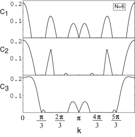
Figure 1: Concurrence between spins 1 and 2 (top), 1 and 3 (middle), and 1 and 4 (bottom) in a two-magnon scattering state $|\psi(0,k,0)\rangle$ of the six-spin Heisenberg chain. The relative pseudomomentum $k$ is treated as a continuous variable parameterizing states of the scattering form (Eq. II); $\phi_{12}$ is set to zero. Eigenstates occur at $k=2\pi\lambda_{2}/N$, $\lambda_{2}=0,\ldots,5$, and are indicated by ticks on the $k$-axis.

It is possible to prove analytically that this must always occur whenever a Goldstone and a non-Goldstone magnon mix. Choose two arbitrary spins $p<q$ of the HSC and trace out the rest: this yields the reduced density matrix $\rho(p,q)$, whose elements are (in the notation of Eq. 2):

$$\alpha(p,q) = \frac{4}{N(N-2)}c^{2}(\lambda_{2})$$ (14)

$$\beta(p,q) = \delta(p,q)=\frac{2}{N(N-2)}\left(N-2-2c^{2}(\lambda_{2})\right)$$ (15)

$$\gamma(p,q) = \frac{2(N-4)}{N(N-2)}\exp\left(\pi i(p-q)\lambda_{2}/N\right)c(\lambda_{2})$$ (16)

$$\epsilon(p,q) = \frac{1}{N(N-2)}\left((N-2)(N-4)+4c^{2}(\lambda_{2})\right),$$ (17)

where

$$c(\lambda_{2})=\cos\left(\frac{\pi\lambda_{2}(p-q)}{N}\right),$$ (18)

and $\lambda_{2}\in\{1,\ldots,N-1\}$ (these matrix elements are not correct when $\lambda_{2}=0$). The concurrence between spins $p$ and $q$, from Eq. 3, is

$$C(p,q)=\frac{4|c(\lambda_{2})|}{N(N-2)}\times$$ (19)

$$\max\left(0,N-4-\sqrt{(N-2)(N-4)+4c^{2}(\lambda_{2})}\right).$$

But

$$\sqrt{(N-2)(N-4)+4c^{2}(\lambda_{2})} > \sqrt{(N-2)(N-4)}$$ (20)

$$> N-4$$

for $N\geq 4$ and hence $C(p,q)$ is identically zero.

Because the two-magnon state under consideration (Eq. 13) is pure, the entanglement of formation $S_{f}$ for the reduced density matrix $\rho(p,q,r,\ldots)$ of any subset $p,q,r,\ldots$ of the spins of the HSC coincides with the binary von Neumann entropy of that density matrix: $S_{f}=-\textrm{Tr}\left[\rho(p,q,r,\ldots)\textrm{lg}\rho(p,q,r,\ldots)\right]$, where ${\textrm{lg}}(z)=\log_{2}(z)$. In particular, the entanglement of formation for the state of a single spin $p$ is simply

$$S_{f}=-\left(\frac{2}{N}\right)\textrm{lg}\left(\frac{2}{N}\right)-\left(1-\frac{2}{N}\right)\textrm{lg}\left(1-\frac{2}{N}\right).$$ (21)

This is nonzero for any finite $N>2$. These results yield the somewhat paradoxical conclusion that in states containing both a Goldstone and a non-Goldstone magnon, any specific spin is not entangled with any other spin individually, although it is entangled with all other spins collectively.

III.2 Multimagnon entanglement quenching

Suppose that a third magnon is excited on a HSC initially in a two-magnon entanglement-quenched state (Eq. 13). Will this create qubit entanglement? Again we can begin with the special case in which the additional magnon is also a Goldstone excitation. Three-magnon state vectors are somewhat difficult to manipulate analytically. They can however be generated with arbitrary precision using a numerical implementation of the Bethe Ansatz, and the partial trace required to find the two-spin RDM and the concurrence can then be done numerically with no loss of accuracy. All possible concurrences in all states describing the simultaneous excitation of two Goldstone and one non-Goldstone magnons for Heisenberg spin chains of lengths from $N=6$ to $N=50$ were calculated in this manner and found to be zero. Thus a second Goldstone magnon cannot revive quenched entanglement.

A different situation arises when two non-Goldstone magnons are present. Such states have complex entanglement structures, as will be discussed later. Table 1 shows the effects of the excitation of a Goldstone mode on qubit entanglement in the two-magnon scattering and bound states of an $N=6$ ring (in this case the BAE can be handled analytically). In five of the states entanglement is completely quenched. In two of the bound states (quantum numbers $\lambda_{1}=\lambda_{2}=1\ \textrm{or}\ 5$) the qubit entanglement is reduced, but not eliminated, while in two of the scatting states ($\lambda_{1}=1$, $\lambda_{2}=5$ and $\lambda_{1}=2$, $\lambda_{2}=4$), entanglement is actually generated at the longest range (i.e. $C_{3}$). Nevertheless, the total entanglement, as measured by the sum of the concurrences $C_{i}$, has decreased. This phenomenon is confirmed by numerical studies of other rings: excitation of a Goldstone magnon will occasionally generate entanglement between a formerly unentangled pair, but the total entanglement of the HSC is always reduced.

Finally, we consider entanglement quenching in the four-magnon case. Suppose a second Goldstone magnon is excited on a ring with two non-Goldstone and one Goldstone magnons. Numerical examination of all pairs of spins for Heisenberg spin chains of lengths from $N=8$ to $N=20$ show that all concurrences vanish in such states. Concurrence is also absent from these chain in all states with three Goldstone and one non-Goldstone magnons. These results, and those of the preceeding section, support the following hypothesis: the addition of a Goldstone excitation to a state containing one or more non-Goldstone magnons always reduces the total qubit entanglement in the HSC; and when the number of Goldstone magnons equals or exceeds the number of non-Goldstone excitations, there is no qubit entanglement whatsoever.

$\lambda_{1}$	$\lambda_{2}$	$C_{1}$	$C_{2}$	$C_{3}$	$C_{1}$	$C_{2}$	$C_{3}$
1	3	0.45	0	0	0	0	0
1	4	0.04	0	0	0	0	0
1	5	0	0.10	0	0	0	0.06
2	4	0.43	0	0	0.21	0	0.06
2	5	0.04	0	0	0	0	0
3	5	0.45	0	0	0	0	0
1	1	0	0.28	0.35	0	0	0.15
4	5	0	0.34	0	0	0	0
5	5	0	0.28	0.35	0	0	0.15

Table 1: Partial quenching of entanglement. $\lambda_{1}$ and $\lambda_{2}$ are the quantum numbers of two non-Goldstone magnons on a six-spin HSC. Concurrences $C_{i}$ are shown without (center column) and with (right column) an additional Goldstone magnon. The first six entries are scattering states, while the next three are bound states.

IV The pure Goldstone sector

As remarked previously and illustrated in Table. 1, the excitation of second Goldstone magnon from a single-Goldstone state reduces but does not completely quench qubit entanglement. Thus from the standpoint of entanglement behavior, the pure Goldstone sector is fundamentally different from the mixed sector. As further Goldstone magnons are excited, the qubit concurrence continues to decrease without vanishing. There is no length scale associated with these Goldstone magnons (because their pseudomomentum is zero), and the HSC qubits remain equientangled in all states comprised entirely of Goldstone excitations. This situation can be studied analytically. The general formula for the concurrence between any two qubits in an $n$-Goldstone state of an $N$-qubit ring is

$$C(n,N)=\frac{2}{N(N-1)}\times$$ (22)

$$[n(N-n)-\sqrt{n(n-1)(N-n)(N-n-1)}].$$

This result has been derived elsewhere, and its implications for thermal entanglement have been discussed Pratt . When $n=0$ or $n=N$, the eigenstate corresponds to all spins pointing down (the state $|\emptyset\rangle$) or all spins pointing up, and hence is factorable. Maximal entanglement occurs when a single magnon is excited with respect to either of these states, i.e. $n=1$ or $n=N-1$. Excitation of a second Goldstone magnon produces a large relative decline in entanglement, but thereafter qubit entanglement is only weakly dependent on the number of Goldstone magnons excited, as shown in Fig. 2.

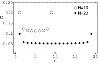
Figure 2: Concurrence between any two qubits in a $N$-spin Heisenberg chain as a function of the number $n$ of Goldstone magnons present.

Figure 3: (right) Contour plots of concurrences between spins 1 and 2 ($C_{1}$), spins 1 and 3 ($C_{2}$), etc., for two-magnon scattering states (Eq. II) of an 8-spin HSC, as functions of the relative pseudomomentum $k$ and the Bethe phase $\phi=\phi_{12}$. White regions denote zero concurrence; contours are evenly spaced at intervals of 0.05 (top two graphs), 0.03 (third graph), and 0.01 (bottom graph). Values of $(k,\phi)$ corresponding to energy eigenstates are indicated by dots. Small dots denote a single eigenstate. The six large dots denote two eigenstates with the same $(k,\phi)$ values and hence the same entanglement; such a pair need not be energetically degenerate. (Note that near $k\approx 1,\phi\approx 2.5$ a single state and a double state nearly coincide.) The point at $(0,0)$ is the eigenstate containing two Goldstone magnons. The seven eigenstates with one Goldstone magnon form a row on the $\phi$–axis. In the $C_{4}$ plot the dotted lines (for example, bisecting the central “islands”) are zero-entanglement boundaries between two entangled regions.

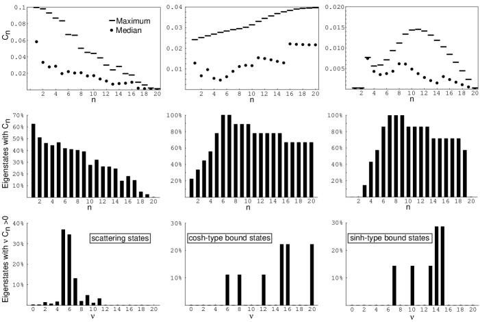
Figure 4: Statistical characterization of entanglement in two-magnon states for the $N=40$ HSC. Left column: scattering eigenstates. Center column: $\cosh$-type bound eigenstates. Right column: $\sinh$-type bound eigenstates. The upper graphs show the maximum concurrence at a qubit separation $n$ among all eigenstates in the indicated population, and the median concurrence of the subpopulation of states with nonzero $C_{n}$. The middle graphs show the percentage of two-magnon eigenstates with nonzero $C_{n}$ as a function of $n$. The lower graphs show the percentage of two-magnon scattering states states with exactly $\nu$ values of $C_{n}$ not equal to zero.

V The Goldstone-free sector

V.1 Two-magnon scattering states

The previous sections have characterized qubit entanglement in the pure Goldstone and the mixed Goldstone/non-Goldstone sectors of the HSC. We now consider the pure non-Goldstone sector, beginning with the two-magnon states. For scattering states (Eq. II) it is easy to show that the concurrence depends only on the relative pseudomomentum $k$ and the Bethe phase $\phi$, and not on the total pseudomomentum $K$. We can plot the concurrence as a function of these variables unconstrained by the BAE (Eq. 5). This is shown in Fig. 3 for the $N=8$ case, with the eigenstates (those parameter values which do satisfy the BAE) indicated by dots. The fifteen zero-Goldstone states form an irregular wedge in the upper half-plane. The double-Goldstone state and the single-Goldstone states appear as a row on the $\phi$–axis. As in Fig. 1, the positioning of these latter states is striking: although always unentangled, they often lie near or on the boundaries of regions of entanglement, so that a slight perturbation of the Bethe parameters would yield an entangled state. There is no relation between an eigenstate’s entanglement and its eigenenergy (which, unlike its concurrences, depends on the total pseudomomentum), and, as the complexity of the concurrence diagrams suggests, there is no simple relationship between entanglement and the Bethe parameters.

Although qubit entanglement cannot easily be calculated directly in terms of the Bethe parameters for non-Goldstone multimagnon states, the Bethe Ansatz classification partitions eigenstates into populations with statistically distinct patterns of qubit entanglement. In the two-magnon case, the scattering states are characterized qualitatively by short-range entanglement, which distinguishes them from the bound states. There are a number of ways to make this observation quantitative. One way is to ask about the maximum concurrence attained by any scattering state as a function of qubit separation. As shown in Fig. 4 for the $N=40$ case, this maximum decreases roughy linearly (but nonmonotonically) with increasing qubit separation, and in fact is exactly zero at the longest range ($C_{20}$), that is, between opposite spins on the Heisenberg chain. This is not simply due to outlying extreme values. If one culls the total population of two-magnon scattering states, and calculates the median concurrence as a function of qubit separation $n$ among those states with nonzero $C_{n}$, the median of each subpopulation is typically between one-half and one-third of the maximum. Another measure of the short-range nature of entanglement is the decline in the number of eigenstates with nonzero concurrence as a function of distance. Over $60\%$ of scattering states have nearest-neighbor entanglement; this decays roughly linearly with increasing qubit separation, and as already noted becomes zero at the longest range. Most two-magnon scattering states have entanglement at only a few different distances, usually only $5$ or $6$; no scattering state has more than $11$ nonzero values of $C_{n}$. Similar observations hold for other values of $N$.

Examination of $C_{4}$ entanglement in Fig. 3 (where $N=8$) shows that all the scattering states lie in regions of zero concurrence. Similarly, inspection of Table 1 shows that $C_{3}$ vanishes for scattering states when $N=6$. Analytic calculations showed that $C_{2}$ was always zero for scattering states when $N=4$ or $5$, and $C_{20}$ was seen above to vanish when $N=40$. These observations suggested the hypothesis that concurrence at the longest range, $C_{\lfloor N/2\rfloor}$, is always zero for two-magnon scattering states. All such states for $N=4$ up to $N=50$ were generated numerically, and $C_{\lfloor N/2\rfloor}$ always equalled zero as conjectured. This is yet another manifestation of the short-range nature of scattering state entanglement.

V.2 Two-magnon bound states

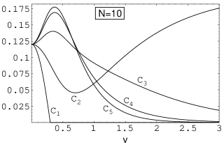
Figure 5: Nearest-neighbor concurrence $C_{1}$, next-nearest-neighbor concurrence $C_{2}$, etc., for $\cosh$-type bound (CB) states in the 10-spin Heisenberg chain. Two eigenstates occur at $v=0.258$ and two at $v=1.174$. An ‘anomalous’ regime, in which entanglement increases with qubit separation, extends to about $v\approx 0.7$.

In contrast to the scattering states, the two-magnon bound states are characterized by long-range entanglement. The behavior of the $\cosh$-type (Eq. II) and $\sinh$-type (Eq. II) states is similar but distinct. Analogous to the independence of scattering state entanglement from the total pseudomomentum $K$, bound state entanglement is easily shown to be independent of the phase parameter $u$; qubit concurrence is controlled entirely by the binding parameter $v$. This dependence can be plotted by treating $v$ as a continuous parameter unconstrained by the BAE (Eq. 5), as shown in Fig. 5 for the CB states and in Fig. 6 for the SB states for a 10-spin HSC. In the limit $v\rightarrow 0$, the CB state becomes the two-Goldstone state and all concurrences are equal. As $v$ increases, the short-range components of entanglement, $C_{1}$ and $C_{2}$, fall off, while the longer-range components increase. In this low-$v$ ‘anomalous’ parameter regime $C_{n}$ increases with $n$, that is, spins actually become more highly entangled with increasing separation. As $v$ continues to increase, $C_{1}$ becomes identically zero, and never revives. $C_{2}$ passes through a minimum and rises to become the dominant component, and the order of the strengths of the longer-range concurrences undergoes an inversion, so that entanglement now falls off with increasing spin separation. Asymptotically, as $v\rightarrow\infty$, all concurrences vanish except for $C_{2}$, whose limit will be calculated below. Similar features occur for longer-$N$ spin chains; in particular, there is always an ‘anomalous’ region for small $v$.

The physical implications of this for eigenstates are determined by the distribution of solutions to the BAE (Eq.5), which for the CB states can be rewritten as

$$\coth\left(\frac{Nv}{2}\right)=\frac{\sinh v}{\cosh v-\cos\left(\frac{\pi\lambda}{N}\right)},$$ (23)

where $\lambda$ is a quantum number. Numerically, it is found that the roots (values of $v$ corresponding to eigenstates) of this equation always lie between $N^{-3/2}$ (a strict lower bound) and $\ln(N)$ (a strict upper bound), with one exception which will be described below; further, the roots are strongly clumped towards the lower bound. The result is that most allowed $v$-values actually lie in the anomalous parameter region where entanglement strength increases with qubit separation; this becomes more pronounced as $N$ increases. This is reflected in the statistics of the CB state population, as shown in Fig. 4. In general, CB states are much more entangled than scattering states; for example, nearly a quarter of the CB states have nonzero concurrence at every length scale. The magnitude of the concurrences, however, is typically smaller for bound states than for scattering states.

When $N>2$ is even, but not when $N$ is odd, there is one solution of the two-magnon BAE in which the pseudomomenta have infinite imaginary parts Siddharthan . This is the exception mentioned above, corresponding to $v\rightarrow\infty$. This eigenstate with singular Bethe parameters is:

$$|\psi_{\infty}\rangle=\frac{1}{\sqrt{N}}\sum_{m=1}^{N}(-1)^{m+1}|m,m+1\rangle.$$ (24)

It is the maximally bound state; the two inverted spins are always adjacent. Formally, it is a CB state when $N/2$ is even and an SB otherwise. When all spins except $p$ and $q$ are traced out, the elements of the RDM are

$$\alpha(p,q) = \frac{1}{N}\delta_{p+1,q}$$ (25)

$$\beta(p,q) = \delta(p,q)=\frac{1}{N}(2-\delta_{p+1,q})$$ (26)

$$\gamma(p,q) = \frac{-\delta_{p+2,q}-\delta_{N,4}}{N}$$ (27)

$$\epsilon(p,q) = \frac{N-4+\delta_{p+1,q}}{N},$$ (28)

where $\delta_{ij}$ is the Kronecker delta. The concurrence is therefore

$$C_{r}=\left(\frac{2+2\delta_{N,4}}{N}\right)\delta_{r,2}.$$ (29)

Thus there is an unusual entanglement pattern, with no entanglement except between next-nearest-neighbors, whose concurrence is simply $2/N$ if $N>4$. The four-spin ring is exceptional; opposite corner qubits are perfectly entangled. Intuitively, diagonal qubits are next-nearest-neighbors on both sides (in both directions around the ring). It is striking that the $v\rightarrow\infty$ limit is realized by a physical eigenstate.

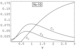
Figure 6: Next-nearest-neighbor concurrence $C_{2}$, etc., for $\sinh$-type bound (SB) states in the 10-spin Heisenberg chain. Two eigenstates occurs at $v=0.521$; the singular state (Eq. 24) lies at $v=\infty$. Note the absence of both nearest-neighbor ($C_{1}$) and longest-range ($C_{5}$) entanglement.

There are several notable differences that distinguish the CB and SB bound states. First, in SB states nearest-neighbor entanglement is always identically zero. This can be proven analytically, by a method resembling that used for the proof of Goldstone-mediated entanglement quenching given above, but computationally much more involved. Second, when $N$ is even, longest-range entanglement $C_{N/2}$ is also identically zero. The result follows immediately from calculating that the coherence $\gamma$ (notation of Eq. 2) vanishes for opposite spins, irrespective of the value of $v$. Thus SB state entanglement exhibits a sensitivity to the parity of $N$ that CB states do not. Most significantly, however, the anomalous parameter regime does not in general exist for SB states; rather, at $v=0$, the maximum concurrence typically lies at some intermediate range, so that $C_{N/4}$ (or thereabouts) is the dominant form of entanglement. As $v$ increases, the concurrence curves cross at irregular intervals. The values of $v$ corresponding to eigenstates are constrained by the BAE:

$$\tanh\left(\frac{Nv}{2}\right)=\frac{\sinh v}{\cosh v-\cos\left(\frac{\pi\lambda}{N}\right)}.$$ (30)

As with Eq. 23, the roots cluster strongly at small $v$ values, and the eigenstate entanglement statistics (Fig. 4, right column) reflect the dominance of intermediate-range entanglement. Thus the various classes of two-magnon eigenstates as determined by the Bethe Ansatz exhibit distinct patterns of entanglement behavior.

V.3 Multimagnon states

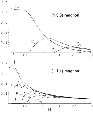
Figure 7: Qubit concurrences in the three-magnon pure scattering eigenstate with quantum numbers $\vec{\lambda}=(1,3,5)$, and in the three-magnon pure bound eigenstate with quantum numbers $\vec{\lambda}=(1,1,1)$, as functions of the HSC length $N$. Curves are drawn continuously for visual clarity, but only values at integral $N$ are meaningful. The notation $C_{-i}$ is used to denote the concurrence $C_{\lfloor N/2\rfloor+1-i}$, that is, $C_{-1}$ is the concurrence at the longest range (between opposite qubits on the ring), $C_{-2}$ is the concurrence at the next-longest range, etc. The (1,1,1)-magnon has shorter-range concurrences (lower $C_{-i}$ components) which are not shown.

The entanglement characteristics of two-magnon bound and scattering states generalize to multimagnon states. For example, the quantum numbers $\vec{\lambda}=(\lambda_{1},\lambda_{2},\lambda_{3})=(1,3,5)$ specify a pure scattering state of three magnons with real pseudomomenta for any chain length $N\geq 6$, while $\vec{\lambda}=(1,1,1)$ always corresponds to a pure bound state, i.e. a three-magnon wavecomplex. The entanglement behaviors of these eigenstates are shown in Fig. 7. The scattering state has only nearest-neighbor entanglement up to $N=12$; next-nearest-neighbor entanglement does not become dominant until $N=17$, and $C_{3}$ entanglement arises only at $N=20$. Thus, qualitatively, the range of nonzero entanglement is always much smaller than the longest range possible. This behavior is typical of all pure scattering multimagnon states studied so far. In contrast, the wavecomplex state initially ($N=6$) has only longest range entanglement (written as $C_{-1}$, as explained in the caption for Fig. 7); next-longest range entanglement $C_{-2}$ arises at $N=8$, and by $N=16$ entanglement is present at every range. However, the magnitude of the concurrence always increases as qubit separation increases, just as for a two-magnon CB state in the ‘anomalous’ regime. Thus the entanglement patterns observed in the two-magnon case also occur in multimagnon bound and scattering states.

Of particular interest is the behavior of the antiferromagnetic ground state (AGS), which for even-$N$ chains is nondegenerate. In the BA formalism the AGS is specified by the quantum numbers $\vec{\lambda}=(1,3,\ldots,N-1)$ and is a pure scattering state. It has been proven by O’Connor and Wootters O'ConnorWootters that of all even-$N$ translationally invariant states with $S^{z}=0$, the AGS has maximal nearest-neighbor concurrence. To study this further, the AGS was calculated analytically for $N=4,6$ and numerically for $N=8,10,12$ (work is underway to study longer HSCs). Two new results were obtained. First, all concurrences except $C_{1}$ vanished; that is, the AGS appears (based on these few cases) to have only nearest-neighbor entanglement, as one might anticipate for a pure scattering state with the maximum number of magnons possible. More generally, no examples have been found of a chain with $\lfloor N/2\rfloor$ scattering magnons having any qubit concurrence beyond nearest-neighbor, although this work is preliminary. Second, while the AGS does indeed have the largest nearest-neighbor entanglement, other translationally invariant $S^{z}=0$ eigenstates can have much stronger entanglement at longer ranges. For example, the 6-spin AGS $\vec{\lambda}=(1,3,5)$ has $C_{1}=0.43456$, but the bound state $\vec{\lambda}=(1,1,1)$ has $C_{3}=0.70313$.

VI Discussion

The Bethe Ansatz provides a method for describing eigenstates of the Heisenberg spin chain in terms of their pseudoparticle content. This paper has shown that the natural classification of eigenstates originating in this description predicts qualitatively and sometimes quantitatively the qubit entanglement of these states. Magnons with zero pseudomomentum, here termed Goldstone magnons, effectively reduce or suppress entanglement relative to the corresponding Goldstone-free state. From an applied point of view this is a form of noise which may affect the processing, storage or coherent transmission of quantum information in exchange-coupled qubits PrattEberly . Pure scattering states are composed of one or more magnons with real pseudomomenta. While a single such magnon leads to qubit equientanglement, the presence of additional scattering magnons favors short-range entanglement: statistically, qubit entanglement becomes both weaker and less common in the population of scattering states as interqubit separation increases. In particular, the antiferromagnetic ground state seems to exhibit only nearest-neighbor entanglement. In contrast, bound states consist of two or more magnons with complex pseudomomenta. For a pair of bound magnons qubit entanglement is controlled solely by the binding parameter $v$ and the interqubit separation. In the large-$v$ limit next-nearest-neighbor entanglement approaches $2/N$, while all other forms of entanglement approach zero. This $v\rightarrow\infty$ limit is actually realized in even-$N$ spin chains by the singular state. Most nonsingular two-magnon bound states have small values of $v$; in this binding parameter regime the order of the concurrence curves is inverted for $\cosh$-type states, so that entanglement increases with qubit separation, while in $\sinh$-type bound states entanglement at intermediate lengths is favored statistically. Behavior similar to that of the $\cosh$-type states is seen in multimagnon bound states such as the three-magnon $\vec{\lambda}=(1,1,1)$ state. Multi-wavecomplex states, comprised of magnons bound into groups which are not bound to one another (e.g. a four-magnon state of two bound pairs), remain to be studied, as do mixtures of scattering magnons and wavecomplexes.

The outstanding question at this point is whether this approach to understanding entanglement via the Bethe Ansatz can be extended to other models. The BA can also be used to solve other spin-$1/2$ chains, such as the anisotropic deformations of the HSC (e.g. the XXZ and XYZ models), and it will be interesting to see if the same features, such as short-range entanglement in scattering states, reappear. More challenging is the extension of this approach to Hamiltonians which include hopping, such as the one-dimensional Hubbard model, which are solved by the so-called nested Bethe Ansatz LiebWu . If similar features do reappear, as seems plausible, it may reflect a kind of universality arising from the BA structure of the solutions, allowing us to predict aspects of entanglement behavior across a broad range of physical systems.

References

- (1) T.M. Forcer, A.J.G. Hey, D.A. Ross, and P.G.R. Smith, Quant. Info. and Comp. 2, 97 (2002).
- (2) C.H. Bennett and S.J. Wiesner, Phys. Rev. Lett. 69, 2881 (1992).
- (3) Z.Y. Ou and L. Mandel, Phys. Rev. Lett. 61, 50 (1988).
- (4) Michael Keyl, Physics Reports 369, 431 (2002).
- (5) Asher Peres and Daniel R. Terno, Rev. Mod. Phys. 76, 93 (2004).
- (6) C.K. Law and J.H. Eberly, Phys. Rev. Lett. 92, 127903 (2004).
- (7) M.C. Arnesen, S. Bose, and V. Vedral, Phys. Rev. Lett. 87, 017901 (2001).
- (8) T.J. Osborne and M.A. Nielsen, Phys. Rev. A 66, 032110 (2002); A. Osterloh, L. Amico, G. Falci, and R. Fazio, Nature 416, 608 (2002); J.I. Latorre, E. Rico, and G. Vidal, Quant. Info. Comp. 4, 048-092 (2004).
- (9) D. Gunlycke, V.M. Kendon, V. Vedral, S. Bose, Phys. Rev. A 64 042302 (2001); G.L. Kamta and A.F. Starace, Phys. Rev. Lett. 88, 107901 (2002).
- (10) H. Bethe, Z. Physik 71, 205 (1931).
- (11) S. Hill and W.K. Wootters, Phys. Rev. Lett. 78, 5022 (1997); W.K. Wootters, Phys. Rev. Lett. 80, 2245 (1998); W.K. Wootters, Quant. Info. Comp. 1, 27 (2001).
- (12) J. Goldstone, A. Salam, and S. Weinberg, Phys. Rev. 127, 965 (1962).
- (13) J.S. Pratt, in preparation.
- (14) R. Siddharthan, cond-mat/9804210 (1998).
- (15) Kevin M. O’Connor and William K. Wootters, Phys. Rev. A 63, 052302 (2001).
- (16) J.S. Pratt and J.H. Eberly, Phys. Rev. B 64, 195314 (2001).
- (17) E. Lieb and F.Y. Wu, Phys. Rev. Lett. 20, 1445 (1968).