Optical analog of Rabi oscillation suppression due to atomic motion

Abstract

The Rabi oscillations of a two-level atom illuminated by a laser on resonance with the atomic transition may be suppressed by the atomic motion through averaging or filtering mechanisms. The optical analogs of these velocity effects are described. The two atomic levels correspond in the optical analogy to orthogonal polarizations of light and the Rabi oscillations to polarization oscillations in a medium which is optically active, naturally or due to a magnetic field. In the later case, the two orthogonal polarizations could be selected by choosing the orientation of the magnetic field, and one of them be filtered out. It is argued that the time-dependent optical polarization oscillations or their suppression are observable with current technology.

I Introduction

The analogies between phenomena occurring in two different physical systems open a route to find new effects or to translate solution techniques or devices, and quite often help to understand both systems better. The parallelism between light and atom optics, in particular, has been a strong driving force for fundamental and applied research, and it has received recently renewed impulse with the advent of laser cooling techniques, and Bose-Einstein condensation of alkali gases. Atomic interferometers or atom lasers are important examples that illustrate the fruitfulness of this correspondence.

The analogy may also enable us to perform in one system experiments which are difficult to carry out in the other one. As an example, tunneling time experiments are much easier for microwaves than for matter waves tqm12 ; tqm11 . Typically, optical analogs of quantum mechanical matter wave effects, if available, are simpler and less costly to implement than their matter counterparts. In addition, the electromagnetic pulses can be probed in a non-invasive way.

In this paper we shall describe the optical analogs of the time-dependent atomic Rabi oscillation in a laser field and of several dynamical suppression effects due to quantum, pure state atomic motion. The Rabi oscillation is at the heart of measurement procedures for time and frequency standards Ramsey , photon number in a cavity Haroche , and other metrological applications ai ; DEHM02 , so its dynamic suppression may be a relevant effect, in particular for atomic clocks; This suppression has been also proposed as a way to prepare specific internal atomic states by projection in quantum information applications NEMH03 .

The relation between light and atom optics is frequently established at the level of translational (external) degrees of freedom, but here we need, in addition, an optical parallel of the two internal levels of the atom, which is provided by the orthogonal states of light polarization. Thus we follow in reverse order, from matter to light, a connection that can be traced back historically to early experiments of I. Rabi, later modified by N. F. Ramsey, which lead to the development of atomic clocks, and provided atomic analogs of polarization interferometry in optics, with the internal states of the atom or molecule playing the role of the polarization states of the photon Ramsey .

For completness a brief review of the dynamical suppression of the Rabi oscillation is provided in section II, which is mostly based on ref. NEMH03 but incorporates also some new elements; Section III is devoted to the description of the optical analog, Section IV presents numerical illustrations, and Section V describes a possible implementation of polarization filtering making use of magnetic fields.

II Rabi oscillation suppression for moving atoms

Neglecting decay, the effective Hamiltonian for a two level atom at rest and in presence of a detuned laser field is

$$H=\frac{\hbar}{2}\left({0\atop\Omega^{*}}{\Omega\atop-2\delta}\right),$$ (1)

where $\Omega$ is the on-resonance Rabi frequency, $\delta=\omega_{L}-\omega$ is the detuning ($\omega_{L}$ being the laser frequency and $\omega$ the atomic frequency) and internal ground and excited states are represented as $|1\rangle\equiv{1\choose 0}$ and $|2\rangle\equiv{0\choose 1}$, respectively. If at time zero the atom is in the ground state, the ground and excited components of the state evolved with this Hamiltonian are

$$\psi^{(1)} = e^{i\delta t/2}[\cos(\Omega^{\prime}t/2)-(i\delta/\Omega^{\prime})\sin(\Omega^{\prime}t/2)],$$ (2)

$$\psi^{(2)} = e^{i\delta t/2}[(-i\Omega/\Omega^{\prime})\sin(\Omega^{\prime}t/2)],$$ (3)

so that the populations $|\psi^{(1,2)}|^{2}$ alternate oscillating harmonically in time with “Rabi period” $2\pi/\Omega^{\prime}$ and effective Rabi frequency $\Omega^{\prime}\equiv(\delta^{2}+|\Omega|^{2})^{1/2}$. The oscillation may however be suppressed when the atoms move into a region illuminated by a perpendicular laser beam NEMH03 . For an idealized sharp laser profile in a one dimensional approximation (its validity and the three dimensional case are examined in HHM05 ), the Hamiltonian becomes

$$H={\widehat{p}}^{2}/2m+\frac{\hbar}{2}\Theta({\widehat{z}})\left({0\atop\Omega^{*}}{\Omega\atop-2\delta}\right),$$ (4)

where $\widehat{z}$ and $\widehat{p}$ are position and momentum operators. If reflection is negligible, for moderate to high velocities, the stationary wave for incidence in the ground state with wavenumber $k$ can be approximated, up to a normalization constant, as

$\phi_{k}^{(1)}\approx e^{ikz}e^{i\delta t/2}\bigg{[}\cos\left(\frac{\Omega^{\prime}zm}{2\hbar k}\right)-(i\delta/\Omega^{\prime})\sin\left(\frac{\Omega^{\prime}zm}{2\hbar k}\right)\bigg{]},$

$\phi_{k}^{(2)}\approx e^{ikz}e^{i\delta t/2}\bigg{[}(-i\delta/\Omega^{\prime})\sin\left(\frac{\Omega^{\prime}zm}{2\hbar k}\right)\bigg{]}.$
This may be interpreted semiclassically as the state of an ensemble of independent atoms which travel with momentum $k\hbar$ and sustain Rabi oscillations. Note that the quantity $zm/\hbar k$ plays the role of time in the arguments of the trigonometric functions, compare with Eqs. (2) and (3). In other words, the Rabi oscillation is also evident spatially in the stationary waves, under the form of density undulations of the two components with a “Rabi wavelength” $\lambda_{R}=kh/m\Omega^{\prime}$.

The Rabi oscillation may be suppressed “adiabatically” if a quasi-monochromatic, pure-state wave packet enters slowly into the laser illuminated region. Intuitively, and according to a classical picture, the atoms in the ensemble start to oscillate at different times because of their different entrance instants, so the global oscillation averages out if the entrance interval of the packet is greater than the Rabi oscillation period. This intuitive interpretation cannot be taken too literally though. In particular, the suppression involves a pure state and not a statistical mixture. Note also that no incoherent “fading” due to decay from the excited state is involved. (The effect of fading was discussed in NEMH03 .)

A second group of suppression effects is associated with state filtering or velocity splitting. To explain these two related concepts, we need a more accurate representation than before. In the laser region, let $|\lambda_{+}\rangle$ and $|\lambda_{-}\rangle$ be the eigenstates, corresponding to the eigenvalues $\lambda_{\pm}$, of the matrix $\frac{1}{2}\left({0\atop\Omega^{*}}{\Omega\atop-2\delta}\right)$. One easily finds

$$\lambda_{\pm} = \frac{-\delta\pm\Omega^{\prime}}{2},$$ (5)

$$|\lambda_{\pm}\rangle = {1\choose\frac{-\delta\pm\Omega^{\prime}}{\Omega}},$$ (6)

where $|\lambda_{\pm}\rangle$ have not been normalized. [For later comparison with “circularly polarized states” notice that by setting $\delta=0$ and for the case $\Omega$=i$|\Omega|$, $\lambda_{\pm}=\pm\frac{\Omega}{2}$, and $|\lambda_{\pm}\rangle={1\choose\mp i}$.] The stationary state for $z>0$ can be written as a superposition

$$\Phi_{k}(z)=C_{+}|\lambda_{+}\rangle e^{ik_{+}z}+C_{-}|\lambda_{-}\rangle e^{ik_{-}z},$$ (7)

where

$$k_{\pm}=k\left(1-\frac{m(-\delta\pm\Omega^{\prime})}{\hbar k^{2}}\right)^{1/2},$$ (8)

and the coefficients $C_{\pm}$ are obtained from the matching conditions at $z=0$ NEMH03 . The two components $(\pm)$ have two different propagation velocities and in fact the Rabi oscillation may be understood as an interference between the two terms when $k_{\pm}\approx k+m(\delta\mp\Omega^{\prime})/(2\hbar k)$. For initially quasimonochromatic packets, with the wavenumber spread much smaller than the average wavenumber, $\sigma_{k}/k_{0}\ll 1$, the two different velocities also imply eventually a spatial separation of the $|\lambda_{\pm}\rangle$ components, so that the interference and associated Rabi oscilation finally disappear for times larger than the time to split the packet into two, $2\sigma_{z}k/\Omega^{\prime}$, where $\sigma_{z}^{2}$ is the spatial variance of the wave packet. An extreme case is the complete state filtering that occurs for very low kinetic energies, when $k_{-}$ is purely imaginary so that $e^{ik_{-}z}$ becomes an evanescent wave and only the $|\lambda_{+}\rangle$ component survives in the laser region for $z$ greater than the penetration length $[{\rm Im}(k_{-})]^{-1}$. Since the exact form of the surviving $|\lambda_{+}\rangle$ state can be modified by the laser detuning and Rabi frequency, this state filtering effect provides a projection mechanism to prepare especific internal states regardless of the incident atomic state NEMH03 .

III Optical analog

In the optical analog of the dynamic effects described, the internal states will be substituted by orthogonal polarizations of the field, and the laser region by an optically active medium; the rotation of the polarization plane and corresponding oscillation of the linear polarization intensities will mimic the Rabi oscillation, and electromagnetic pulses will play the role of the atomic wave packets.

The use of a complex electric field for quasi-monochromatic pulses within analytic signal theory facilitates the comparison and correspondence between quantum wave function and electric field components. Some of the parallelisms are quite direct. For example, we shall keep the same notation for the quantum wavenumbers and the optical propagation constants $k$ and $k_{\pm}$, or for the coefficients in the stationary waves, such as $C_{\pm}$ and the reflection amplitudes $R$, although their values and detailed expressions need not be equal. Atomic populations in the ground state may be related to total energies in the vertical, linear polarization component and, similarly, the atomic excited state will be mimicked by horizontal, linear polarization. In our analogy, positions and times are present both in optics and quantum mechanics since we want to describe and compare pulses and wavepackets in space-time. This is at variance with the analogy established by Zaspasskii and Kozlov ZK , in which the spatial coordinate played the role of time in a Schrödinger-like equation satisfied by the polarization vector.

III.1 Basic relations

From the Maxwell equations in a nonmagnetic, electrically neutral dielectric medium, the wave equation for the ${\bf E}$ field is

$$\nabla\times(\nabla\times{\bf E})+\frac{1}{c^{2}}\frac{\partial^{2}{\bf E}}{\partial t^{2}}=-\mu_{0}\frac{\partial^{2}{\bf P}}{\partial t^{2}},$$ (9)

where $\mu_{0}$ is the permeability of the vacuum, $c$ the speed of light in vacuum and ${\bf P}$ the macroscopic polarization (volume density of electric dipoles), which we assume to be given by the linear constitutive relation

$${\bf P}=\epsilon_{0}{\bm{\chi}}{\bf E},$$ (10)

where $\epsilon_{0}$ is the permittivity of the vacuum, and ${\bm{\chi}}$ is the susceptibility tensor

$${\bm{\chi}}=\left[\begin{array}[]{ccc}\chi_{11}&\chi_{12}&\chi_{13}\\ \chi_{12}^{*}&\chi_{22}&\chi_{23}\\ \chi_{13}^{*}&\chi_{23}^{*}&\chi_{33}\end{array}\right].$$ (11)

The medium is assumed to be non-absorbing so that ${\bm{\chi}}$ is hermitian. The absorbing case is briefly considered in section V and in the Appendix.

In the medium, $\bf{E}$ may not be perpendicular to the propagation direction but the electric displacement

$${\bf D}=\epsilon_{0}{\bf E}+{\bf P}$$ (12)

is perpendicular, since, from Eq. (9) and assuming a harmonic, plane wave solution $e^{i{\bf{k}}_{m}\cdot{\bf{r}}}e^{-i\omega t}$,

$${\bf k}_{m}\times({\bf k}_{m}\times{\bf E})=-\frac{\omega^{2}}{c^{2}\epsilon_{0}}{\bf D}.$$ (13)

The subscript $m$ in $k_{m}$ stands for “medium” and it will be used to avoid confusion with $k=\omega/c$ in vacuum. In components, and for ${\bf k}_{m}$ in $z$ direction, $D_{z}=0$ and

$${D_{x}}=\frac{c^{2}\epsilon_{0}k_{m}^{2}}{\omega^{2}}{E_{x}},\;\;\;{D_{y}}=\frac{c^{2}\epsilon_{0}k_{m}^{2}}{\omega^{2}}{E_{y}}$$ (14)

i.e., the displacement vector components whose ratio determines the polarization state of the harmonic wave, are proportional to the corresponding components of E. From Eqs. (10), (12), and (13),

$${\bf k}_{m}\times({\bf k}_{m}\times{\bf E})+\frac{\omega^{2}}{c^{2}}{\bf E}=-\frac{\omega^{2}}{c^{2}}{\bm{\chi}}{\bf E},$$ (15)

which, written in components leads to

$${E_{z}}=-(\chi_{13}^{*}{E_{x}}+\chi_{23}^{*}{E_{y}})/\gamma_{3}$$ (16)

and the system

$$\!\!\bigg{[}\!\!-\!\!k_{m}^{2}\!+\!\frac{\!w^{2}\!}{\!c^{2}\!}\!\left(\gamma_{1}\!-\!\frac{\!|\!\chi_{13}\!|^{2}\!}{\gamma_{3}}\!\right)\!\!\bigg{]}\!E_{x}\!\!+\!\!\frac{\!w^{2}\!}{\!c^{2}\!}\!\left(\!\chi_{12}\!-\!\frac{\!\chi_{13}\chi_{23}^{*}\!}{\gamma_{3}}\!\right)\!\!E_{y}\!=\!0,\!$$

$$\!\!\frac{\!w^{2}\!}{\!c^{2}\!}\!\!\left(\!\chi_{12}^{*}\!-\!\frac{\!\chi_{23}\chi_{13}^{*}\!}{\gamma_{3}}\!\right)\!\!E_{x}\!\!+\!\!\bigg{[}\!\!-\!k_{m}^{2}\!\!+\!\frac{\!w^{2}\!}{\!c^{2}\!}\!\left(\gamma_{2}\!-\frac{\!|\!\chi_{23}\!|^{2}\!}{\gamma_{3}}\!\right)\!\!\bigg{]}\!E_{y}\!\!=\!0,$$ (17)

where $\gamma_{j}\equiv 1+\chi_{jj}$. It can be solved by making the determinant of the coefficients vanish. The result is a fourth order equation ($k_{m}^{4}+\alpha k_{m}^{2}+\beta$=0) with coefficients

$$\alpha = \frac{-\omega^{2}}{c^{2}}\bigg{[}\gamma_{1}+\gamma_{2}-\frac{|\chi_{13}|^{2}+|\chi_{23}|^{2}}{\gamma_{3}}\bigg{]}$$ (18)

$$\beta = \frac{\omega^{4}}{c^{4}}\bigg{[}\gamma_{1}\gamma_{2}-\frac{\gamma_{2}|\chi_{13}|^{2}}{\gamma_{3}}-\frac{\gamma_{1}|\chi_{23}|^{2}}{\gamma_{3}}$$

$$+ \frac{|\chi_{13}|^{2}|\chi_{23}|^{2}}{\gamma_{3}}-\left|\chi_{12}-\frac{\chi_{13}\chi_{23}}{\gamma_{3}}\right|^{2}\bigg{]}.$$

Since we shall assume that the wave incides from a vacuum region adjacent to a semiinfinite medium, we only pick up two physical solutions (if complex they must have a positive imaginary part to decay; if real they must be positive to implement outgoing boundary conditions) and denote them as $k_{\pm}$,

$$k_{\pm}=\frac{\omega}{c}n_{\pm},$$ (20)

$n_{\pm}$ being the corresponding refraction index. Examples will be given soon.

The polarization corresponding to each solution in the $x-y$ plane, up to an intensity constant, may be given in terms of the Jones vector $\left[\begin{array}[]{c}E_{x}\\ E_{y}\end{array}\right]_{\pm}$ Fowles . For a closer comparison with the atomic case we may use the notation $E^{(1)}\equiv E_{x}$, $E^{(2)}\equiv E_{y}$, reminiscent of the atomic ground and excited state amplitudes. In particular, the internal atomic states $({1\atop 0})$ (ground) and $({0\atop 1})$ (excited) correspond to the Jones vectors $\left[\begin{array}[]{c}1\\ 0\end{array}\right]$, $\left[\begin{array}[]{c}0\\ 1\end{array}\right]$ which denote, respectively, “vertical” ($x$-direction) and “horizontal” ($y$-direction) linear polarization.

Since we are not specifying the total intensity, the polarization is also represented by any proportional vector. In particular, it is convenient to work with

$$|\lambda_{\pm}\rangle = \left[\begin{array}[]{c}1\\ (\frac{E_{y}}{E_{x}})_{\pm}\end{array}\right]$$ (23)

where

$$(E_{y}/E_{x})_{\pm}=\frac{\gamma_{1}-\frac{|\chi_{13}|^{2}}{\gamma_{3}}-\frac{k_{\pm}^{2}c^{2}}{\omega^{2}}}{-\chi_{12}+{\chi_{13}\chi_{23}^{*}}/\gamma_{3}}.$$ (24)

Depending on the value of $(\frac{E_{y}}{E_{x}})_{\pm}=a+ib$ ($a$ and $b$ real), the polarization can be linear ($b=0$), circular ($a=0$, $b=\pm 1$), or in general elliptic.

For an optically active medium with a susceptibility tensor of the form

$${\bm{\chi}}=\left[\begin{array}[]{ccc}\chi_{11}&\chi_{12}&0\\ \chi_{12}^{*}&\chi_{11}&0\\ 0&0&\chi_{33}\end{array}\right],\;\;\;{\rm{Re}}(\chi_{12})=0,$$ (25)

the optical propagation constants are given by

$$k_{\pm}=\frac{\omega}{c}(1+\chi_{11}\pm|\chi_{12}|)^{1/2}.$$ (26)

Assuming $\rm{Im}(\chi_{12})>0$, two orthogonal harmonic solutions of Eq. (9), supplemented by Eqs. (10) and (11), for right ($+$) and left ($-$) circularly polarized light, forward-moving or possibly evanescent (if $k_{-}$ becomes imaginary) are

$$\left[\begin{array}[]{c}1\\ -i\end{array}\right]e^{ik_{+}z}e^{-i\omega t},\;\;\;\left[\begin{array}[]{c}1\\ i\end{array}\right]e^{ik_{-}z}e^{-i\omega t},$$ (27)

In vacuum, we have instead ${\bm{\chi}}={\bf 0}$, and the following forward/backward moving orthogonal harmonic solutions (with signs $+/-$ respectively)

$$\left[\begin{array}[]{c}1\\ 0\end{array}\right]e^{\pm ikz}e^{-i\omega t},\;\;\;\left[\begin{array}[]{c}0\\ 1\end{array}\right]e^{\pm ikz}e^{-i\omega t},$$ (28)

where $k=\omega/c>0$.

If the optically active medium occupies the region $z>0$, and for normal incidence (${\bf k}$ in $z$ direction) of vertically polarized light, the harmonic solution reads, up to a constant, $e^{-i\omega t}{\bf{F}}_{k}(z)$, where

$${\bf{F}}_{k}(z)=\!\!\left\{\begin{array}[]{l}\left[\begin{array}[]{c}1\\ 0\end{array}\right]\!(e^{ikz}\!+\!R_{11}e^{-ikz}\!)\!+\!\left[\begin{array}[]{c}0\\ 1\end{array}\right]\!R_{21}e^{-ikz},z<0\\ C_{+}\,\left[\!\begin{array}[]{c}1\\ -i\end{array}\!\right]e^{ik_{+}z}+C_{-}\left[\begin{array}[]{c}1\\ i\end{array}\right]e^{ik_{-}z},z>0\end{array}\right.$$ (39)

Imposing at $z=0$ the continuity of the tangential components of the electric and magnetic fields amounts, for normal incidence, to enforce the continuity of the components $E_{x,y}$ and their derivatives,

$$1+R_{11} = C_{+}+C_{-},$$ (40)

$$k(1-R_{11}) = k_{+}C_{+}+k_{-}C_{-},$$ (41)

$$R_{21} = -iC_{+}+iC_{-},$$ (42)

$$-kR_{21} = -ik_{+}C_{+}+ik_{-}C_{-}.$$ (43)

Solving the system,

$$R_{11} = \frac{k_{+}k_{-}-k^{2}}{(k+k_{+})(k+k_{-})},\;\>\>C_{+}=\frac{k}{k+k_{+}},$$ (44)

$$R_{21} = \frac{-ik(k_{-}-k_{+})}{(k+k_{+})(k+k_{-})},\>\>\>C_{-}=\frac{k}{k+k_{-}}.$$ (45)

There are thus two propagation constants $k_{\pm}$, and two group velocities in the optically active medium,

$$\frac{d\omega}{dk_{\pm}}=\frac{c}{n_{\pm}}.$$ (46)

When $|\chi_{11}|,\,|\chi_{12}|$ $<<1$, the two propagation constants differ only slightly,

$$k_{\pm}\approx\frac{\omega}{c}\left(1+\frac{\chi_{11}\pm|\chi_{12}|}{2}\right),$$ (47)

there is also negligible reflection, $R_{j1}\approx 0$ ($j=1,2$), and $C_{\pm}\approx 1/2$, so that in the optically active medium, $z>0$,

$$E^{(1)} \approx e^{i(kz-\omega t)}\cos(k|\chi_{12}|z/2),$$ (48)

$$E^{(2)} \approx e^{i(kz-\omega t)}\sin(k|\chi_{12}|z/2).$$ (49)

Each $z$ is thus characterized by some linear polarization that rotates when $z$ increases (optical activity). The rotation length for a full cycle of the moduli squared is $L=2\pi c/\omega|\chi_{12}|$ or, equivalently, the cycle requires a time $T=2\pi/\omega|\chi_{12}|$ for a quasimonochromatic pulse. Pulses are analogous to wave packets in the present correspondence and are formed by superposition of harmonic components. Moreover, in the quasi-monochromatic regime, we can interpret the modulus squared of complex field components as (half) short time averages of the real field, according to the theory of complex analytic signals Mandel . Up to a constant that fixes the actual intensity, the time dependent field is given by

$${\bf{E}}(z,t)=\frac{1}{(2\pi)^{1/2}}\int_{0}^{\infty}dk\,A(k){\bf{F}}_{k}(z)e^{-i\omega t}.$$ (50)

The time $\delta_{t}$ required, from the entrance instant of the pulse peak, to split the pulse into two separated pulses of orthogonal circular polarization may be estimated by imposing that the spatial increment between the two components, due to their different group velocities, be equal to the pulse width $\sigma_{z}$. In particular, for $\chi_{11}=0$ and $|\chi_{12}|<<1$,

$$\delta_{t}=\frac{2\sigma_{t}}{|\chi_{12}|},$$ (51)

where $\sigma_{t}=\sigma_{z}/c$. A time dependent observation of the polarization rotation, which is the optical analog of a temporal Rabi oscillation, requires $\delta_{t}>T$ to avoid the splitting, but also $\sigma_{t}<T$ to avoid an averaging suppression. Combining the two constraints gives the ideal conditions

$$\chi_{12}<<\frac{\sigma_{k}}{k_{0}}<<1.$$ (52)

IV Numerical example

In this section we shall demonstrate with numerical examples the time dependence of the polarization rotation in the optically active medium and several dynamical suppression effects. The pulse is chosen within the quasi-monochromatic regime, so that we may neglect any variation with $k$ of the matrix elements of the susceptibility and consider constant values in each calculation. We have used Eq. (50) with the Gaussian amplitude

$$A(k)=\sqrt{\sigma_{z}}\left(\frac{2}{\pi}\right)^{1/4}e^{-(k-k_{0})^{2}\sigma_{z}^{2}}e^{-ikz_{0}}.$$ (53)

It is for convenience “normalized” so that $\int dk\,|A(k)|^{2}=1$ and, at time zero, $\int dz\,|E^{(1)}(z,t=0)|^{2}=1$. In all cases the central wavelength is chosen in the visible region of the spectrum, $\lambda_{0}=2\pi/k_{0}=500$ nm. The pulse is thus a right moving Gaussian pulse of vertically polarized light centered at time $t=0$ at $z_{0}<0$, outside the optically active medium, and with spatial variance $\sigma_{z}^{2}$.

Figure 1 shows the oscillation of the quantities

$$I^{(j)}(t)\equiv\int_{0}^{\infty}dz\,|E^{(j)}(z,t)|^{2},\;\;\;j=1,2,$$ (54)

proportional to the total energy in each orthogonal linear polarization within the optically active medium versus time. For the parameters chosen, the pulse duration is much smaller than the rotation period, so the oscillation is clearly visible. Whereas optical activity is standardly considered in coordinate space and measured in stationary conditions at the end of a slab, here we adopt a different, time dependent view, closer to the quantum Rabi oscillation analog.

Figure 1: Time dependent oscillations of the integrated linear polarization intensities in the optically active medium. $I^{(1)}$ (solid line) and $I^{(2)}$ (dashed line), see Eq. (54), are calculated for the pulse of Eqs. (50) and (53). $x_{0}=-600$ $\mu$m, $\sigma_{t}=100$ fs, $\lambda_{0}=500$ nm, $\chi_{11}=0$, $\chi_{12}=0.0002$.

Complementary perspectives of the time dependent oscillation are provided in Fig. 2 which represent measurements at fixed positions versus time, or snapshots at fixed times of the intensities of the two orthogonal, linear polarization components in arbitrary units.

Figure 2: (a) The oscillations of the linear polarization components may also be seen at fixed positions separated by $L/2$: $z_{1}=1241$ $\mu$m, $z_{2}=2492$ $\mu$m, $z_{3}=3742$ $\mu$m, $z_{4}=4993$ $\mu$m. The pulse arrives at these positions separated by time intervals $T/2$, totally dominated, alternatively, by $|E^{(1)}|^{2}$ (solid line) or $|E^{(2)}|^{2}$ (dashed line). The parameters are the same as in Fig. 1. (b) Snapshots of the pulse taken at time intervals $T/2$: $t_{1}=6200$ fs, $t_{2}=10368$ fs, $t_{3}=14536$ fs, and $t_{4}=18704$ fs. These times correspond to maxima in Fig. 1. As before, $|E^{(1)}|^{2}$ (solid line) or $|E^{(2)}|^{2}$ (dashed line) dominate the pulse alternatively at distances separated by $L/2$. Parameters as in Fig. 1.

Figure 3: Oscillation suppression due to slow (adiabatic) entrance in the optically active medium. $I^{(2)}(t)$ is represented for different pulse widths: $\sigma_{t}=100$ fs (dotted-dashed line); $\sigma_{t}=200$ fs (dotted line); $\sigma_{t}=600$ fs (solid line). $\chi_{12}=0.002$. Other parameters as in Fig. 1.

Figure 4: Oscillation suppresion of the integrated polarization intensities due to pulse splitting: $I^{(1)}$ (solid line) and $I^{(2)}$ (dashed line). $\chi_{12}=0.08$ and other parameters as in Fig. 1. A transition time that separates the two regimes (with or without rotation) may be estimated as the time for the arrival of the pulse peak at the medium plus the splitting time of Eq. (51). This gives $4.5$ ps for the present parameters.

Figure 5: Modulus squared of polarization field components versus time at five different positions: $z_{1}=741$ $\mu$m, $z_{2}=1341$ $\mu$m, $z_{3}=1941$ $\mu$m, $z_{4}=2541$ $\mu$m, and $z_{5}=3141$ $\mu$m: (a) vertical (solid line) and horizontal (dashed line with dots) polarizations; (b) right (solid line) and left (dashed line with dots) circular polarizations. $\chi_{12}=0.08$. Other parameters as in Fig. 1.

Figure 6: Oscillation suppresion of the integrated polarization intensities due to filtering. $\chi_{12}=1.2$ and other parameters as in Fig. 1. In (a) we show the vertical (solid line) and horizontal (dashed line) polarization components and in (b) the right (solid line) and left (dashed line) circular polarization components

If the pulse width is increased and becomes comparable or larger than the rotation wavelength, however, the oscillation is suppressed, as shown in Fig. 3. This is the optical analog of the adiabatic suppression of the Rabi oscillation due to a slow entrance of the atoms in the laser region.

Other interesting phenomenon occurs if the observation time is large enough so that the pulse splits as a consequence of the two different group velocities. This is shown first in Fig. 4, where the oscillation eventually fades away because of the progressive lack of interference between the two circularly polarized components. A different view of this process is given in Fig. 5a, in which vertical and horizontal polarization components are represented versus time at five different positions for the same pulse of Fig. 4. Notice that each linear polarization intensity develops two peaks, to be compared with the single peak pulses of Fig. 2.

The gradual separation of the right and left circularly polarized components, which for $z>0$ are given by

$$E^{(\pm)}\equiv\frac{1}{\pi^{1/2}}\int_{0}^{\infty}dk\,A(k)e^{-i\omega t}C_{\pm}e^{ik_{\pm}z},$$ (55)

is shown explicitly in Fig. 5b. The pulse is finally formed by two distinct peaks, each of them corresponding to a pure right or left circularly polarized subpulse.

Finally, the rotation suppression by filtering, analogous to atomic state filtering, is illustrated in Fig. 6. The left circular polarization becomes evanescent for the chosen susceptibility, $\chi_{11}=0$ and $\chi_{12}=1.2$, so, after a transient, the pulse in the active medium is only composed by right handed circular polarization, see Fig. 6b, where the total intensities

$$I^{\pm}=\int_{0}^{\infty}dz\,|E^{(\pm)}|^{2}$$ (56)

are represented versus time. The absence of left handed polarization after the transient peak precludes any oscillation of the linear polarization intensities $I^{(1,2)}$, as shown in Fig. 6a.

V Magneto-optic effects

Instead of finding materials with the susceptibility tensors necessary to observe the different suppression effects, it is possible to manipulate $\bm{\chi}$ for an isotropic dielectric by applying a static magnetic field ${\bf B}$. The susceptibility tensor matrix elements in terms of the resonance frequency $\omega_{0}$, plasma frequency $\omega_{p}$, and cyclotron frequencies $\omega_{cu}$, $u=x,y,z$, is given in the Appendix for a simple Lorentz model. Let us first examine the “Faraday configuration”, with the magnetic field along the $z$ direction. In that case the susceptibility takes the form given in Eq. (25) and the solutions $k_{\pm}$ correspond to two orthogonal circular polarizations.

If instead the selected magnetic field direccion is $x$ (Cotton-Mouton configuration), the form of the susceptibility tensor becomes

$${\bm{\chi}}=\left[\begin{array}[]{ccc}\chi_{11}&0&0\\ 0&\chi_{33}&\chi_{23}\\ 0&\chi_{23}^{*}&\chi_{33}\end{array}\right],\;\;\;{\rm{Re}}(\chi_{23})=0,$$ (57)

which leads to modes with linear polarizations in $x$ and $y$ directions. A field ${\bf B}$ in an arbitrary direction between the Faraday and the Cotton-Mouton configurations produces, in general, two elliptic polarizations. Figure 7 shows the eccentricities of the two polarizations starting from a Faraday configuration and ending up in a Cotton-Moutton configuration by increasing the $x$-component of the field.

Figure 7: Eccentricity $e=\sqrt{\xi^{2}-\eta^{2}}/\xi$, where $\xi$ and $\eta$ are the semimajor and semiminor axes of the ellipses associated with the two orthogonal polarizations for $\omega/\omega_{0}=0.98$, $0\leq\omega_{cx}/\omega_{0}\leq 3.98$, $\omega_{cy}=0$, $\omega_{cz}/\omega_{0}=2.65$. In this case $(E_{y}/E_{x})_{\pm}$ is purely imaginary, so that the two semiaxes are 1 and $|(E_{y}/E_{x})_{\pm}|$ BW .

V.1 Evanescence conditions

Let us determine the conditions which make one, and only one, of the propagation constants evanescent, to achieve polarization state filtering and selection. We shall work out in detail the Faraday configuration, but the Cotton-Mouton case or some other magnetic field orientation could be treated similarly. For the Faraday configuration, $k_{\pm}$ are either purely real or purely imaginary, and the parameter regions in which one wave becomes evanescent are delimited by the zeros of $k_{\pm}$, which correspond, respectively, to

$$1+\chi_{11}=\mp|\chi_{12}|,$$ (58)

see Eq. (26). Using the expressions for $\chi_{11}$ and $\chi_{12}$ given in the Appendix, Eq. (58) becomes

$$1\!+\!\frac{\omega_{p}^{2}}{[(\omega_{0}^{2}-\omega^{2})^{2}-\omega^{2}\omega_{cz}^{2}]}\!=\!\pm{\bigg{|}}\!\frac{\omega_{p}^{2}\omega\omega_{cz}}{[(\omega_{0}^{2}-\omega^{2})^{2}-\omega^{2}\omega_{cz}^{2}]}\!{\bigg{|}},$$ (59)

with $\omega_{cz}=eB_{z}/m_{e}$. This leads to a second order equations for the modulus of $\omega_{cz}$,

$$-\!\omega^{2}\!{\it S}|\omega_{cz}|^{2}\!\pm\!\omega_{p}^{2}\omega|\omega_{cz}|\!+\!{\it S}\!(\!\omega_{0}^{2}\!-\!\omega^{2}\!)[\!(\!\omega_{0}^{2}\!-\!\omega^{2}\!)\!+\!\omega_{p}^{2}]\!=\!0$$ (60)

where S the sign of $[(\omega_{0}^{2}-\omega^{2})^{2}-\omega^{2}\omega_{cz}^{2}]$. The formal solutions are

$$\omega_{1cz} = \frac{-\omega_{p}^{2}-(\omega_{0}^{2}-\omega^{2})}{\omega}$$ (61)

$$\omega_{2cz} = \frac{(\omega_{0}^{2}-\omega^{2})}{\omega}$$ (62)

$$\omega_{3cz} = \frac{\omega_{p}^{2}+(\omega_{0}^{2}-\omega^{2})}{\omega}$$ (63)

$$\omega_{4cz} = \frac{-(\omega_{0}^{2}-\omega^{2})}{\omega}$$ (64)

The parameter region in which filtering occurs ($k_{-}$ purely imaginary and $k_{+}>0$), is represented in Fig. 8 with a light shaded area (in the darker area both solutions are evanescent so there is total reflection). It can be divided into four $\omega$-subregions I, II, III, IV, delimited by the curve crossing frequencies $\omega=\omega_{0}$, $\omega=\omega_{S}\equiv(\omega_{0}^{2}+\omega_{p}^{2}/2)^{1/2}$, and $\omega=\omega_{0p}\equiv(\omega_{0}^{2}+\omega_{p}^{2})^{1/2}$. The lower and upper bounds for the leftmost region, I, are the curves $\omega_{2cz}$ and $\omega_{3cz}$ (i.e., Eqs. (62) and (63); for region II, the curves $\omega_{4cz}$ and $\omega_{3cz}$; for region III, $\omega_{3cz}$ and $\omega_{4cz}$; and finally the bounds for region IV are the curves $\omega_{1cz}$ and $\omega_{4cz}$. $\omega=\omega_{S}$ also marks a polarization mode change. In the light shaded areas, $(E_{y}/E_{x})_{\pm}=\pm i$ if $\omega<\omega_{S}$, whereas $(E_{y}/E_{x})_{\pm}=\mp i$ otherwise.

An additional constraint is set by the maximum available intensity of the magnetic field. It establishes a flat upper bound for $\omega_{cz}$, and restricts the frequency range where filtering may be accomplished. The smallest fields could be used at or near the frequencies $\omega_{0}$ and $\omega_{0p}\equiv(\omega_{0}^{2}+\omega_{p}^{2})^{1/2}$ where the boundary curves in Eqs. (61-64) touch the zero field axis. In practice the second one, $\omega_{0p}$, would be more useful since $\omega_{p}$ could be controlled in some cases, e.g. for a gas. Moreover, in general the possible perturbation on the filtering effect by absorption can be made negligible if the condition $(\omega^{2}-\omega_{0}^{2})>>\omega\gamma$ is satisfied. In $\omega_{0p}$ this assumes the form

$${\omega_{p}^{2}}>>\gamma\omega_{0p},$$ (65)

where $\gamma$ is the damping constant, see the Appendix.

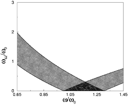
Figure 8: Parameter region in which $k_{-}$ is purely imaginary and $k_{+}>0$ (light shaded area) for $\omega_{p}/\omega_{0}=0.84$. The critical points where curve crossings occur are, from left to right, $\omega$/$\omega_{0}$=$1$ (it separates regions I and II), $\sqrt{1+(\omega_{p}^{2}/2\omega_{0}^{2})}$ (between regions II and III), and $\sqrt{1+(\omega_{p}^{2}/\omega_{0}^{2})}$ (between regions III and IV).

Two other important factors that must be taken into account for the observability and potential application of the polarization filtering are the penetration length of the evanescent wave in the optically active medium, and the transmittance of the surviving mode.

The penetration length is proportional to the inverse of $\rm{Im}(k_{-})$. In practice the medium is not semi-infinite, of course, but the filtering effect may be achieved for a finite medium as long as it extends beyond the penetration length. This should not pose any practical problem according to the scales shown in Fig. 9, where $\omega_{0}/[c\,{\rm{Im}}(k_{-})]$ is shown versus $\omega_{cz}/\omega_{0}$ for $\omega=\omega_{0p}$.

The “transmission probability” $n_{+}|C_{+}|^{2}$ is the ratio between the energy flux of the surviving polarization and the inicident flux. It is showed in Fig. 10 for $\omega_{0}=\omega_{p}$. Up to a significant $25\%$ of transmission may be obtained.

Figure 9: Dimensionless penetration length of the evanescent wave at $\omega=\omega_{0p}$ for with $\omega_{p}/\omega_{0}=1$.

Figure 10: Transmittance of the surviving mode at $\omega=\omega_{0p}$ for $\omega_{p}/\omega_{0}=1$.

Finally, real materials hold multiple resonances but our analysis can be easily generalized by summing over them with appropriate oscillator strenghts factors Fowles .

VI Discussion

In summary, we have shown that the atomic time-dependent Rabi oscillation and its suppression for moving atoms incident on a laser-illuminated region, is analogous to the time-dependent polarization rotation and its suppression for light pulses entering into an optically active medium. The eigenmodes in the laser region depend on Rabi frequency and detuning and in the optically active medium on the susceptibility matrix elements. Since ultrashort femtosecond pulses can be tracked experimentally by interferometric photon scanning tunneling microscopy (PSTM) PSTM , the time dependence of polarization rotation and its suppressions, by averaging, pulse splitting or filtering, can be tested experimentally. These effects may be of interest for the design of an all-optical computer with information encoded, transfered or manipulated using the polarization state; similarly, their atomic counterparts may be relevant in metrology and provide a mechanism for controlled quantum internal state preparation by projection or filtering, i.e., irrespective of the initial state, so that their experimental examination at a light-optics level is both feasible and worthwhile pursuing. The optical analog of atomic state-filtering provides a way to produce polarized light. Whereas the atomic state may be selected by playing with the laser detuning and intensity, the polarization may be selected by a magnetic field.

Appendix A Susceptibility tensor elements

The general expressions for the elements of the ${\bm{\chi}}$ tensor for a homogeneous dielectric in a magnetic field are obtained here from a simple, classical, Lorentz model. Each electron displacement from its equilibrium position ${\bf r}_{e}$ is assumed to satisfy

$$m_{e}\frac{d^{2}{\bf r}_{e}}{dt^{2}}=-e{\bf E}-e\frac{d{\bf r}_{e}}{dt}\times{\bf B}-K{\bf r}_{e}-m_{e}\gamma\frac{d{\bf r}_{e}}{dt}$$ (66)

where $K$ is an elastic force constant that keeps it bound, ${\bf B}$ is a static, external magnetic field, $m_{e}$ the mass of the electron and $\gamma$ a damping constant. (We neglect the small force due to the magnetic field of the optical wave). Assumming that the applied electric field and ${\bf r}_{e}$ vary harmonically as $e^{-i\omega t}$, and using ${\bf{P}}=-Ne{\bf r}_{e}={\bm{\chi}}\epsilon_{0}{\bf E}$ with $N$ the number of electrons per unit volume, a lengthy but straighforward calculation gives, for $\gamma=0$,

$$\chi_{11} = \omega_{p}^{2}\frac{(\omega_{0}^{2}-\omega^{2})^{2}-\omega^{2}\omega_{cx}^{2}}{[(\omega_{0}^{2}-\omega^{2})^{2}-\omega^{2}\omega_{c}^{2}](\omega_{0}^{2}-\omega^{2})}$$ (67)

$$\chi_{12} = \omega_{p}^{2}\frac{\omega[i\omega_{cz}(\omega_{0}^{2}-\omega^{2})-\omega_{cx}\omega_{cy}\omega]}{[(\omega_{0}^{2}-\omega^{2})^{2}-\omega^{2}\omega_{c}^{2}](\omega_{0}^{2}-\omega^{2})}$$

$$\chi_{13} = \omega_{p}^{2}\frac{\omega[-i\omega_{cy}(\omega_{0}^{2}-\omega^{2})-\omega_{cx}\omega_{cz}\omega]}{[(\omega_{0}^{2}-\omega^{2})^{2}-\omega^{2}\omega_{c}^{2}](\omega_{0}^{2}-\omega^{2})}$$

$$\chi_{22} = \omega_{p}^{2}\frac{(\omega_{0}^{2}-\omega^{2})^{2}-\omega^{2}\omega_{cy}^{2}}{[(\omega_{0}^{2}-\omega^{2})^{2}-\omega^{2}\omega_{c}^{2}](\omega_{0}^{2}-\omega^{2})}$$

$$\chi_{23} = \omega_{p}^{2}\frac{\omega[i\omega_{cx}(\omega_{0}^{2}-\omega^{2})-\omega_{cy}\omega_{cz}\omega]}{[(\omega_{0}^{2}-\omega^{2})^{2}-\omega^{2}\omega_{c}^{2}](\omega_{0}^{2}-\omega^{2})}$$

$$\chi_{33} = \omega_{p}^{2}\frac{(\omega_{0}^{2}-\omega^{2})^{2}-\omega^{2}\omega_{cz}^{2}}{[(\omega_{0}^{2}-\omega^{2})^{2}-\omega^{2}\omega_{c}^{2}](\omega_{0}^{2}-\omega^{2})}$$

where

$$\omega_{0} = \sqrt{K/m_{e}},$$ (68)

$$\omega_{c} = eB/m_{e},\;\;\omega_{cu}=eB_{u}/m_{e},\;\;u=x,y,z,$$ (69)

$$\omega_{p} = \left(\frac{Ne^{2}}{m_{e}\epsilon_{0}}\right)^{1/2},$$ (70)

are resonance, cyclotron, and “plasma” frequencies, respectively, and $B=(B_{x}^{2}+B_{y}^{2}+B_{z}^{2})^{1/2}$.

In the hermitian case, i.e., for $\gamma=0$, $\chi_{ij}=\chi_{ji}^{*}$. If $\gamma\neq 0$ the elements in Eq. (67) would have the same form except for the substitution

$$(\omega_{0}^{2}-\omega^{2})\to(\omega_{0}^{2}-\omega^{2}-i\gamma\omega).$$ (71)

The other non-diagonal elements $\chi_{ij}$ can be obtained formally by taking first the complex conjugate of the expressions of the transpose elements $\chi_{ji}$ in Eq. (67) and then making the substitution of Eq. (71).

References

- (1) D. Mugnai and A. Ranfagni, in Time in Quantum Mechanics, ed. by J. G. Muga, R. Sala and I. L. Egusquiza (Springer, Berlin, 2002), Ch. 12.
- (2) A. Steinberg, in Time in Quantum Mechanics, ed. by J. G. Muga, R. Sala and I. L. Egusquiza (Springer, Berlin, 2002), Ch. 11.
- (3) N. F. Ramsey, Molecular Beams (Oxford University Press, New York, 1985).
- (4) S. Haroche, M. Brune and J. M. Raimond, J. Phys. II France 2, 659 (1992).
- (5) J. Baudon, R. Mathevet and J. Robert, J. Phys. B: At. Mol. Opt. Phys. 32, R173 (1999).
- (6) J. A. Damborenea, I. L. Egusquiza, G. C. Hegerfeldt, and J. G. Muga, Phys. Rev. A 66, 052104 (2002).
- (7) B. Navarro, I. L. Egusquiza, J. G. Muga, and G. C. Hegerfeldt, Phys. Rev. A 67, 063819 (2003).
- (8) V. Hannstein, G. C. Hegerfeldt and J. G. Muga, J. Phys. B: At. Mol. Opt. Phys. (2005), in press; quant-ph/0412054.
- (9) M. Büttiker in Time in Quantum Mechanics, ed. by J. G. Muga, R. Sala and I. L. Egusquiza (Springer, Berlin, 2002), Ch. 9.
- (10) R. Sala, D. Alonso, and I. Egusquiza, in Time in Quantum Mechanics, ed. by J. G. Muga, R. Sala and I. L. Egusquiza (Springer, Berlin, 2002), Ch. 8.
- (11) C. Bracher, J. Phys. B: At. Mol. Opt. Phys. 30, 2717 (1997).
- (12) R. Arun and G. S. Agarwal, Phys. Rev. A 64, 065802 (2001).
- (13) V. Buzek, R. Derka, S. Massar, Phys. Rev. Lett. 82, 2297 (1999).
- (14) V. Gasparian, M. Ortuño, J. Ruiz, and E. Cuevas, Phys. Rev. Lett. 75, 2312 (1995).
- (15) Y. Japha, G. Kurizki, Phys. Rev. A 60, 1811 (1999).
- (16) M. Deutsch and J. E. Golub, Phys. Rev. A 53, 434 (1996).
- (17) J. Y. Lee, H. W. Lee, J. W. Hahn, J. Opt. Soc. Am. B 17, 401 (2000).
- (18) V. S. Zaspasskii and G. G. Kozlov, Optics and Spectroscopy 78, 88 (1995). cs and Spectroscopy 78, 88 (1995).
- (19) G. R. Fowles, Introduction to Modern Optics, (Dover, New York. 1975).
- (20) L. Mandel and E. Wolf, Optical Coherence and Quantum Optics (Cambridge, New York, 1995).
- (21) M. Born and E. Wolf, Principles of Optics (Cambridge, New York, 1999, 7th edition).
- (22) H. Gersen, J. P. Korterik, N. F. van Hulst and L. Kuipers, Phys. Rev. E 68, 026604 (2003).