Dynamics of Entanglement for One-Dimensional Spin Systems in an External Time-Dependent Magnetic Field

Abstract

We study the dynamics of entanglement for the XY-model, one-dimensional spin systems coupled through nearest neighbor exchange interaction and subject to an external time-dependent magnetic field. Using the two-site density matrix, we calculate the time-dependent entanglement of formation between nearest neighbor qubits. We investigate the effect of varying the temperature, the anisotropy parameter and the external time-dependent magnetic field on the entanglement. We have found that the entanglement can be localized between nearest neighbor qubits for certain values of the external time-dependent magnetic field. Moreover, as known for the magnetization of this model, the entanglement shows nonergodic behavior, it does not approach its equilibrium value at the infinite time limit.

I introduction

Quantum entanglement is regarded as the resource of quantum information processing with no classical analogdiviccezo ; entg1 ; Nielsen ; gruska . The corresponding investigation is currently a very active area of research vedral ; hill ; Wootters98 ; vidal ; ebr ; blatt due to its potential applications in quantum communication, such as quantum teleportation entg2 ; dik , superdense coding entg3 , quantum key distribution entg4 , telecoloning entg5 and decoherence in quantum computersdiv ; whaley .

Multiparticles systems are the central interest in the field of quantum information, in particular, the quantification of the entanglement contained in quantum states, because the entanglement is the physical resource to perform some of the most important quantum information tasks, like quantum information transfer or quantum computation. Osterloh et.alOsterloh02 connected the theory of critical phenomena with quantum information by exploring the entangling resources of a system close to quantum critical point in a class of one-dimensional magnetic systems.

Recentlyomar , we have demonstrated that for a class of one-dimensional magnetic systems entanglement can be controlled and tuned by varying the anisotropy parameter in the XY Hamiltonian and by introducing impurities into the systems in the equilibrium state. However, offering a potentially ideal protection against environmentally induced decoherence is difficult in information encoding and readout. An important motivation to study the dynamics of entanglement while varying an external magnetic field is to investigate whether it is possible to protect the entanglement from the effects of environment such as an external magnetic field and change of temperature.

Amico et. alAmico04 study the dynamics of entanglement in one-dimensioanl spin systems using Ising-type models. They analyze the time evolution of initial Bell states created in a fully polarized background and on the ground state. They have found that the pairwise entanglement propagates with a velocity proportional to the reduced interaction for all the four Bell states. Moreover, they show that the ”entanglement wave” evolving from a Bell state on the ground state turns out to be very localized in space time.

In this paper, we consider the dynamics of a set of localized spin-1/2 particles coupled through an exchange interaction and subject to an external time-dependent magnetic field. In Sec. II, we introduce the Liouville equation for the density matrix and present the numerical solution of the general XY-model in a lattice with $N$ sites in an external time-dependent magnetic field $h(t)$. In Sec. III, the solutions presented in the previous section are used to compute the magnetization and spin-spin correlation functions. The entanglement of formation is briefly introduced in Sec. IV and expressed in terms of the different spin-spin correlation functions. Finally, Sec. V is devoted to the results and discussions.

II Solution of the time-dependent XY model

In this section, we present the numerical solution of the XY model for a one-dimensional lattice with $N$ sites in an external time-dependent magnetic field $h(t)$. The Hamiltonian for such a chain of interacting spins, with nearest-neighbor interaction only, is given by

$$H=-\frac{J}{2}(1+\gamma)\sum_{i=1}^{N}\sigma_{i}^{x}\sigma_{i+1}^{x}-\frac{J}{2}(1-\gamma)\sum_{i=1}^{N}\sigma_{i}^{y}\sigma_{i+1}^{y}-\sum_{i=1}^{N}h(t)\sigma_{i}^{z}\,,$$ (1)

where $J$ is the coupling constant, $\sigma^{a}$ are the Pauli matrices ($a=x,y,z$), and $\gamma$ is the degree of anisotropy. We set $J=1$ for convenience. The periodic boundary condition is cyclic, namely, $\sigma_{N+1}^{a}=\sigma_{1}^{a}$.

The standard procedure used to solve Eq.(1) is to transform the spin operators into fermionic operatorsLieb ; Barouch70 . Let us define the raising and lowering operators $a_{i}^{+}$, $a_{i}$,

$$a_{i}^{+}=\frac{1}{2}(\sigma_{i}^{x}+i\sigma_{i}^{y}),~{}~{}~{}~{}a_{i}=\frac{1}{2}(\sigma_{i}^{x}-i\sigma_{i}^{y}),$$ (2)

in terms of which the Pauli matrices are given by

$$\sigma_{i}^{x}=a_{i}^{+}+a_{i},~{}~{}~{}~{}\sigma_{i}^{y}=\frac{a_{i}^{+}-a_{i}}{i},~{}~{}~{}~{}\sigma_{i}^{z}=2a_{i}^{+}a_{i}-I.$$ (3)

These operators can be expressed in terms of Fermi operators $b_{i}$, $b_{i}^{+}$

$$a_{i}=exp(-\pi i\sum_{j=1}^{i-1}b_{j}^{+}b_{j})b_{i},~{}~{}~{}~{}a_{i}^{+}=b_{i}^{+}exp(\pi i\sum_{j=1}^{i-1}b_{j}^{+}b_{j}).$$ (4)

Next, we introduce the Fourier transform for a general $h(t)$

$$b_{j}^{+}=\frac{1}{\sqrt{N}}\sum_{p=-N/2}^{N/2}exp(ij\phi_{p})c_{p}^{+}~{},~{}~{}~{}~{}b_{j}=\frac{1}{\sqrt{N}}\sum_{p=-N/2}^{N/2}exp(-ij\phi_{p})c_{p}~{},$$ (5)

where $\phi_{p}=\frac{2\pi p}{N}$. Thus, the Hamiltonian assumes the following form

$$H=\sum_{p=1}^{N/2}{\alpha_{p}(t)[c_{p}^{+}c_{p}+c_{-p}^{+}c_{-p}]+i\delta_{p}[c_{p}^{+}c_{-p}^{+}+c_{p}c_{-p}]+2h(t)}~{}.$$ (6)

where $~{}\alpha_{p}(t)=-2cos\phi_{p}-2h(t)~{}$ and $~{}\delta_{p}=2\gamma sin\phi_{p}~{}$. Since $~{}[\tilde{H}_{p},\tilde{H}_{q}]=0~{}$, we can write Eq. (6) as

$$H=\sum_{p=1}^{N/2}\tilde{H}_{p},$$ (7)

with

$$\tilde{H}_{p}=\alpha_{p}(t)[c_{p}^{+}c_{p}+c_{-p}^{+}c_{-p}]+i\delta_{p}[c_{p}^{+}c_{-p}^{+}+c_{p}c_{-p}]+2h(t)~{}.$$ (8)

This means that the space of $\tilde{H}$ can be decomposed into noninteracting subspaces, each of four dimensions. Using the following basis for the pth subspace:

$$(|0>;c_{p}^{+}c_{-p}^{+}|0>;c_{p}^{+}|0>;c_{-p}^{+}|0>),$$ (9)

we can explicitly obtain

$$\tilde{H}_{p}(t)=\scriptsize{\left(\begin{array}[]{cccc}2h(t)&-i\delta_{p}&0&0\\ i\delta_{p}&-4cos\phi_{p}-2h(t)&0&0\\ 0&0&-2cos\phi_{p}&0{}\\ 0&0&0&-2cos\phi_{p}\end{array}\right)}.$$ (10)

In this paper, the initial condition chosen at $t=0$ is thermal equilibrium of the system, namely, the density matrix of the pth subspace at time $t$ $\rho_{p}(t)$ is given by

$$\rho_{p}(0)=e^{-{\beta}\tilde{H}_{p}(0)},\;\;\;\beta=1/kT$$ (11)

$k$ is the Boltzmann constant. Therefor, using Eq. (10), we obtain

$$\rho_{p}(0)=e^{2{\beta}cos\phi+2{\beta}\Lambda[h(0)]}\scriptsize{\left(\begin{array}[]{cccc}k_{11}^{p}&k_{12}^{p}&0&0\\ k_{21}^{p}&k_{22}^{p}&0&0\\ 0&0&k_{33}^{p}&0{}\\ 0&0&0&k_{44}^{p}\end{array}\right)}.$$ (12)

where

$$\Lambda[h(0)]=\{[cos\phi+h(0)]^{2}+\gamma^{2}sin^{2}\phi\}^{1/2}~{},$$ (13)

and the matrix elements are given by

$$k_{11}^{p}=\frac{\{\Lambda[h(0)]+cos\phi+h(0)\}e^{-4\beta\Lambda[h(0)]}+\{\Lambda[h(0)]-cos\phi-h(0)\}}{2\Lambda[h(0)]}~{},$$ (14)

$$k_{12}^{p}=\frac{i\delta\{1-e^{-4\beta\Lambda[h(0)]}\}}{4\Lambda[h(0)]}~{},$$ (15)

$$k_{21}^{p}=\frac{-i\delta\{1-e^{-4\beta\Lambda[h(0)]}\}}{4\Lambda[h(0)]}~{},$$ (16)

$$k_{22}^{p}=\frac{\{\Lambda[h(0)]-cos\phi-h(0)\}e^{-4\beta\Lambda[h(0)]}+\{\Lambda[h(0)]+cos\phi+h(0)\}}{2\Lambda[h(0)]}~{},$$ (17)

$$k_{33}^{p}=k_{44}^{p}=e^{-2\beta\Lambda[h(0)]}~{}.$$ (18)

Let $U_{p}(t)$ be the time-evolution matrix in the pth subspace, then

$$i\frac{dU_{p}(t)}{dt}=U_{p}(t)\tilde{H}_{p}(t)~{},\;\;\;\hbar=1$$ (19)

Since $\tilde{H}_{p}(t)$ is in a block diagonal form

$$U_{p}(t)=\scriptsize{\left(\begin{array}[]{cccc}U_{11}^{p}&U_{12}^{p}&0&0\\ U_{21}^{p}&U_{22}^{p}&0&0\\ 0&0&U_{33}^{p}&0{}\\ 0&0&0&U_{44}^{p}\end{array}\right)}~{},$$ (20)

where the upper-left block is determined from

$$i\frac{d}{dt}\scriptsize{\left(\begin{array}[]{cc}U_{11}^{p}&U_{12}^{p}\\ U_{21}^{p}&U_{22}^{p}\end{array}\right)}=\scriptsize{\left(\begin{array}[]{cc}U_{11}^{p}&U_{12}^{p}\\ U_{21}^{p}&U_{22}^{p}\end{array}\right)}\scriptsize{\left(\begin{array}[]{cc}2h(t)&-i\delta_{p}\\ i\delta_{p}&-4cos\phi_{p}-2h(t)\end{array}\right)}.$$ (21)

Thus, the Liouville equation of the system which is given by

$$i\frac{d\rho(t)}{dt}=[H(t),\rho(t)]$$ (22)

can be solved exactly because it can be decomposed into uncorrelated subspaces. In the $\emph{p}th$ subspace, the solution of Liouville equation is

$$\rho_{p}(t)=U_{p}(t)\rho_{p}(0)U_{p}(t)^{\dagger}~{}.$$ (23)

In this study the magnetic field will be presented by a step function of the form,

$$h(t)=\left\{\begin{array}[]{ll}a&~{}~{}~{}~{}t\leq 0\\ b&~{}~{}~{}~{}t>0\end{array}\right\}$$

which will allow us to obtain the solution of Eq. (19)

$$U_{p}(t)=e^{2itcos\phi}\scriptsize{\left(\begin{array}[]{cccc}U_{11}^{p}&U_{12}^{p}&0&0\\ U_{21}^{p}&U_{22}^{p}&0&0\\ 0&0&U_{33}^{p}&0{}\\ 0&0&0&U_{44}^{p}\end{array}\right)}~{},$$ (24)

where

$$U_{11}^{p}=\frac{-i(cos\phi+b)sin[2t\Lambda(b)]}{\Lambda(b)}+cos[2t\Lambda(b)]~{},$$ (25)

$$U_{12}^{p}=\frac{-\delta sin[2t\Lambda(b)]}{2\Lambda(b)}~{},$$ (26)

$$U_{21}^{p}=\frac{\delta sin[2t\Lambda(b)]}{2\Lambda(b)}~{},$$ (27)

$$U_{22}^{p}=\frac{i(cos\phi+b)sin[2t\Lambda(b)]}{\Lambda(b)}+cos[2t\Lambda(b)]~{},$$ (28)

$$U_{33}^{p}=U_{44}^{p}=1~{}.$$ (29)

From Eq. (23) we can get

$$\rho_{p}(t)=e^{2{\beta}cos\phi+2{\beta}\Lambda[h(0)]}\scriptsize{\left(\begin{array}[]{cccc}\rho_{11}^{p}&\rho_{12}^{p}&0&0\\ \rho_{21}^{p}&\rho_{22}^{p}&0&0\\ 0&0&\rho_{33}^{p}&0{}\\ 0&0&0&\rho_{44}^{p}\end{array}\right)}~{},$$ (30)

where the matrix elements are given by

$$\rho_{11}^{p}=\frac{\{\delta^{2}(b-a)sin^{2}[2t\Lambda(b)]+\zeta\}e^{-4\beta\Lambda(a)}+\delta^{2}(a-b)sin^{2}[2t\Lambda(b)]+\eta}{4\Lambda^{2}(b)\Lambda(a)}$$ (31)

$$\rho_{12}^{p}=\frac{\delta(1-e^{-4\beta\Lambda(a)})\{\Lambda(b)sin[4t\Lambda(b)](b-a)+i\{\Lambda^{2}(b)+2(a-b)(cos\phi+b)sin^{2}[2t\Lambda(b)]\}\}}{4\Lambda^{2}(b)\Lambda(a)}$$ (32)

$$\rho_{22}^{p}=\frac{\{\delta^{2}(a-b)sin^{2}[2t\Lambda(b)]+\eta\}e^{-4\beta\Lambda(a)}+\delta^{2}(b-a)sin^{2}[2t\Lambda(b)]+\zeta}{4\Lambda^{2}(b)\Lambda(a)}$$ (33)

$$\rho_{21}^{p}=(\rho_{12}^{p})^{*}$$ (34)

$$\rho_{33}^{p}=\rho_{44}^{p}=e^{-2\beta\Lambda(a)}$$ (35)

with

$$\zeta=2\Lambda^{2}(b)(\Lambda(a)+cos\phi+a)$$ (36)

$$\eta=2\Lambda^{2}(b)(\Lambda(a)-cos\phi-a)$$ (37)

III MAGNETIZATION AND SPIN-SPIN CORRELATION FUNCTIONS

The magnetization in the XY model is defined as

$$M=\frac{1}{N}\sum_{j=1}^{N}S_{j}^{z}~{},$$ (38)

which can be written in terms of the operators $c_{p}^{+}$ , $c_{p}^{-}$ as

$$M=\frac{1}{N}\sum_{p=1}^{N/2}M_{p},$$ (39)

where $M_{p}=c_{p}^{+}c_{p}+c_{-p}^{+}c_{-p}-1$ . So we can get the z-direction magnetization

$$M_{z}(t)=\frac{1}{N}\frac{Tr[M\rho]}{Tr[\rho]}=\frac{1}{N}\sum_{p=1}^{N/2}\frac{Tr[M_{p}\rho_{p}(t)]}{Tr[\rho_{p}(0)]}.$$ (40)

Using Eqs. (9),(12) and (30) Eq. (40) gives

$$M_{z}(t)=\frac{1}{4N}\sum_{p=1}^{N/2}\frac{tanh[\beta\Lambda(a)]\{2\delta^{2}(b-a)sin^{2}[2t\Lambda(b)]+4\Lambda^{2}(b)(cos\phi+a)\}}{\Lambda^{2}(b)\Lambda(a)}~{}.$$ (41)

The three instantaneous spin-spin correlation functions are defined as

$$S_{lm}^{x}=<S_{l}^{x}S_{m}^{x}>~{},\;\;S_{lm}^{y}=<S_{l}^{y}S_{m}^{y}>~{},\;\;S_{lm}^{z}=<S_{l}^{z}S_{m}^{z}>$$ (42)

Lieb Schultz and Mattis (LSM) Lieb show that

$$S_{lm}^{x}=\frac{1}{4}<B_{l}A_{l+1}B_{l}...A_{m-1}B_{m-1}A_{m}>~{},$$ (43)

$$S_{lm}^{y}=\frac{1}{4}(-1)^{l-m}<A_{l}B_{l+1}A_{l+1}B_{l+2}...B_{m-1}A_{m-1}B_{m}>~{},$$ (44)

$$S_{lm}^{z}=\frac{1}{4}<A_{l}B_{l}A_{m}B_{m}>~{},$$ (45)

where

$$A_{i}=b_{i}^{+}+b_{i}\;;\;\;\;B_{i}=b_{i}^{+}-b_{i}.$$ (46)

These three correlation functions are given as expectation values of products of fermion operators. Using the Wick Wick50 theorem, the expressions can be expressed as Pfaffians $(pf)$. In particular, we have

$$S_{lm}^{x}=\frac{1}{4}pf\scriptsize{\left(\begin{array}[]{ccccccc}<B_{l}A_{l+1}>&<B_{l}B_{l+1}>&\cdot&\cdot&\cdot&<B_{l}B_{m-1}>&<B_{l}A_{m}>\\ {}\hfil&<A_{l+1}B_{l+1}>&\cdot&\cdot&\cdot&<A_{l+1}B_{m-1}>&<A_{l+1}A_{m}>\\ {}\hfil&{}\hfil&\cdot&\cdot&\cdot&\cdot&\cdot\\ {}\hfil&{}\hfil&{}\hfil&\cdot&\cdot&\cdot&\cdot\\ {}\hfil&{}\hfil&{}\hfil&{}\hfil&\cdot&\cdot&\cdot\\ {}\hfil&{}\hfil&{}\hfil&{}\hfil&{}\hfil&<A_{m-1}B_{m-1}>&<A_{m-1}A_{m}>\\ {}\hfil&{}\hfil&{}\hfil&{}\hfil&{}\hfil&{}\hfil&<B_{m-1}A_{m}>\end{array}\right)}$$ (47)

$$S_{lm}^{y}=\frac{(-1)^{l-m}}{4}pf\scriptsize{\left(\begin{array}[]{ccccccc}<A_{l}B_{l+1}>&<A_{l}A_{l+1}>&\cdot&\cdot&\cdot&<A_{l}A_{m-1}>&<A_{l}B_{m}>\\ {}\hfil&<B_{l+1}A_{l+1}>&\cdot&\cdot&\cdot&<B_{l+1}A_{m-1}>&<B_{l+1}B_{m}>\\ {}\hfil&{}\hfil&\cdot&\cdot&\cdot&\cdot&\cdot\\ {}\hfil&{}\hfil&{}\hfil&\cdot&\cdot&\cdot&\cdot\\ {}\hfil&{}\hfil&{}\hfil&{}\hfil&\cdot&\cdot&\cdot\\ {}\hfil&{}\hfil&{}\hfil&{}\hfil&{}\hfil&<B_{m-1}A_{m-1}>&<B_{m-1}B_{m}>\\ {}\hfil&{}\hfil&{}\hfil&{}\hfil&{}\hfil&{}\hfil&<A_{m-1}B_{m}>\end{array}\right)}$$ (48)

$$S_{lm}^{z}=\frac{1}{4}pf\scriptsize{\left(\begin{array}[]{ccc}<A_{l}B_{l}>&<A_{l}A_{m}>&<A_{l}B_{m}>\\ {}\hfil&<B_{l}A_{m}>&<B_{l}B_{m}>\\ {}\hfil&{}\hfil&<A_{m}B_{m}>\end{array}\right)}$$ (49)

where

$$<B_{l}A_{m}> = \frac{1}{N}\sum_{p=1}^{N/2}\frac{1}{\Lambda^{2}(b)\Lambda(a)[1+e^{-2\beta\Lambda(a)}]^{2}}\{sin(\frac{2{\pi}(m-l)p}{N})\{\Lambda^{2}(b){}$$ (50)

$${}+2(a-b)(cos\phi+b)sin^{2}[2t\Lambda(b)]\}+cos(\frac{2{\pi}(m-l)p}{N}){}$$

$${}\{\delta^{2}(b-a)sin^{2}[2t\Lambda(b)]+2\Lambda^{2}(b)(cos\phi+a)\}[1-e^{-4\beta\Lambda(a)}]\}~{},$$

$$<A_{l}A_{m}>=\frac{1}{N}\sum_{p=1}^{N/2}\{2cos(\frac{2\pi(m-l)p}{N})+\frac{i\delta(a-b)sin(\frac{2\pi(m-l)p}{N})sin[4t\Lambda(b)]tanh(\beta\Lambda(a))}{\Lambda(b)\Lambda(a)}\}~{},$$ (51)

$$<B_{l}B_{m}>=\frac{1}{N}\sum_{p=1}^{N/2}\{-2cos(\frac{2\pi(m-l)p}{N})+\frac{i\delta(a-b)sin(\frac{2\pi(m-l)p}{N})sin[4t\Lambda(b)]tanh(\beta\Lambda(a))}{\Lambda(b)\Lambda(a)}\}~{}.$$ (52)

IV ENTANGLEMENT OF FORMATION

The concept of entanglement of formation is related to the amount of entanglement needed to prepare the state $\rho$, where $\rho$ is the density matrix. It was shown by WoottersWootters98 that

$$E(\rho)=\mathcal{E}(C(\rho)),$$ (53)

where the function $\mathcal{E}$ is given by

$$\mathcal{E}=h(\frac{1+\sqrt{1-C^{2}}}{2}),$$ (54)

where $h(x)=-xlog_{2}x-(1-x)log_{2}(1-x)$ and the concurrence C is defined as

$$C(\rho)=max\{0,~{}\lambda_{1}-\lambda_{2}-\lambda_{3}-\lambda_{4}~{}\}.$$ (55)

For a general state of two qubits, $\lambda_{i}$’s are the eigenvalues, in decreasing order, of the Hermitian matrix

$$R\equiv~{}\sqrt{\sqrt{\rho}~{}\tilde{\rho}~{}\sqrt{\rho}},$$ (56)

where $\rho$ is the density matrix and  $\tilde{\rho}$  is the spin-flipped state defined as

$$\tilde{\rho}=(\sigma_{y}\otimes\sigma_{y})\rho^{*}(\sigma_{y}\otimes\sigma_{y}).$$ (57)

Alternatively, the $\lambda_{i}$’s are the square roots of the eigenvalues of the non-Hermitian $\rho\tilde{\rho}$. Since the density matrix $\rho$ follows from the symmetry properties of the Hamiltonian, the $\rho$ must be real and symmetricalOsterloh02 , plus the global phase flip symmetry of Hamiltonian, which implies that $[\sigma^{z}_{i}\sigma^{z}_{j},\rho]=0$, we obtain

$$\rho={\left(\begin{array}[]{cccc}\rho_{1,1}&0&0&\rho_{1,4}\\ 0&\rho_{2,2}&\rho_{2,3}&0\\ 0&\rho_{2,3}&\rho_{3,3}&0\\ \rho_{1,4}&0&0&\rho_{4,4}\end{array}\right)},\\$$ (58)

with

$$\lambda_{a}=\sqrt{\rho_{1,1}\rho_{4,4}}+|\rho_{1,4}|,~{}\lambda_{b}=\sqrt{\rho_{2,2}\rho_{3,3}}+|\rho_{2,3}|,~{}\lambda_{c}=|\sqrt{\rho_{1,1}\rho_{4,4}}-|\rho_{1,4}||,~{}\lambda_{d}=|\sqrt{\rho_{2,2}\rho_{3,3}}-|\rho_{2,3}|.$$ (59)

Using the definition $<A>=Tr(\rho A)$, we can express all the matrix elements in the density matrix in terms of the different spin-spin correlation functions:

$$\rho_{1,1}=\frac{1}{2}M_{l}^{z}+\frac{1}{2}M_{m}^{z}+S_{lm}^{z}+\frac{1}{4},$$ (60)

$$\rho_{2,2}=\frac{1}{2}M_{l}^{z}-\frac{1}{2}M_{m}^{z}-S_{lm}^{z}+\frac{1}{4},$$ (61)

$$\rho_{3,3}=\frac{1}{2}M_{m}^{z}-\frac{1}{2}M_{l}^{z}-S_{lm}^{z}+\frac{1}{4},$$ (62)

$$\rho_{4,4}=-\frac{1}{2}M_{l}^{z}-\frac{1}{2}M_{m}^{z}+S_{lm}^{z}+\frac{1}{4},$$ (63)

$$\rho_{2,3}=S_{lm}^{x}+S_{lm}^{y},$$ (64)

$$\rho_{1,4}=S_{lm}^{x}-S_{lm}^{y}.$$ (65)

V RESULTS AND DISCUSSIONS

Our goal is to examine the dynamics of entanglement in the presence of varying external magnetic field, temperature and the anisotropy parameter $\gamma$. First we describe the dynamics for the Ising model with $\gamma=1$. For a constant magnetic field, it is convenient to define a dimensionless coupling constant $\lambda=J/h$. This model is known to undergo a quantum phase transition at $\lambda_{c}=1$. The magnetization $<\sigma^{x}>$ is different from zero for $\lambda>1$ and it vanishes at the transitiontobias . However, the magnetization $<\sigma^{z}>$ is different from zero for any value of $\lambda$. At the quantum phase transition the correlation length diverges as $\xi\sim|\lambda-\lambda_{c}|^{-1}$. When $\lambda\rightarrow 0$, the ground state becomes a product of spins pointing in the positive $z$-direction. However, in the limit $\lambda\rightarrow\infty$, the ground state becomes again a product of spins pointing in the positive $x$-direction. In both limits the ground state approaches a product state, thus the entanglement vanishes. When $\lambda=1$, a fundamental transition in the form of the ground state occurs and the system develops a nonzero magnetization $<\sigma^{x}>\neq 0$ which grows as $\lambda$ is increased. The calculations of entanglement show that it rises from zero in the two limits $\lambda\rightarrow 0$ and $\lambda\rightarrow\infty$ to a maximum value near the critical point $\lambda_{c}=1$. Moreover, the range of entanglement, that is the maximum distance between two spins at which the concurrence is different from zero, vanishes unless the two sites are at most next-nearest neighbors.

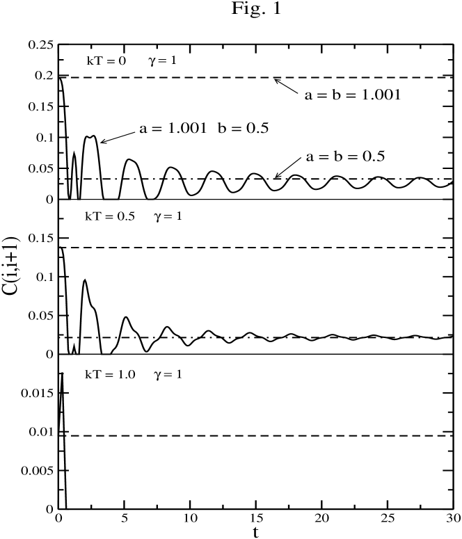
Figure 1: The nearest neighbor concurrence $C(i,i+1)$ for different external magnetic field strengths $a$ and $b$ as a function of time $t$ for $kT=0$ and $kT=0.5$ and $\gamma=1$.

In Fig (1) we show how the nearest neighbor concurrence $C(i,i+1)$ evolves with time when the initial $C(i,i+1)$ close to the maximum. We choose the parameters $a=b=1.001$, $a=b=0.5$ and the step function with $a=1.001$ and $b=0.5$. Thus at $t=0$, $\lambda$ close to one and $C(i,i+1)$ close to maximum. As time evolve, $C(i,i+1)$ oscillate, but it does not reach it is equilibrium value at $t\rightarrow\infty$. Barouch et. al. Barouch70 have shown the nonergodic behavior of the the magnetization for the XY-model. The limit $t\rightarrow\infty$ of the magnetization does not approach its equilibrium value. This phenomenon, the magnetization is not an ergodic observable in this model was discusses earlier by Mazurmazur . The concurrence $C(i,i+1)$ shows a similar behavior, that is nonergodic, since it is related to the magnetization and spin-spin correlation functions. In the lower panel of Fig. (1), we calculate the thermal nearest neighbor concurrence $C(i,i+1)$ as a function of time $t$ for $kT=0.5$ and $kT=1.0$. For this model, the entanglement is nonzero only in a certain region in the $(kt-\lambda)$ planetobias . The entanglement is largest in the vicinity of the critical point $\lambda_{c}=1$ and $kT=0$, this is the quantum critical regime. As expected the concurrence decreases with increasing temperature at $\lambda$ close to one and the oscillations disappeared at $kT=1.0$.

In Fig.(2) we show the nearest neighbor concurrence $C(i,i+1)$ as a function of time $t$ at $kT=0$ and $kT=0.5$ for different parameters of the magnetic field, a step function with an initial field $a=0.5$ and a final field $b=5.0$. For $a=b=0.5$, $\lambda=2>\lambda_{c}=1$ and for $a=b=5.0$, $\lambda=0.2<\lambda_{c}$. One can see that the concurrence starts oscillations when the external magnetic field is applied and reaches a limit when $~{}t\to\infty~{}$, which is again not the equilibrium limit.

In order to investigate the property of concurrence at equilibrium, we calculate the three spin-spin correlation functions as defined in Eq.(43), Eq.(44), Eq.(45) and the magnetization in Eq. (38). Figures (3) and (4) show the behavior of three spin-spin correlation functions and the magnetization as a function of time $t$ at $kT=0$ and $kT=0.5$ respectively. As reported by Barouch et. al.Barouch70 , the magnetization of the Ising model does not approach the equilibrium state limit. Furthermore, we find that the three spin-spin correlation functions do not approach the equilibrium state at $t\to\infty$.

To show the effect of the initial and final external magnetic field strengths on the entanglement with $t\to\infty$, we show in Fig. (5) the nearest neighbor concurrence $C(i,i+1)$ as a function of the parameters $a$ and $b$ at $kT=0$ and $\gamma=1$. For $a<1$ region, the concurrence increases very fast near $b=1$ and reaches a limit $C(i,i+1)\sim 0.125$ when $~{}b\to\infty~{}$. It is surprising that the concurrence will not disappear when $b$ increases with $a<1$. This indicates that the concurrence will not disappear as the final external magnetic field increase at infinite time. It shows that this model is not in agreement with the obvious physical intuition, since we expect that increasing the external magnetic field will destroy the spin-spin correlations functions and make the concurrence vanishes. In our previous calculationsHuang04 , we have found that the concurrence approached a maximum when the external magnetic field is close to the critical point. The concurrence approaches maximum $C(i,i+1)\sim 0.258$ at $(a=1.37,b=1.37)$, and decreases rapidly as $a\neq b$. This indicates that the fluctuation of the external magnetic field near the equilibrium state will rapidly destroy the entanglement. However,in the region where $a>2.0$, the concurrence is close to zero when $b<1.0$ and maximum close to $1$. Moreover, it disappears in the limit of $b\to\infty$.

Recently, it was reported that the nearest neighbor concurrence will decrease as the temperature increases Amico04 at the equilibrium state. It is interesting to investigate the effect of temperature on the concurrence in our model. Fig. (6) shows the nearest neighbor concurrence $C(i,i+1)$ as the parameters $a$ and $b$ varies at $kT=1$. The concurrence in the region where $a<1$ disappears, and the sharp peak shown at $kT=0$ decrease by increasing the temperature. The maximum $C(i,i+1)\sim 0.195$ occurs at $(a=1.76,b=3.0)$.

We now move to consider the dynamics for the anisotropy parameter $\gamma\neq 1$. In Fig.(7) we show the nearest neighbor concurrence $C(i,i+1)$ as a function of time $t$ at $kT=0$ for the same parameters of the magnetic field shown in Fig. (2) for $\gamma=1$. One can see that the concurrence starts oscillations when the external magnetic field is applied and reaches a limit when $~{}t\to\infty~{}$. As for the case $\gamma=1$, this limit is not equivalent to the concurrence for the equilibrium state with $a=b=5.0$. In the lower panel we calculate the thermal nearest neighbor concurrence $C(i,i+1)$ as a function of time $t$ for $kT=0.5$.

Up to now we examined the dynamics of nearest neighbor concurrence $C(i,i+1)$ as a function of the magnetic filed parameters $(a,b)$, the temperature and anisotropy parameter $\gamma$. To describe the dynamics of the next nearest neighbor concurrence $C(i,i+2)$, first we compare in Fig. (8) the behavior of $C(i,i+1)$ and $C(i,i+2)$ as a function of time for same parameters $a=b=1.15$ at $kT=0$ and $\gamma=1$. Although $C(i,i+2)$ shows oscillatory behavior as for $C(i,i+1)$, but the magnitude is very small compared with the $C(i,i+1)$. Moreover, by increasing the temperature $C(i,i+2)$ decreases and vanishes for $kT>0.125$ as shown in Fig. (9). In Fig. (10) we show the dynamics of $C(i,i+2)$ for $\gamma=0.5$ at $kT=0$ and $kT=0.1$. For this case the value of $C(i,i+2)$ is larger than the case with $\gamma=1$ but with similar dynamics. It is interesting to mention that $C(i,i+2)$ is different from zero along the magnetic field parameters $a=b$ as shown in Fig. (11) for $\gamma=1$. The maximum $C(i,i+2)\sim 0.004$ occurs at $(a=1.0,b=1.0)$. For $\gamma=1$ we need to consider only the dynamics of the nearest neighbor $C(i,i+1)$ and next nearest neighbor $C(i,i+2)$ since $C(i,i+3)$ vanishes.

In summary, we have studied the dynamics of entanglement for one-dimensional spin systems in an external magnetic field of a step function form. We observed that the entanglement shows nonergodic behavior. Due to the coherence of the pairwise entanglement with the environment, the change of external magnetic field decreases the nearest and second nearest pairwise entanglement. However, at low temperatures, we have found that there are some regions where there is a decoherence of the entanglement due to the change of the external magnetic field. Finally, we have found that an increase of the temperature in the system will always decrease the pairwise entanglement.

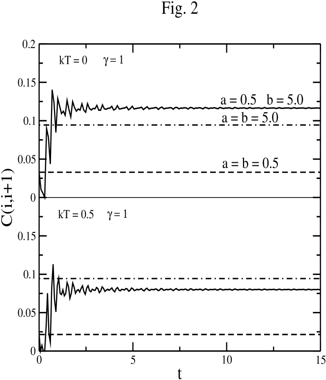
Figure 2: The nearest neighbor concurrence $C(i,i+1)$ for different external magnetic field strengths $a$ and $b$ as a function of time $t$ for $kT=0$ and $kT=0.5$ and $\gamma=1$.

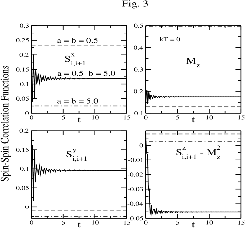
Figure 3: The spin-spin correlation functions and the average magnetization per spin for different external magnetic field strengths $a$ and $b$ as a function of time $t$ at $kT=0$ for $\gamma=1$.

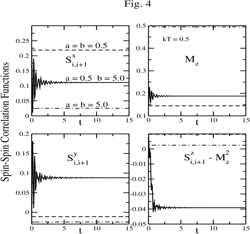
Figure 4: The spin-spin correlation functions and the average magnetization per spin for different external magnetic field strengths $a$ and $b$ as a function of time $t$ at $kT=0.5$ for $\gamma=1$.

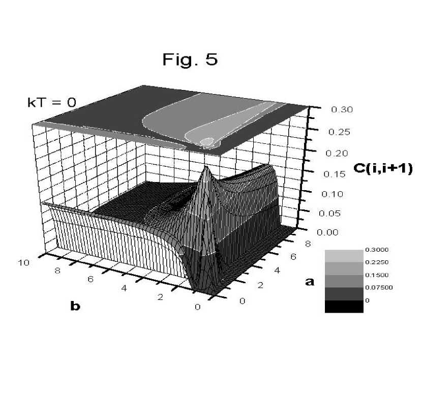
Figure 5: The nearest neighbor concurrence $C(i,i+1)$ as functions of different external magnetic field strengths $a$ and $b$ at time $t\to\infty$ and temperature $kT=0$ for $\gamma=1$.

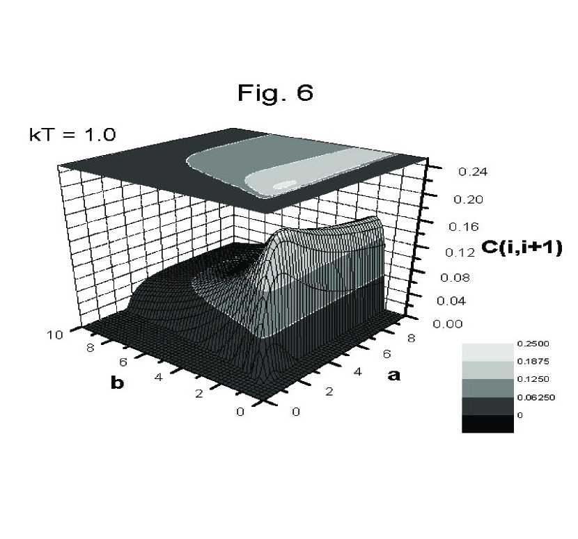
Figure 6: The nearest neighbor concurrence $C(i,i+1)$ as functions of different external magnetic field strengths $a$ and $b$ at time $t\to\infty$ and temperature $kT=1.0$ for $\gamma=1$.

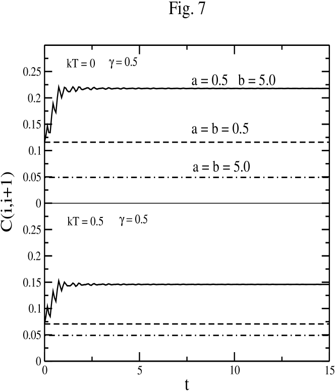
Figure 7: The nearest neighbor concurrence $C(i,i+1)$ for different external magnetic field strengths $a$ and $b$ as a function of time $t$ for $kT=0$ and $kT=0.5$ and $\gamma=0.5$.

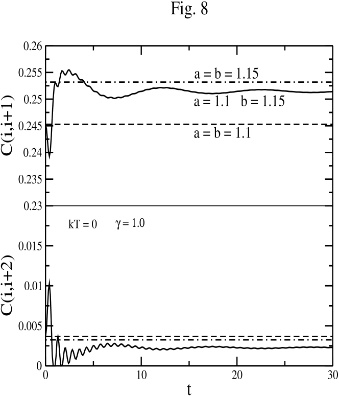
Figure 8: Comparison of the nearest neighbor concurrence $C(i,i+1)$ and the next nearest neighbor concurrence $C(i,i+2)$ for different external magnetic field strengths $a$ and $b$ as a function of time $t$ for $kT=0$ and $\gamma=1$.

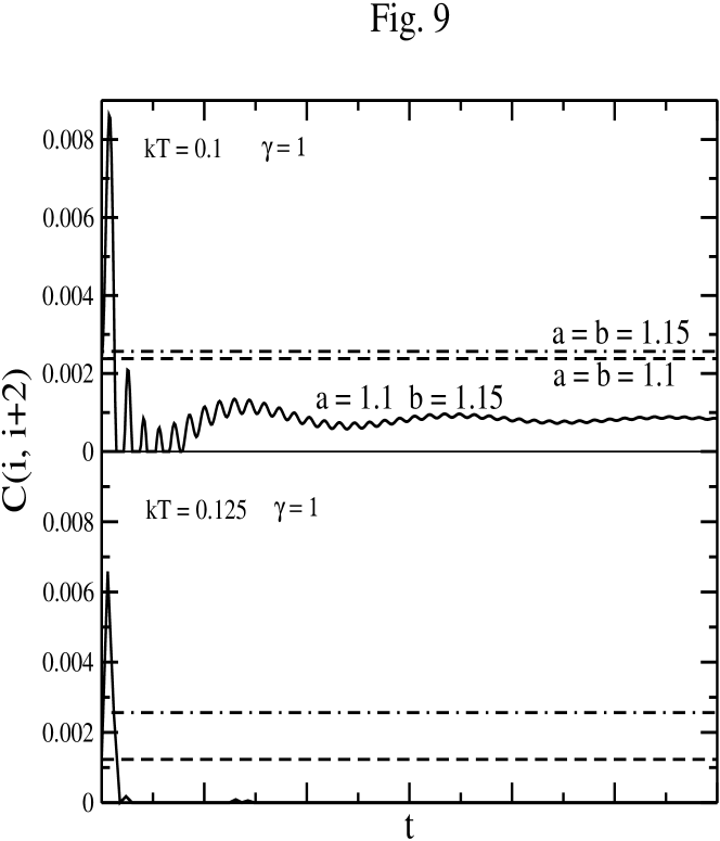
Figure 9: The next nearest neighbor concurrence $C(i,i+2)$ for different external magnetic field strengths $a$ and $b$ as a function of time $t$ for $kT=0.1$ and $kT=0.125$ for the case $\gamma=1$.

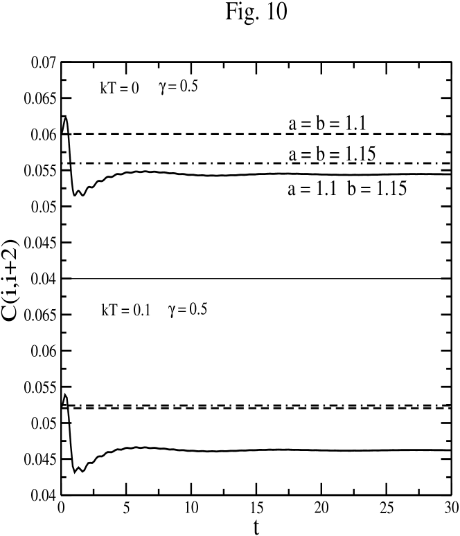
Figure 10: The next nearest neighbor concurrence $C(i,i+2)$ for different external magnetic field strengths $a$ and $b$ as a function of time $t$ for $kT=0$ and $kT=0.1$ for the case $\gamma=0.5$.

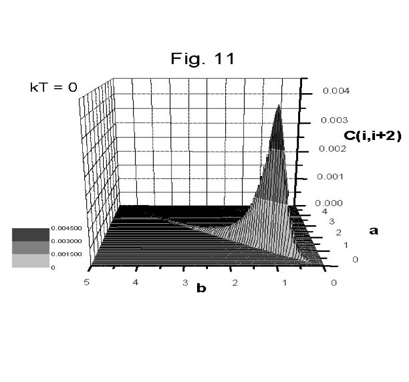
Figure 11: The next nearest neighbor concurrence $C(i,i+2)$ as functions of different external magnetic field strengths $a$ and $b$ at time $t\to\infty$ and temperature $kT=0$ for $\gamma=1$.