An entanglement-area law for general bosonic harmonic lattice systems

Abstract

We demonstrate that the entropy of entanglement and the distillable entanglement of regions with respect to the rest of a general harmonic lattice system in the ground or a thermal state scale at most as the boundary area of the region. This area law is rigorously proven to hold true in non-critical harmonic lattice system of arbitrary spatial dimension, for general finite-ranged harmonic interactions, regions of arbitrary shape and states of nonzero temperature. For nearest-neighbor interactions – corresponding to the Klein-Gordon case – upper and lower bounds to the degree of entanglement can be stated explicitly for arbitrarily shaped regions, generalizing the findings of [Phys. Rev. Lett. 94, 060503 (2005)]. These higher dimensional analogues of the analysis of block entropies in the one-dimensional case show that under general conditions, one can expect an area law for the entanglement in non-critical harmonic many-body systems. The proofs make use of methods from entanglement theory, as well as of results on matrix functions of block banded matrices. Disordered systems are also considered. We moreover construct a class of examples for which the two-point correlation length diverges, yet still an area law can be proven to hold. We finally consider the scaling of classical correlations in a classical harmonic system and relate it to a quantum lattice system with a modified interaction. We briefly comment on a general relationship between criticality and area laws for the entropy of entanglement.

I Introduction

Ground states of quantum systems with many constituents are typically entangled. In a similar manner as one can identify characteristic length scales of correlation functions, quantum correlations are expected to exhibit some general scaling behavior, beyond the details of a fine-grained description. Such characteristic features provide a physical picture that goes beyond the specifics of the underlying microscopic model. A central question of this type is the following: If one distinguishes a certain collection of subsystems, representing some spatial region, of a quantum many-body system in a pure ground state, the state of this part will typically have a positive entropy, reflecting the entanglement between this region and the rest of the system Summers W 85 ; Stelmachovic B 01 ; Osterloh ; NielsenPhase ; Audenaert EPW 02 ; Latorre1 ; Korepin1 ; Fannes . This degree of entanglement is certainly expected to depend on the size and also on the shape of the region. Yet, how does the degree of entanglement specifically depend on the size of the distinguished region? In particular, does it scale as the volume of the interior – which is meant to be the number of degrees of freedom of the interior? Or, potentially as the area of the boundary, i.e., the number of contact points between the interior and the exterior?

This paper provides a detailed answer to the scaling behavior of the entanglement of regions with their exterior in a general setting of harmonic bosonic lattice systems and provides a comprehensive treatment of upper bounds on these quantities. We find that in arbitrary spatial dimensions the degree of entanglement in terms of the von Neumann entropy scales asymptotically as the area of the boundary of the distinguished region. This paper significantly extends the findings of Ref. AreaPRL on harmonic bosonic lattice systems: There, the area-dependence of the geometric entropy has been proven for cubic regions in non-critical harmonic lattice systems of arbitrary dimension with nearest-neighbor interactions, corresponding to discrete versions of Klein-Gordon fields. In this paper we extend our analysis to a general class of finite-ranged harmonic interactions and also take regions of arbitrary shape into account. For thermal Gibbs states, the entropy of a reduction is longer a meaningful measure of entanglement. Instead, an area-dependence for an appropriate mixed-state entanglement measure, the distillable entanglement, is established. Also, an analogous statement holds for classical correlations in classical systems. The area-dependence is even found in certain cases where one can prove the divergence of the two-point correlation length. This demonstrates that this previously conjectured dependence between area and entanglement is valid under surprisingly general conditions.

The presented analysis will make use of methods from the quantitative theory of entanglement in the context of quantum information science Plenio V 98 ; Eisert P 03 ; Plenio V 05 . It has been become clear recently that on questions about scaling of entropies and degrees of entanglement – albeit often posed some time ago – new light can be shed with such methods Summers W 85 ; Stelmachovic B 01 ; Osterloh ; NielsenPhase ; Audenaert EPW 02 ; Latorre1 ; Korepin1 ; Fannes ; Keating ; Cardy ; GraphStates ; Pachos P 04 ; Stabil ; DMRG ; Wolf VC 04 ; Botero R 04 ; Peschel ; Beenakker ; AreaPRL ; Longrange ; Wolf ; Klich ; Orus ; Fine . In this language, quantum correlations are sharply grasped in terms of rates that can be achieved in local physical transformations. To assess quantum correlations using novel powerful tools from quantum information and to relate them to information-theoretical quantities constitutes an exciting perspective.

In the context of quantum field theory, such questions of scaling of entropies and entanglement have a long tradition under the keyword of geometric entropy. In particular, work on the geometric entropy of free Klein-Gordon fields was driven in part by the intriguing suggested connection Callan W 94 to the Bekenstein-Hawking black hole entropy Bekenstein 72 ; Bekenstein 73 ; Bekenstein 04 . In seminal works by Bombelli et al. Bombelli KLS 86 and Srednicki Srednicki 93 the relation between the entropy and the boundary area of the region has been suggested and supplemented with numerical arguments. This connection has been made more specific using a number of different methods. In particular, for half spaces in general and intervals in the one-dimensional case, the problem has been assessed employing methods from conformal field theory, notably Holzhey LW 95 ; Preskill , based on earlier work by Cardy and Peschel CardyPeschel , and by Cardy and Calabrese Cardy .

In one-dimensional non-critical chains, one observes a saturation of the entanglement of a distinguished block, as was proven analytically for harmonic chains AreaPRL ; Audenaert EPW 02 and was later observed for non-critical spin chains numerically Latorre1 and analytically Korepin1 ; Keating ; Cardy . In turn, in critical systems systems, one often – but not always – finds a logarithmically diverging entropy Latorre1 ; Korepin1 ; Keating ; Cardy . In case of a model the continuum limit of which leads to a conformal field theory, the factor of the logarithmically diverging term is related to the central charge of the conformal field theory. The findings of the present paper and of the above-mentioned results motivate further questions concerning the general area-dependence of the degree of entanglement, for example in fermionic systems Wolf ; Klich . In particular, the connection between the geometric entropy fulfilling no area law and the correlated quantum many-body system being critical is not fully understood yet. This is particularly true for the interesting case of more than one-dimensional quantum systems.

This paper is structured as follows. We start, in Section II, with a presentation of the major results of the paper. In Section III we define our notation and recall some basics on harmonic lattice systems. Section IV provides a general framework of upper and lower bounds for entanglement measures, expressed in terms of the spectrum of the Hamiltonian and two-point correlation functions. This analysis is performed both for the case of the ground state as well as for mixed Gibbs states. Of particular interest are Hamiltonians with finite-ranged interactions in Section V. For such Hamiltonians, we first study the behavior of the two-point correlation functions, then the entanglement bounds. In Section VI, discussing the Gibbs state case, we determine temperatures above which there is no entanglement left. A class of examples of Hamiltonians which exhibit a divergent two-point correlation length in their ground state, but an area-dependence of the entanglement is presented in Section IX and expressed in analytical terms. The specific case of Hamiltonians the interaction part of which can be expressed as a square of a banded matrix is discussed in Section VIII. In this case, very explicit expressions for entanglement measures can be found. We then consider, in Section X, the case of classical correlations in classical harmonic systems with arbitrary interaction structure. Interestingly, this case is related to the quantum case for squared interactions in the sense of Section VIII. Finally, we summarize what has been achieved in the present paper, and present a number of open questions in this context.

II Main results

Throughout the whole paper we will consider harmonic subsystems on a $D$-dimensional cubic lattice $C=[1,\dots,n]^{\times D}$. The system thus has $n^{D}$ canonical degrees of freedom. The central question of this work will be: how does the degree of entanglement of a distinguished region $I\subset C$ with the rest $O=C\setminus I$ scale with the size and shape of $I$?

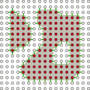
Figure 1: A two-dimensional lattice system $C=[1,...,n]^{\times 2}$ with a distinguished (shaded) region $I$, consisting of $v(I)$ degrees of freedom . Oscillators representing the exterior $O=C\setminus I$ are shown as , whereas pairs belonging to the surface $s(I)$ of the region are marked by lines ().

We define the volume $v(I)$ and surface $s(I)$ of the distinguished region $I$ as

$$v(I)=\sum_{\boldsymbol{i}\in I}1,\;\;\;s(I)=\sum_{\boldsymbol{i}\in O}\sum_{\begin{subarray}{c}\boldsymbol{j}\in I\\ d(\boldsymbol{i},\boldsymbol{j})=1\end{subarray}}1,$$

where

$$d(\boldsymbol{i},\boldsymbol{j})\;\raisebox{0.25832pt}{:}\!\!=\sum_{\delta=1}^{D}|i_{\delta}-j_{\delta}|$$

defines the $1$-norm distance for vectors $\boldsymbol{i}=(i_{1},\dots,i_{D})\in C$ that specify the position of oscillators on the $D$-dimensional lattice. More specifically, $s(I)$ is the number of contact points, that is, the number of pairs of sites of $I$ and $O$ that are immediately adjacent. Note that the distinguished region $I$ may have arbitrary shape and does not have to be contiguous.

For the pure ground state $\varrho$, we will study the entropy of entanglement of $I\subset C$ given by

$$E^{S}_{C,I}=S(\varrho_{I}),$$

where $S=-\operatorname{tr}[\rho\log\rho]$ is the von Neumann entropy of a state $\rho$ and $\varrho_{I}=\operatorname{tr}_{O}[\varrho]$ denotes the reduced state associated with the degrees of freedom of the interior $I$. For the pure ground state, this entropy of entanglement is identical to both the distillable entanglement and the entanglement cost. For pure states, it is indeed the unique asymptotic measure of entanglement. For Gibbs states, in turn, we have to study a mixed-state entanglement measure, as the entropy of a subsystem no longer meaningfully quantifies the degree of entanglement. We will bound the rate at which maximally entangled pairs can be distilled, i.e., the distillable entanglement $E^{D}_{C,I}(T)$. Clearly, $E^{D}_{C,I}(0)=E^{S}_{C,I}$ for zero temperature.

We will subsequently suppress the index $C$ for notational clarity. We derive the following properties of $E^{S}_{I}$ and $E^{D}_{I}(T)$:

• For $D$-dimensional harmonic lattice systems, we derive general upper and lower bounds to $E_{I}^{S}$ for pure ground states and to $E_{I}^{D}(T)$ for Gibbs states with respect to a temperature $T>0$. These bounds are expressed entirely in terms of the potential matrix and stated in Eqs. (8), (9), and (10).

A necessary condition for the following results to hold is that the spectral condition number $\kappa=\lambda_{\text{max}}(V)/\lambda_{\text{min}}(V)$ of the coupling matrix $V$ satisfies $\kappa<c<\infty$ for some $c>0$ independent of $I$ and $O$.

• For nearest-neighbor interactions and the ground state, the entropy of entanglement $E^{S}_{I}$ scales as the surface area $s(I)$ of $I$. More specifically, there exist numbers $c_{1},c_{2}>0$ independent of $O$ and $I$ such that

  $$c_{1}\cdot s(I)<E^{S}_{I}<c_{2}\cdot s(I).$$

  This is stated in Eqs. (12) and (15). Note that the specific case of cubic regions $I=[1,\dots,m]^{\times D}$ has already been proven in the shorter paper Ref. AreaPRL .

• For general finite-ranged harmonic interactions – meaning arbitrary interactions which are strictly zero after a finite distance – the entropy of entanglement $E^{S}_{I}$ of the ground state scales at most linearly with the surface area of $I$: There exists a $c>0$ independent from $O$ and $I$ such that

  $$E^{S}_{I}<c\cdot s(I).$$

  This is expressed in Eq. (12).

• For Gibbs states with respect to a temperature $T>0$ and general finite-ranged interactions the distillable entanglement $E^{D}_{I}(T)$ scales at most linearly with the surface area of $I$, so

  $$E^{D}_{I}(T)<c(T)\cdot s(I),$$

  with $c(T)>0$ being independent of $O$ and $I$, see again Eq. (12), which applies for any temperature. We also determine temperatures above which the entanglement is strictly zero, see Eq. (13).

• We construct a class of Hamiltonians the ground state of which exhibit an infinite two-point correlation length, for which the entropy of entanglement $E^{S}_{I}$ scales provably at most linearly in the boundary area. This is stated in Eq. (20).

• For interactions that are specified by potential matrices $V$ (see Eq. (1)) that can be written as $V=W^{2}$ with $W$ corresponding to a finite-ranged interaction, we determine the entropy of entanglement. This is made specific in particular for $D=1$, see Eq. (19).

• For classical systems of harmonic oscillators with nearest-neighbor interactions prepared in a thermal state, the mutual information

  $$I_{I}(T)=S_{I}(T)+S_{O}(T)-S_{C}(T)$$

  measuring classical correlations scales linearly with the surface area of the region. Here, $S_{I}$, $S_{O}$, and $S_{C}$ are the discrete classical entropies in phase space of the interior, the exterior, and the entire system with respect to an arbitrary coarse graining as defined in Eq. (23), for a classical Gibbs state at temperature $T>0$. The mathematical formulation of the problem is intimately related to case (VI).
  

The remainder of the paper is now concerned with the detailed discussion and rigorous proofs of these statements.

III Harmonic lattice systems – Preliminaries

We consider quantum systems on $D$-dimensional lattices, where each site is associated with a physical system. The starting point is the following Hamiltonian which is quadratic in the canonical coordinates,

$$H=\frac{1}{2}\Bigl{(}\sum_{\boldsymbol{i}}{p}_{\boldsymbol{i}}^{2}+\sum_{\boldsymbol{i},\boldsymbol{j}}{x}_{\boldsymbol{i}}V_{\boldsymbol{i},\boldsymbol{j}}{x}_{\boldsymbol{j}}\Bigr{)}.$$ (1)

The matrix $V$ is the potential matrix. $V_{\boldsymbol{i},\boldsymbol{i}}$ denotes the potential energy contained in the degree of freedom labeled with $\boldsymbol{i}$. For $\boldsymbol{i}\neq\boldsymbol{j}$ the element $V_{\boldsymbol{i},\boldsymbol{j}}$ describes the coupling between the two oscillators at $\boldsymbol{i}$ and $\boldsymbol{j}$. We assume that $V$ is a real symmetric positive matrix. In this paper, we will consider finite-ranged and nearest-neighbor interactions. Furthermore, interactions for which the correlation length diverges are considered.

We will subsequently study properties of both the ground state $\varrho(0)$ as well as of Gibbs states

$$\varrho(T)=\frac{e^{-H/T}}{\operatorname{tr}[e^{-H/T}]}$$

corresponding to some nonzero temperature $T$. Note that we have set the Boltzmann constant $k=1$. The questions we ask are essentially those of the geometric entropy ($T=0$), and those on the distillable entanglement ($T>0$) with respect to a distinguished region $I$ of the lattice $C$. The specific case of nearest-neighbor interactions, considered in Refs. Srednicki 93 ; Audenaert EPW 02 ; AreaPRL ; Botero R 04 corresponds to the one of a discrete version of free Klein-Gordon fields in flat space-time. Here, we consider regions of arbitrary shape and allow for more general interactions.

III.1 Phase space, covariance matrices, and ground states

The system we consider embodies $n^{D}$ canonical degrees of freedom, associated with a phase space $({\mathbbm{R}}^{\times 2\,n^{D}},\sigma)$, where the $(2\,n^{D})\times(2\,n^{D})$-matrix $\sigma$,

$$\sigma\;\raisebox{0.25832pt}{:}\!\!=\left[\begin{array}[]{cc}0_{n^{D}}&{\mathbbm{1}}_{n^{D}}\\ -{\mathbbm{1}}_{n^{D}}&0_{n^{D}}\end{array}\right],$$

specifies the symplectic scalar product, reflecting the canonical commutation relations between the $2\,n^{D}$ canonical coordinates $\boldsymbol{o}=(x_{1},\dots,x_{n^{D}},p_{1},\dots,p_{n^{D}})$ of position and momentum. Instead of considering states we will refer to their moments, considering that both the ground state as well as the Gibbs states are quasi-free (Gaussian) states. The second moments can be collected in the $(2\,n^{D})\times(2\,n^{D})$ real symmetric covariance matrix $\gamma$ (see, e.g., Ref. Eisert P 03 ), defined as

$$\gamma_{j,k}\;\raisebox{0.25832pt}{:}\!\!=2\Re(\operatorname{tr}[\varrho o_{j}o_{k}])=2\Re\langle o_{j}o_{k}\rangle_{\varrho}.$$

Here, it is assumed that the first moments vanish, which does not restrict generality as they can be made to vanish by local unitary displacements that do not affect the entanglement properties.

Following Ref. Audenaert EPW 02 , we find from symplectic diagonalization that for the ground state at zero temperature

$$\gamma_{0}=V^{-1/2}\oplus V^{1/2},$$

i.e., there is no mutual correlation between position and momentum, and the two-point vacuum correlation functions are given by the entries of $V^{-1/2}$ respectively $V^{-1/2}$,

$$G_{\boldsymbol{i},\boldsymbol{j}} \;\raisebox{0.25832pt}{:}\!\!=\langle\text{gs}|x_{\boldsymbol{i}}x_{\boldsymbol{j}}|\text{gs}\rangle=[V^{-1/2}]_{\boldsymbol{i},\boldsymbol{j}},$$ (2)

$$H_{\boldsymbol{i},\boldsymbol{j}} \;\raisebox{0.25832pt}{:}\!\!=\langle\text{gs}|p_{\boldsymbol{i}}p_{\boldsymbol{j}}|\text{gs}\rangle=[V^{1/2}]_{\boldsymbol{i},\boldsymbol{j}}.$$ (3)

Here, $|\text{gs}\rangle$ denotes the state vector of the ground state. For the thermal Gibbs state at finite temperature the covariance matrix takes the form

$$\gamma(T)=\left(V^{-1/2}W(T)\right)\oplus\left(V^{1/2}W(T)\right),$$

where we define

$$W(T)\;\raisebox{0.25832pt}{:}\!\!={\mathbbm{1}}+2(\exp(V^{1/2}/T)-{\mathbbm{1}})^{-1}.$$ (4)

Note that the additional term $W(T)$ is the same for the position as well as for the momentum canonical coordinates. As in the zero temperature case position and momentum are not mutually correlated and $V^{-1/2}W(T)$ ($V^{1/2}W(T)$) are the two-point correlation functions of position (momentum), now with respect to the Gibbs state.

III.2 Measures of entanglement

The entropy of entanglement can be expressed in terms of the symplectic eigenvalues of the covariance matrix corresponding to a reduction. Let the $(2v(I))\times(2v(I))$-matrix $\left.\gamma_{0}\right|_{I}$ denote the covariance matrix associated with the interior $I$; this is the principle submatrix of $\gamma_{0}$ associated with the degrees of freedom of the interior. The symplectic spectrum of $\left.\gamma_{0}\right|_{I}$ is then defined as the spectrum $\mu(B_{I})$ of the matrix

$$B_{I}\;\raisebox{0.25832pt}{:}\!\!=\left(\left.\gamma_{0}\right|_{I}\right)^{1/2}(\mathrm{i}\left.\sigma\right|_{I})\left(\left.\gamma_{0}\right|_{I}\right)^{1/2}.$$

For the situation at hand we find that

$$\left.\gamma_{0}\right|_{I}=\left.V^{-1/2}\right|_{I}\oplus\left.V^{1/2}\right|_{I},$$

where we denote by $V^{\pm 1/2}|_{I}$ the principle submatrix of $V^{\pm 1/2}$ associated with the interior and we index the entries of the submatrix as $[V^{-1/2}]_{\boldsymbol{i},\boldsymbol{j}}$ with vectors $\boldsymbol{i},\boldsymbol{j}\in I$. Given the direct-sum structure of $\gamma_{0}|_{I}$ and counting doubly degenerate eigenvalues only once, we find that the entropy of entanglement can be evaluated as

$$E_{I}^{S}=\sum_{i=1}^{v(I)}\big{[}f\big{(}\frac{\mu_{i}-1}{2}\big{)}-f\big{(}\frac{\mu_{i}+1}{2}\big{)}\big{]},$$ (5)

where $f(x)=-x\log x$, and the $\mu_{i}=\mu_{i}(A_{I})$ are the square roots of the regular eigenvalues $\lambda_{i}=\lambda_{i}(A_{I})$ of the $v(I)\times v(I)$ matrix $A_{I}$,

$$\mu_{i}=\sqrt{\lambda_{i}(A_{I})},\quad A_{I}=\left.V^{-1/2}\right|_{I}\left.V^{1/2}\right|_{I}.$$

This reflects the fact that the entropy of a harmonic system is the sum of the entropies of uncoupled degrees of freedom after symplectic diagonalization.
Using vectors $\boldsymbol{i},\boldsymbol{j}\in I$ to label the entries of $A_{I}$, we find due to $V^{-1/2}V^{1/2}={\mathbbm{1}}$,

$$\begin{split}\left[A_{I}\right]_{\boldsymbol{i},\boldsymbol{j}}&=\left[\left.V^{-1/2}\right|_{I}\left.V^{1/2}\right|_{I}\right]_{\boldsymbol{i},\boldsymbol{j}}\\ &=\delta_{\boldsymbol{i},\boldsymbol{j}}-\sum_{\boldsymbol{k}\in O}\left[V^{-1/2}\right]_{\boldsymbol{i},\boldsymbol{k}}\left[V^{1/2}\right]_{\boldsymbol{k},\boldsymbol{j}}.\end{split}$$ (6)

\psfrag{0}{$0$}\psfrag{Ry30}[lb]{\hskip 5.69046pt$30$}\psfrag{Ry35}[lb]{\hskip 5.69046pt$35$}\psfrag{Ry65}[lb]{\hskip 5.69046pt$65$}\psfrag{Ry70}[lb]{\hskip 5.69046pt$70$}\psfrag{Rx30}{$30$}\psfrag{Rx35}{$35$}\psfrag{Rx65}{$65$}\psfrag{Rx70}{$70$}\psfrag{i}{$i$}\psfrag{j}{$j$}\includegraphics[width=216.81pt]{figures/R_big.eps}

Figure 2: Entries of $R$ in one dimension, $D=1$, for a finite-ranged coupling matrix $V$, $C=[1,...,100]$ and $I=[30,...,35]\cup[65,...,70]$, yielding $s(I)=4$. Bars show $R_{i,j}$, color-encoded surface depicts $\log(R_{i,j})$. All units are arbitrary. Note that the entries decay exponentially away from the boundary of $I$.

This form of $A_{I}={\mathbbm{1}}-R$ hints at an area theorem in the following way (see Fig. 2, where we depict the entries of $R$): if the entries of $V^{\pm 1/2}$ decay fast enough away from the main diagonal, i.e., if the correlation functions decay sufficiently fast, the main contribution to the entropy comes from oscillators inside a layer around the surface of $I$ as for all the others the product $[V^{-1/2}]_{\boldsymbol{i},\boldsymbol{k}}[V^{1/2}]_{\boldsymbol{k},\boldsymbol{j}}$ will be very small (here vectors $\boldsymbol{i},\boldsymbol{j}$ are inside $I$, $\boldsymbol{k}$ outside the region $I$). Thus, the matrix $R$ has an effective rank proportional to $s(I)$, and the number of symplectic eigenvalues contributing to the sum in Eq. (5) is approximately proportional to $s(I)$. Much of the remainder of the paper aims at putting this intuition on rigorous grounds.

For mixed states, such as thermal Gibbs states, the von Neumann entropy no longer represents a meaningful measure of the present quantum correlations, and has to be replaced by concepts such as the distillable entanglement. The distillable entanglement is the rate at which one can asymptotically distill maximally entangled pairs, using only local quantum operations assisted with classical communication. For pure states, it coincides with the entropy of entanglement – the entropy of a reduction – giving an operational interpretation to this quantity Eisert P 03 ; Plenio V 98 ; Plenio V 05 .

From entanglement theory we know that an upper bound for the distillable entanglement is provided by the logarithmic negativity Neg . Note that this is the case even in this infinite-dimensional context for Gaussian states can be immediately verified on the level of second moments and a single-mode description. Moreover, the entropy of entanglement indeed still has the interpretation of a distillable entanglement, albeit the fact that distillation protocols leave the Gaussian setting. This is true as long as one includes an appropriate constraint to the mean energy in the distillation protocol InfContinuous .

The logarithmic negativity Neg is defined as

$$E_{I}^{N}(T)=\|\varrho(T)^{\Gamma}\|_{1},$$

where $\|.\|_{1}$ denotes the trace norm, and $\varrho(T)^{\Gamma}$ is the partial transpose of $\varrho(T)$ with respect to the split $I$ and $O=C\setminus I$. Again following Ref. Audenaert EPW 02 , we find after a number of steps

$$E^{N}_{I}(T)=\sum_{\boldsymbol{i}\in C}\log_{2}\left[\max\left\{1,\lambda_{\boldsymbol{i}}\left(Q\right)\right\}\right],$$ (7)

where $\lambda_{\boldsymbol{i}}(Q)$ labels the $n^{D}$ eigenvalues of $Q$,

$$Q\;\raisebox{0.25832pt}{:}\!\!=P\omega^{-}P\omega^{+},$$

and matrices $\omega^{\pm}(T)$ are defined as

$$\omega^{\pm}(T)\;\raisebox{0.25832pt}{:}\!\!=W(T)^{-1}V^{\pm 1/2},$$

which become $\omega^{\pm}=V^{\pm 1/2}$ for zero temperature following Eq. (4). The diagonal matrix $P$, defined as

$$P_{\boldsymbol{i},\boldsymbol{j}} = \delta_{\boldsymbol{i}\boldsymbol{j}}\left(\delta_{\boldsymbol{i}\in O}-\delta_{\boldsymbol{j}\in I}\right),$$

$$\delta_{\boldsymbol{i}\in S} = \begin{cases}1&\text{if }\boldsymbol{i}\in S\\ 0&\text{otherwise},\end{cases}$$

is the matrix that implements time reversal in the subsystem corresponding to the inner part $I$, reflecting partial transposition $\varrho^{\Gamma}$ on the level of states.

IV Upper and lower bounds

In this section we will derive upper and lower bounds for the entropy of entanglement and the distillable entanglement of the distinguished region $I$ with respect to the rest of the lattice. These bounds only depend on the geometry of the problem, i.e., the region $I$ and on properties of $V$, namely its minimal and maximal eigenvalue, which we define as $a\;\raisebox{0.25832pt}{:}\!\!=\lambda_{\text{min}}(V)$ and $b\;\raisebox{0.25832pt}{:}\!\!=\lambda_{\text{max}}(V)$, respectively, its condition number

$$\kappa\;\raisebox{0.25832pt}{:}\!\!=\frac{b}{a}=\frac{\lambda_{\text{max}}(V)}{\lambda_{\text{min}}(V)},$$

and the entries of $V^{\pm 1/2}$ respectively the two-point correlation functions $G$ and $H$ as in Eqs. (2,3). In later sections these bounds will be made specific for a wide range of interaction matrices $V$.

IV.1 Upper bound

An upper bound for the entropy of entanglement and the distillable entanglement is provided by the logarithmic negativity as in Eq. (7). Utilizing this fact, we derive upper bounds using $l_{1}$-norms Matrix in this section. For brevity and clarity, we will present the case for $T=0$ and finite temperature in a single argument.

A direct calculation shows that the matrix $Q$ is given by

$$Q = \omega^{-}\omega^{+}-2X\omega^{+}$$

$$= W(T)^{-2}-2X\omega^{+},$$

introducing the matrix $X$ with entries

$$X_{\boldsymbol{i},\boldsymbol{j}}\;\raisebox{0.25832pt}{:}\!\!=\omega^{-}_{\boldsymbol{i},\boldsymbol{j}}\left(\delta_{\boldsymbol{i}\in I}\delta_{\boldsymbol{j}\in O}+\delta_{\boldsymbol{i}\in O}\delta_{\boldsymbol{j}\in I}\right).$$

Therefore, we can bound the eigenvalues of $Q$ according to

$$\lambda_{\boldsymbol{i}}(Q) \leq \lambda_{\text{min}}(W(T))^{-2}+\lambda_{\boldsymbol{i}}(-2X\omega^{+})$$

$$\leq \lambda_{\text{min}}(W(T))^{-2}+2\left|\lambda_{\boldsymbol{i}}(X\omega^{+})\right|,$$

where we denote by $\lambda_{\text{min}}(W(T))$ the smallest eigenvalue of $W(T)$ which is given by

$$\lambda_{\text{min}}(W(T))^{-1}=\lambda_{\text{max}}\Big{(}\frac{\mathrm{e}^{V^{1/2}/T}-{\mathbbm{1}}}{\mathrm{e}^{V^{1/2}/T}+{\mathbbm{1}}}\Big{)}=\frac{\mathrm{e}^{\sqrt{b}/T}-1}{\mathrm{e}^{\sqrt{b}/T}+1}.$$

Hence, we can write

$$E_{I}^{N}(T)\leq\sum_{\boldsymbol{i}\in C}\log_{2}\left[\max\left\{1,\lambda_{\text{min}}(W(T))^{-2}+2\left|\lambda_{\boldsymbol{i}}(X\omega^{+})\right|\right\}\right]$$

$$\leq \frac{1}{\ln(2)}\sum_{\boldsymbol{i}\in C}\max\left\{0,\lambda_{\text{min}}(W(T))^{-2}-1+2\left|\lambda_{\boldsymbol{i}}(X\omega^{+})\right|\right\},$$

i.e., for $\lambda_{\text{min}}(W(T))^{-2}+2\max_{\boldsymbol{i}}|\lambda_{\boldsymbol{i}}(X\omega^{+})|<1$, there is no longer any bi-partite entanglement in the system. We will later see that there is a temperature $T_{c}$ above which this happens. But for now, we use the fact that $\lambda_{\text{min}}(W(T))^{-2}\leq 1$ to bound the logarithmic negativity, and relate it to the $l_{1}$ norm $\|.\|_{l_{1}}$ Matrix of $X$. We have $\lambda_{\text{max}}(\omega_{+})=\sqrt{b}/\lambda_{\text{min}}(W(T))$ and therefore

$$E_{I}^{N}(T)\leq\frac{1}{\ln(2)}\sum_{\boldsymbol{i}\in C}2|\lambda_{\boldsymbol{i}}(X\omega^{+})|=\frac{2}{\ln(2)}||X\omega^{+}||_{1}\\ \leq\frac{2\sqrt{b}}{\lambda_{\text{min}}(W(T))\ln(2)}||X||_{1}\leq\frac{2\sqrt{b}}{\lambda_{\text{min}}(W(T))\ln(2)}||X||_{l_{1}}.$$

The $l_{1}$ norm is defined as the sum of the absolute values of all matrix entries. Inserting the definition of $X$, we find

$$\begin{split}\frac{\lambda_{\text{min}}(W(T))\ln(2)}{2\sqrt{b}}E_{I}^{D}&\leq||X||_{l_{1}}=\sum_{\boldsymbol{i},\boldsymbol{j}\in C}\left|X_{\boldsymbol{i},\boldsymbol{j}}\right|\\ &=2\sum_{\begin{subarray}{c}\boldsymbol{j}\in I\\ \boldsymbol{i}\in O\end{subarray}}\left|\omega^{-}_{\boldsymbol{i},\boldsymbol{j}}\right|\end{split}$$ (8)

for finite temperature, and

$$E_{I}^{S}\leq\frac{4\sqrt{b}}{\ln(2)}\sum_{\begin{subarray}{c}\boldsymbol{j}\in I\\ \boldsymbol{i}\in O\end{subarray}}\left|[V^{-1/2}]_{\boldsymbol{i},\boldsymbol{j}}\right|$$ (9)

for zero temperature. These constitute upper bounds on the entropy of entanglement and the distillable entanglement. Both only depend in the distinguished region $I$, the maximum eigenvalue of $V$, and the entries of $V^{-1/2}$, i.e., the two-point correlation function with entries $G_{\boldsymbol{i},\boldsymbol{j}}$. This will be the starting point to derive explicit upper bounds for special types of interaction matrices $V$.

IV.2 Lower bound

To achieve lower bounds for the zero temperature case, we consider the entropy of entanglement directly. Starting from the general expression Eq. (5), we use the fact that the symplectic eigenvalues are never smaller than $1$, i.e., that the eigenvalues of $A_{I}$ are contained in the interval $[1,\alpha_{I}]$, with $\alpha_{I}$ being the maximal eigenvalue of $A_{I}$. Using the pinching inequality Matrix , we find $\alpha_{I}\leq(\lambda_{\text{max}}(V)/\lambda_{\text{min}}(V))^{1/2}=(b/a)^{1/2}=\kappa^{1/2}$. Thus we can bound the entropy of entanglement as follows,

$$E_{I}^{S} \geq \sum_{i=1}^{v(I)}\log[\mu_{i}]=\sum_{i=1}^{v(I)}\frac{\log[\lambda_{i}]}{2}\geq\frac{\log[\alpha_{I}]}{2(\alpha_{I}-1)}\sum_{i=1}^{v(I)}\left(\lambda_{i}-1\right)$$

$$\geq \frac{\log[\sqrt{\kappa}]}{2(\sqrt{\kappa}-1)}\operatorname{tr}\left[A_{I}-{\mathbbm{1}}\right].$$

Using vectors $\boldsymbol{i},\boldsymbol{j}\in I$ to label the entries of the $v(I)\times v(I)$ matrix $A_{I}$, we finally arrive at the lower bound

$$E_{I}^{S} \geq -\frac{\log[\sqrt{\kappa}]}{2(\sqrt{\kappa}-1)}\sum_{\begin{subarray}{c}\boldsymbol{i}\in I\\ \boldsymbol{j}\in O\end{subarray}}\left[V^{-1/2}\right]_{\boldsymbol{i},\boldsymbol{j}}\left[V^{1/2}\right]_{\boldsymbol{j},\boldsymbol{i}}.\;\;\;\;$$ (10)

This lower bound depends only of the geometry of $I$, the spectral condition number $\kappa$ of $V$ and the entries of $V^{\pm 1/2}$, i.e., the two-point correlation functions.

Eq. (10) is difficult to evaluate in general but for special cases of the interaction matrix $V$ it can nevertheless be made specific. In Section VII, for example, we give an explicit expression for the important case of nearest-neighbor interactions. We expect Eq. (10) to be a convenient starting point to derive such lower bounds also for more general cases of $V$.

A lower bound for the finite temperature case is difficult to obtain. Generally speaking, a lower bound to the distillable entanglement (two-way distillable entanglement in our case) is given by the hashing inequality Hashing ,

$$E_{I}^{D}(T)\geq\max\{S(\varrho_{I})-S(\varrho),S(\varrho_{O})-S(\varrho),0\},$$

where $\varrho_{I}=\operatorname{tr}_{O}[\varrho]$ and $\varrho_{O}=\operatorname{tr}_{I}[\rho]$. Yet, naively applied, this inequality will vanish, as generally $S(\varrho_{I})-S(\varrho)<0$ and $S(\varrho_{O})-S(\varrho)<0$: this can be made intuitively clear from the following argument. The above analysis demonstrates that both the interior $I$ and the exterior $O$ can be approximately disentangled with local unitaries up to a layer of the thickness of the two-point correlation length. That is, degrees of freedom associated with $\boldsymbol{i}\in O$ for which $d(\boldsymbol{i},\boldsymbol{j})$ is sufficiently large for every $\boldsymbol{j}\in s(I)$, can to a very good approximation be decoupled and unitarily transformed into a thermal Gibbs state. Each such degree of freedom will therefore contribute a constant number to $S(\varrho)$, such that $S(\varrho_{I})-S(\varrho)<0$ for sufficiently large $n$. Similarly, one can argue to arrive at $S(\varrho_{O})-S(\varrho)<0$. In order to establish a lower bound to the distillable entanglement, however, we may start with any protocol involving only local quantum operations and classical communication, and apply the hashing inequality on the resulting quantum states. This first step can include in particular local filterings. A bound linear in the boundary area is expected to become feasible if one first applies an appropriate unitary both in $I$ and $O$, and then performs a local filtering involving degrees of freedom associated with $\boldsymbol{i}\in I$ and $\boldsymbol{j}\in O$ for which $d(\boldsymbol{i},\boldsymbol{j})=1$. This option will be explored elsewhere.

V Finite-ranged interactions

In this section we will make the upper bound on the entropy of entanglement and the distillable entanglement explicit for symmetric finite-ranged interaction matrices $V$, i.e., matrices for which

$$V_{\boldsymbol{i},\boldsymbol{j}}=0,\;\text{for}\;d(\boldsymbol{i},\boldsymbol{j})>k/2,$$

where $d(\boldsymbol{i},\boldsymbol{j})$ denotes again the $1$-norm distance. Denoting as before the maximum and minimum eigenvalue of $V$ as $a=\lambda_{\text{min}}(V)$ and $b=\lambda_{\text{max}}(V)$ respectively, we require that the spectral condition number $\kappa=b/a$ be strictly less than infinity independent of $C$, i.e., independent of $n$. Note that we do not require any further assumptions on the matrix $V$.

V.1 General upper bounds for finite-ranged interactions

We will make use of a result of Ref. Benzi G 99 concerning the exponential decay of entries of matrix functions. After generalizing this result to matrices $V$ with the properties specified above it enables us to bound the entries of $\omega^{-}$ as follows (see Appendix A)

$$\left|\omega^{-}_{\boldsymbol{i},\boldsymbol{j}}\right|\leq K_{a,b}\,q_{\kappa}^{d(\boldsymbol{i},\boldsymbol{j})},\;\;\;q_{\kappa}=\left(\frac{\kappa-1}{\kappa+1}\right)^{2/k},$$ (11)

and

$$K_{a,b}=\frac{\mathrm{e}^{\eta/T}-1}{\mathrm{e}^{\eta/T}+1}\frac{\kappa+1}{\eta},$$

where

$$\eta\;\raisebox{0.25832pt}{:}\!\!=\left(a\frac{\kappa}{\kappa+1}\right)^{1/2}.$$

For zero temperature we then find

$$K_{a,b}=\frac{\kappa+1}{\sqrt{a}}\left({\frac{\kappa+1}{\kappa}}\right)^{1/2}.$$

This shows that off-diagonal terms of $V^{-1/2}$ decay exponentially, cf. Fig. 3.

\psfrag{0b}[cl]{\color[rgb]{0,0,1}$\scriptstyle 0$}\psfrag{0}[cb]{$\scriptstyle 0$}\psfrag{1}[cc]{\hskip 1.42271pt$\scriptstyle 0$}\psfrag{4}[cc]{\hskip 1.42271pt$\scriptstyle 3$}\psfrag{7}[cc]{\hskip 1.42271pt$\scriptstyle 6$}\psfrag{10}[cc]{\hskip 2.84544pt$\scriptstyle 9$}\psfrag{x3D}{$x_{1}$}\psfrag{y3D}{$x_{2}$}\psfrag{x}[c]{$\scriptstyle x_{1}$}\psfrag{03D}{\hskip 5.69046pt$\scriptstyle 0$}\psfrag{x1}{$\scriptstyle 0$}\psfrag{x4}{$\scriptstyle 3$}\psfrag{x7}{$\scriptstyle 6$}\psfrag{x10}{$\scriptstyle 9$}\psfrag{y1}{$\scriptstyle 0$}\psfrag{y4}{$\scriptstyle 3$}\psfrag{y7}{$\scriptstyle 6$}\psfrag{y10}{$\scriptstyle 9$}\includegraphics[width=216.81pt]{figures/corr2D3D_noshadow.eps}

Figure 3: The entries $[V^{-1/2}]_{\boldsymbol{i},\boldsymbol{j}}$ for a finite-ranged coupling matrix $V$ in two dimensions, $D=2$, $\boldsymbol{j}=\boldsymbol{i}+(x_{1},x_{2})$. Bars show $[V^{-1/2}]_{\boldsymbol{i},\boldsymbol{j}}$ and the color-encoded surface shows $\log([V^{-1/2}]_{\boldsymbol{i},\boldsymbol{j}})$. The inset depicts the same for $x_{1}=x_{2}$. All units are arbitrary. Note the exponential decay away from the main diagonal $\boldsymbol{i}=\boldsymbol{j}$.

Substituting Eqs. (11) into the general result in (8), we find

$$\frac{\lambda_{\text{min}}(W(T))\ln(2)}{4\sqrt{b}K_{a,b}}E_{I}^{N}(T)\leq\sum_{\begin{subarray}{c}\boldsymbol{i}\in I\\ \boldsymbol{j}\in O\end{subarray}}q_{\kappa}^{d(\boldsymbol{i},\boldsymbol{j})}=\sum_{l=1}^{\infty}q_{\kappa}^{l}N_{l},$$

where

$$N_{l}=\sum_{\boldsymbol{j}\in O}\sum_{\begin{subarray}{c}\boldsymbol{i}\in I\\ d(\boldsymbol{i},\boldsymbol{j})=l\end{subarray}}1.$$

Note that $N_{1}=s(I)$ coincides with the definition of the surface area of $I$. We find $N_{l}\leq 2(2l)^{2D-1}s(I)$ (see Appendix C), i.e., we have

$$\sum_{\begin{subarray}{c}\boldsymbol{i}\in I\\ \boldsymbol{j}\in O\end{subarray}}q_{\kappa}^{d(\boldsymbol{i},\boldsymbol{j})}\leq 2^{2D}s(I)\sum_{l=1}^{\infty}q_{\kappa}^{l}l^{2D-1}=\!\!\raisebox{0.25832pt}{:}\;K_{D,\kappa}s(I).$$

Thus we finally arrive at the desired upper bound linear in the surface area of $I$ for both the entropy of entanglement and the distillable entanglement,

$$E_{I}^{N}(T)\leq\frac{4\sqrt{b}K_{a,b}K_{D,\kappa}}{\lambda_{\text{min}}(W(T))\ln(2)}s(I),$$ (12)

which becomes

$$E_{I}^{N}\leq\frac{4(\kappa+1)^{\frac{3}{2}}K_{D,\kappa}}{\ln(2)}s(I)$$

for zero temperature, i.e., these upper bounds depend solely on the maximal and minimal eigenvalue of the interaction matrix $V$ and the surface area of the region $I$. This result demonstrates that indeed, an area-bound of the degree of entanglement holds in generality for bosonic harmonic lattice systems. This shows that the previously expressed intuition can indeed be made rigorous in form of an analytical argument.

V.2 Disordered systems

Notably, the derived results hold also for systems in which the coupling coefficients are not identical, but independent realizations of random variables. If the coefficients $V_{{\boldsymbol{i}},{\boldsymbol{j}}}$ of the real symmetric matrix $V$ are taken from a distribution with a carrier $[x_{0},x_{1}]$, such that the interaction is (i) finite-ranged, and (ii) the carrier is chosen such that

$$\kappa=\frac{\lambda_{\text{max}}(V)}{\lambda_{\text{min}}(V)}<\infty,$$

then the same result holds true. This follows immediately from the considerations in Appendix A, where it is not assumed that the Hamiltonian exhibits translational symmetry. Eq. (12) is thus valid also for disordered harmonic lattice systems.

VI Temperatures above which there is no more entanglement left

In Section IV.1 we found that for $\lambda_{\text{min}}(W(T))^{-2}+2\max_{\boldsymbol{i}}|\lambda_{\boldsymbol{i}}(X\omega^{+})|<1$ there is no entanglement between the regions $I$ and $O$. For finite-range interactions $V$ we found in Section V

$$\max_{\boldsymbol{i}}|\lambda_{\boldsymbol{i}}(X\omega^{+})| \leq \lambda_{\text{min}}(W(T))^{-1}\sqrt{b}||X||_{l_{1}}$$

$$\leq 2\lambda_{\text{min}}(W(T))^{-1}\sqrt{b}K_{a,b}K_{D,\kappa}s(I),$$

i.e., we have

$$\lambda_{\text{min}}(W(T))^{-2}+2\max_{\boldsymbol{i}}|\lambda_{\boldsymbol{i}}(X\omega^{+})|\leq\\ \lambda_{\text{min}}(W(T))^{-2}+4\lambda_{\text{min}}(W(T))^{-1}\sqrt{b}K_{a,b}K_{D,\kappa}s(I).$$

On the right-hand side only $K_{a,b}$ and $\lambda_{\text{min}}(W(T))^{-2}$ depend on the temperature, both are decreasing in $T$ and go to zero as $T$ goes to infinity, i.e.,

$$\lambda_{\text{min}}(W(T))^{-2}+\frac{4\sqrt{b}K_{a,b}K_{D,\kappa}s(I)}{\lambda_{\text{min}}(W(T))}=1$$ (13)

gives an implicit equation for the temperature $T_{c}$ above which there is no bi-partite entanglement left in the system.

VII Nearest-neighbor interactions

In this section we consider nearest-neighbor interactions and periodic boundary conditions in $D$ spatial dimensions, i.e., block-circulant matrices $V$. For $n\rightarrow\infty$ this is a special case of the matrices considered in Section V as boundary conditions become irrelevant in this limit, i.e., the upper bound coincides with the one derived for finite-ranged interactions. For a tighter bound see Appendix B. We will now make use of the circulant structure of $V$ to show that for matrices of this kind it is possible to also derive a lower bound on the entropy of entanglement that it is proportional to the surface area of $I$. We write $M=\operatorname{circ}(\bar{M})$ for the circulant matrix $M$ whose first block column is specified by the tupel of matrices $\bar{M}$. We can then recursively define $V=V_{D}$ via

$$V_{\delta+1}=\operatorname{circ}(V_{\delta},-c{\mathbbm{1}}_{n^{\delta}},0_{n^{\delta}},\dots,0_{n^{\delta}},-c{\mathbbm{1}}_{n^{\delta}}),$$

where $V_{1}=\operatorname{circ}(1,-c,0,\dots,0,-c)$. We choose an energy scale in which $V_{\boldsymbol{i},\boldsymbol{i}}=1$ and we demand $c>0$ plusminus . This circulant structure leads to the following properties of $V$: the eigenvalues of $V$ are given by

$$\lambda_{\boldsymbol{i}}(V)=1-2c\sum_{\delta=1}^{D}\cos\left(2\pi i_{\delta}/n\right),\;\boldsymbol{i}\in C,$$

in particular the maximum eigenvalue is given by $\lambda_{\text{max}}(V)\leq 1+2cD$, where equality holds for $n$ even. The minimum eigenvalue reads $\lambda_{\text{min}}(V)=1-2cD$, i.e., positivity of $V$ demands $c<1/2D$. Note that the assumption that $c<1/2D$ independent of $I$ and $O$ is essential for the argument. If we allow for an $n$-dependence of $c$ as it arises, e.g., in the field-limit where $c=1/(1/n^{2}+2D)$, then in one spatial dimension one will encounter an area law up to a logarithmically divergent correction. This behavior – resembling the behavior of critical spin chains and quadratic fermionic models – will be studied in more detail elsewhere.

Furthermore the circulant nature of $V$ yields the following explicit expressions for the entries of $V^{\pm 1/2}$

$$\left[V^{\pm 1/2}\right]_{\boldsymbol{i},\boldsymbol{j}}=\frac{1}{n^{D}}\sum_{\boldsymbol{k}\in C}\mathrm{e}^{2\pi\mathrm{i}\boldsymbol{k}(\boldsymbol{i}-\boldsymbol{j})/n}\left(\lambda_{\boldsymbol{k}}(V)\right)^{\pm 1/2}.$$ (14)

This reasoning leads to the following properties for $\boldsymbol{i}\neq\boldsymbol{j}$ that are crucial for the present proof (see Appendix B),

$$-[V^{-1/2}]_{\boldsymbol{i},\boldsymbol{j}}[V^{1/2}]_{\boldsymbol{j},\boldsymbol{i}}=\left|[V^{-1/2}]_{\boldsymbol{i},\boldsymbol{j}}[V^{1/2}]_{\boldsymbol{j},\boldsymbol{i}}\right|\\ \geq\left(\frac{c}{2}\right)^{2d(\boldsymbol{i},\boldsymbol{j})}\Big{(}\frac{d(\boldsymbol{i},\boldsymbol{j})!}{(2d(\boldsymbol{i},\boldsymbol{j})-1)\prod_{\delta=1}^{D}|i_{\delta}-j_{\delta}|!}\Big{)}^{2}.$$

Substituting these results into the general lower bound (10) and keeping only terms with $d(\boldsymbol{i},\boldsymbol{j})=1$ immediately yields

$$E^{S}_{I}\geq\frac{\log[\sqrt{\kappa}]c^{2}}{8(\sqrt{\kappa}-1)}s(I),$$ (15)

where

$$\kappa=\frac{1+2cD}{1-2cD}$$

in this case. This generalizes the result of Ref. AreaPRL to regions $I$ of arbitrary shape. We expect that these lower bounds can be generalized to other interactions $V$ and numerical results suggest that these bounds hold quite generally.

VIII Squared interactions

A simple special case is related to a certain kind of interaction: this the one where the interaction matrix $V$ can be written as

$$V=M^{2}$$

with a real symmetric matrix $M$ corresponding to a finite-range interaction. Then, the covariance matrix associated with the interior is nothing but

$$\left.\gamma_{0}\right|_{I}=\left.M^{-1}\right|_{I}\oplus\left.M\right|_{I}.$$ (16)

In this case, the symplectic spectrum can be determined in a fairly straightforward manner. We mention this case also as it appears to be an appropriate toy model as a starting point for studies aiming at assessing the symplectic spectrum of the reduction itself and therefore the spectrum of the reduced density matrix Orus .

We are looking for the spectrum of the $v(I)\times v(I)$ matrix $A_{I}$ as in Eq. (6) which now takes the form (recall that we label the entries of $A_{I}$ by vectors $\boldsymbol{i},\boldsymbol{j}\in I$)

$$\left[A_{I}\right]_{\boldsymbol{i},\boldsymbol{j}}=\delta_{\boldsymbol{i},\boldsymbol{j}}-\sum_{\boldsymbol{k}\in O}[M^{-1}]_{\boldsymbol{i},\boldsymbol{k}}M_{\boldsymbol{k},\boldsymbol{j}}=\delta_{\boldsymbol{i},\boldsymbol{j}}-R_{\boldsymbol{i},\boldsymbol{j}}.$$

It is now the central observation that the number of rows of the matrix $R$ that are nonzero – and therefore also the number of eigenvalues that are nonzero – is proportional to the surface area of $I$, as $M$ is a banded matrix. That is,

$$M_{\boldsymbol{i},\boldsymbol{j}}=0$$

for $d(\boldsymbol{i},\boldsymbol{j})>k/2$, meaning that $R_{\boldsymbol{i},\boldsymbol{j}}=0$ if $d(\boldsymbol{k},\boldsymbol{j})>k/2$ for all $\boldsymbol{k}\in O$. As the eigenvalues of $A_{I}$ are bounded through the pinching inequality by $1$ and $\lambda_{\text{max}}(W)/\lambda_{\text{min}}(W)$, an upper bound linear in the surface area of the interior follows immediately from the fact that the number of eigenvalues entering the sum in Eq. (5) is proportional to $s(I)$. This argument demonstrates that in this simple case, one immediately arrives at bounds that are linear in the number of contact points.

The task of finding the eigenvalues of $A_{I}$ explicitly is now reduced to finding the eigenvalues of the sparse matrix $R$,

$$\mu_{\boldsymbol{i}}(A_{I})=\sqrt{1-\lambda_{\boldsymbol{i}}(R)}.$$

This case is particularly transparent in the one-dimensional case, $D=1$, and for $M$ being a circulant matrix with first row $(1,-c,0,\dots,-c)$ for $0<c<1/2$. The potential matrix $V$ corresponds then to nearest-neighbor interactions, together with next-to-nearest-neighbor interactions. In this one-dimensional setting, we set $I=[1,\dots,m]$. The matrix $R$ then takes the simple form (cf. Fig. 4)

$$R_{i,j} = \sum_{k=m+1}^{n}[M^{-1}]_{i,k}M_{k,j}$$

$$= -c\left([M^{-1}]_{i,m+1}\delta_{j,m}+[M^{-1}]_{i,n}\delta_{j,1}\right).$$

\psfrag{s0b}[cl]{\color[rgb]{0,0,1}$\scriptstyle 0$}\psfrag{s0}[bc]{$\scriptstyle 0$}\psfrag{0}{$\scriptstyle 0$}\psfrag{Rsx1}{$\scriptstyle 1$}\psfrag{Rsx4}{$\scriptstyle 4$}\psfrag{Rsx7}{$\scriptstyle 7$}\psfrag{Rsxa}{$\scriptstyle 11$}\psfrag{Rsxb}{$\scriptstyle 14$}\psfrag{Rsy1}{\hskip 5.69046pt$\scriptstyle 1$}\psfrag{Rsy4}{\hskip 5.69046pt$\scriptstyle 4$}\psfrag{Rsy7}{\hskip 5.69046pt$\scriptstyle 7$}\psfrag{Rsya}{\hskip 5.69046pt$\scriptstyle 11$}\psfrag{Rsyb}{\hskip 5.69046pt$\scriptstyle 14$}\psfrag{q1}[lt]{$\scriptstyle 1$}\psfrag{q4}[lt]{$\scriptstyle 4$}\psfrag{q7}[lt]{$\scriptstyle 7$}\psfrag{ qa}[lt]{$\scriptstyle 11$}\psfrag{ qb}[lt]{$\scriptstyle 14$}\psfrag{i}[cl]{$i$}\psfrag{j}{$j$}\includegraphics[width=216.81pt]{figures/sq_R_noshadow.eps}

Figure 4: Matrix entries of $R$ for the case $D=1$, $C=[1,...,100]$, $I=[1,...,15]$, $V=M^{2}$, where $M$ is a nearest-neighbor circulant matrix. Note that for this particular form of $V$ the entries $R_{i,j}$ are exactly zero for $j\neq 1,m$. This is in contrast to the general form of $R$ depicted in Fig. 2. The inset shows the entries $R_{i,1}$ as bars and $\log(R_{i,1})$ in blue (cf. Eq. (18)).

To find its eigenvalues, we calculate $\det(R-\lambda{\mathbbm{1}})$, which is straightforward for a matrix of this form.

$$\det(R-\lambda{\mathbbm{1}})=-(-\lambda)^{m-2}\det\left(\begin{array}[]{cc}R_{11}-\lambda&R_{1m}\\ R_{m1}&R_{mm}-\lambda\end{array}\right)$$

$$=(-\lambda)^{m-2}(R_{1m}R_{m1}-(R_{11}-\lambda)(R_{mm}-\lambda)),$$

reflecting the fact that $m-2$ eigenvalues are zero, i.e, the number of nonzero eigenvalues is $s(I)=s([1,\dots,m])=2$. We find for the non-vanishing eigenvalues

$$2\lambda_{\pm} = R_{11}+R_{mm}$$

$$\pm \left((R_{11}-R_{mm})^{2}+4R_{1m}R_{m1}\right)^{1/2}.$$

Symmetry of $M^{-1}$ yields

$$\lambda_{\pm}=R_{11}\pm R_{1m}=-c\left([M^{-1}]_{1,n}\pm[M^{-1}]_{m,n}\right).$$

From the circulant structure of $M$ we have

$$[M^{-1}]_{i,j} = \frac{1}{n}\sum_{k=1}^{n}\frac{\mathrm{e}^{2\pi\mathrm{i}k(i-j)/n}}{1-2c\cos(2\pi k/n)}$$

$$= \frac{1}{n}\sum_{k=1}^{n}\frac{\cos(2\pi k(i-j)/n)}{1-2c\cos(2\pi k/n)},$$

i.e., for large $n$ we arrive at

$$[M^{-1}]_{1,n} = \frac{1}{2c\sqrt{1-4c^{2}}}-\frac{1}{2c},$$

$$\ [M^{-1}]_{m,n} = \frac{1}{\sqrt{1-4c^{2}}}\left(\frac{1-\sqrt{1-4c^{2}}}{2c}\right)^{m}.$$ (18)

Note that these expressions are asymptotically independent of $m$ as shown in the inset of Fig. 4. In this limit we finally arrive at

$$\lambda_{\pm}=\frac{1}{2}-\frac{1}{2\sqrt{1-4c^{2}}}.$$ (19)

This expression specifies the symplectic spectrum of the reduction in a closed form.

IX Diverging correlation length and area-law of the entropy

In this section we will analytically demonstrate that there exist Hamiltonians for which the ground state two-point correlation functions diverge whereas the geometric entropy is still bounded by an area-law. In spin systems with a long-range Ising interaction such a behavior has been observed in the one-dimensional case and sketched for higher dimensions Longrange . Here, we present a class of examples of this type valid in arbitrary dimension $D$, for which one can prove the validity of an upper bound linear in the boundary area. Moreover, this set of examples is not restricted to cubic regions. The interaction is here a suitable harmonic long-range interaction. This analysis shows that a divergent two-point correlation function alone is no criterion for a saturating block entropy in the one-dimensional case, and for an area-dependence in higher dimensions.

Consider the matrix $M$ with entries

$$M_{\boldsymbol{i},\boldsymbol{j}} = \frac{1}{d(\boldsymbol{i},\boldsymbol{j})^{\alpha}},$$

$$M_{\boldsymbol{i},\boldsymbol{i}} = 1+\sum_{\begin{subarray}{c}\boldsymbol{j}\in C\\ \boldsymbol{j}\neq\boldsymbol{i}\end{subarray}}\frac{1}{d(\boldsymbol{j},\boldsymbol{i})^{\alpha}}$$

for some $\alpha>0$. Now set $V=M^{-2}$. This choice implies that the correlation function $G_{\boldsymbol{i},\boldsymbol{j}}=[V^{-1/2}]_{\boldsymbol{i},\boldsymbol{j}}$ decays only algebraically. We will show that despite this fact one still has an upper bound linear in the boundary area of $I$ for appropriate values of $\alpha$.

Firstly, we have to make sure that the maximum eigenvalue of $V$ can be bounded from above independent of $n$. From Gershgorin’s theorem (see, e.g., Ref. Matrix ) we know that for every eigenvalue $\lambda(M)$ there exists an ${\boldsymbol{i}}$ such that

$$|\lambda(M)-M_{\boldsymbol{i},\boldsymbol{i}}|\leq\sum_{\begin{subarray}{c}\boldsymbol{j}\in C\\ \boldsymbol{j}\neq\boldsymbol{i}\end{subarray}}M_{\boldsymbol{i},\boldsymbol{j}},$$

i.e.,

$$\lambda_{\text{min}}(M)\geq\min_{i}\Big{[}M_{\boldsymbol{i},\boldsymbol{i}}-\sum_{\begin{subarray}{c}\boldsymbol{j}\in C\\ \boldsymbol{j}\neq\boldsymbol{i}\end{subarray}}M_{\boldsymbol{i},\boldsymbol{j}}\Big{]}=1,$$

and therefore

$$b=\lambda_{\text{max}}(V)=\lambda_{\text{max}}(M^{-2})=\frac{1}{\lambda_{\text{min}}^{2}(W)}\leq 1.$$

Substituting this and the specific form of $M$ into the general expression for the entropy, we obtain

$$\frac{\ln(2)}{4}E_{I}^{S} \leq \sum_{\begin{subarray}{c}\boldsymbol{j}\in I\\ \boldsymbol{i}\in O\end{subarray}}\frac{1}{\left[d(\boldsymbol{i},\boldsymbol{j})\right]^{\alpha}}=\sum_{l=1}^{\infty}\frac{1}{l^{\alpha}}N_{l}$$

$$\leq 2^{2D}s(I)\sum_{l=1}^{\infty}l^{2D-\alpha-1},$$

which converges for $\alpha>2D$ to

$$E_{I}^{S}\leq\frac{2^{2D+2}}{\ln(2)}\zeta(\alpha-2D+1)s(I),$$ (20)

where $\zeta(x)$ is the Riemann zeta function. Note that these bounds are not necessarily tight in the sense that even for smaller values of $\alpha$, such a behavior can be expected. Steps towards tightening these bounds seem particularly feasible in case of cubic regions, where we conjecture that for $\alpha>D$ we arrive at an area-dependence. This analysis shows that for long-range interactions, an area-law in the degree of entanglement can be concomitant with divergent two-point correlation functions.

X An area law for classical correlations

In previous sections we have considered the entanglement between some region and the rest of a lattice of interacting quantum harmonic oscillators with Hamiltonians that are at most quadratic in position and momentum. We have demonstrated that both for the ground state and the thermal state of the entire lattice the quantum correlations, i.e., the amount of entanglement, between the region and the remainder of the lattice is bounded by quantities proportional to their boundary surface area.

This suggests similar questions concerning the classical correlations between a region and the rest of the lattice in the corresponding classical systems when the lattice system as a whole is prepared in a thermal state. In this section we will demonstrate that indeed analogous area laws hold. We will note furthermore that there is a quite striking intimate relation between the classical system with potential matrix $V_{c}$ and the quantum system with a potential matrix $V_{q}=V_{c}^{2}$ in this context.

X.1 Hamiltonian, entropy, and mutual information

For the following considerations we use the classical equivalent of the quantum mechanical Hamiltonian (1), namely again

$$H=\frac{1}{2}\Bigl{(}\sum_{\boldsymbol{i}}{p}_{\boldsymbol{i}}^{2}+\sum_{\boldsymbol{i},\boldsymbol{j}}{x}_{\boldsymbol{i}}V_{\boldsymbol{i},\boldsymbol{j}}{x}_{\boldsymbol{j}}\Bigr{)},$$ (21)

where now $x=(x_{1},\ldots,x_{n^{D}})$ and $p=(p_{1},\ldots,p_{n^{D}})$ are vectors of classical position and momentum variables, respectively, and $V$ denotes again the potential matrix. The state of the classical system is characterized by a phase space density $\varrho=\varrho(\xi)$, a classical probability distribution, where $\xi=(x_{1},\ldots,x_{n^{D}},p_{1},\ldots,p_{n^{D}})$ denotes all the canonical coordinates in phase space. For nonzero temperatures $T>0$ this phase space distribution is given by the Boltzmann distribution

$$\varrho({\xi})=\frac{1}{Z}e^{-\beta H(\xi)}$$ (22)

where $\beta=1/T$ (as before, $k=1$), and

$$Z\;\raisebox{0.25832pt}{:}\!\!=\int d\xi e^{-\beta H(\xi)}.$$

Given this density in phase space we will encounter a familiar ambiguity when defining the entropy of the system. Using the discrete classical entropy Wehrl , we split the phase space into cubic cells each with a volume $h^{2N}$, where $N=k^{D}$ and $h>0$ being an arbitrary constant. From the phase space density we obtain the probability associated with each of these cells which in turn can be used to determine the entropy function of this probability distribution. We will now make use of the multiple indices ${\boldsymbol{i}}=(i_{1},\ldots,i_{N})$ and ${\boldsymbol{j}}=(j_{1},\ldots,j_{N})$, assuming that the cell corresponding to $({\boldsymbol{i}},{\boldsymbol{j}})$ is centered around $x=(hi_{1},\ldots,hi_{N})$ and $p=(hj_{1},\ldots,hj_{N})$. That is, for each degree of the $n^{D}$ degrees of freedom, the phase space is discretized. The contribution of each cell to the discretized probability density is then given by

$$p({\boldsymbol{i}},{\boldsymbol{j}})=\int_{\text{Cell}}d\xi\varrho(\xi)\,.$$

As usual, the discrete classical entropy is then defined as the corresponding Shannon entropy

$$S_{C}(h)\;\raisebox{0.25832pt}{:}\!\!=-\sum_{{\boldsymbol{i}},{\boldsymbol{j}}}p({\boldsymbol{i}},{\boldsymbol{j}})\log p({\boldsymbol{i}},{\boldsymbol{j}})$$ (23)

We will denote the discrete classical entropy with respect to the degrees of freedom of the interior with $S_{I}(h)$, the entropy of the exterior with $S_{O}(h)$.

The value for the entropy will depend on the choice of $h$ and in the limit $h\rightarrow 0$ this entropy definition will diverge due to a term proportional to $-\log(h^{2N})$. In classical statistical mechanics this problem is avoided with the help of the third law of thermodynamics. The entropy itself is however not the quantity that we wish to compute but rather the mutual information $I_{I}$ between the interior $I$ and the rest of a lattice, denoted as before by $O$. This classical mutual information meaningfully quantifies the classical correlations between the inner and the outer. In that case we find that the limit $h\rightarrow 0$ exists and that the mutual information $I$ can be defined as

$$I_{I}\;\raisebox{0.25832pt}{:}\!\!=\lim_{h\rightarrow 0}\left(S_{I}(h)+S_{O}(h)-S_{C}(h)\right).$$

Following these preparations we are now in a position to determine the mutual information between a region and the rest of the lattice explicitly when the lattice as a whole is in a thermal state.

X.2 Evaluation of the mutual information

For the evaluation of the mutual information we need to determine the entropy of the total lattice $C$, as well as the entropy determined by the reduced densities describing the two regions $I$ and $O$. To this end we carry out the partial summation over all degrees of freedom of region $O$ in order to find the reduced phase space density $\varrho_{I}$ describing region $I$ only. Employing the Schur complement we find that the reduced density $\varrho_{I}$ is described by the Boltzmann distribution corresponding to the same temperature and the Hamiltonian

$$H_{I}=\frac{1}{2}\left(\sum_{\boldsymbol{i,j}\in I}x_{\boldsymbol{i}}[(\left.V\right|_{I})^{-1}]_{\boldsymbol{i},\boldsymbol{j}}x_{\boldsymbol{j}}+\sum_{\boldsymbol{i}\in I}p_{\boldsymbol{i}}^{2}\right)$$ (24)

An analogous result holds for the reduced phase space density of region $O$.

For a thermal phase space distribution Eq. (22) corresponding to a classical Hamiltonian function of the form Eq. (21) we can compute the entropy straightforwardly, to find

$$S_{A}=-\frac{1}{2}\log\det\left(\left.V\right|_{A}\right)^{-1}+v(A)\log\frac{2\pi}{\beta}+v(A)$$

$A\in\{I,O,C\}$, which increases with temperature as expected. For the mutual information we find

$$I_{I}=\frac{1}{2}\log\frac{\det\left.V\right|_{I}\det\left.V\right|_{O}}{\det V},$$

which is, perhaps surprisingly, independent of temperature. Using Jacobi’s determinant identity

$$\det\left.V\right|_{O}\det V^{-1}=\det\left.V^{-1}\right|_{I}$$

this expression can be rewritten as

$$I_{I}=\frac{1}{2}\log\det\left[\left.V\right|_{I}\left.V^{-1}\right|_{I}\right]=\frac{1}{2}\log\det\left[{\mathbbm{1}}-R\right].$$

It is now advantageous to notice the close connection of this expression, in particular of the matrix $R$

$$R_{\boldsymbol{i},\boldsymbol{j}}=\sum_{\boldsymbol{k}\in O}[V^{-1}]_{\boldsymbol{i},\boldsymbol{k}}V_{\boldsymbol{k},\boldsymbol{j}}$$

with those that arise in the quantum mechanical problem that we have treated previously in Section VIII. Indeed, the classical problem for a system with potential matrix $V_{\text{c}}$ is related to the quantum mechanical system with the squared potential matrix $V_{\text{q}}=V_{\text{c}}^{2}$. This formal similarity arises because in Section VIII we have shown that for a lattice of quantum harmonic oscillators with potential matrix $V_{\text{q}}=V_{\text{c}}^{2}$ in its ground state the symplectic eigenvalues of the covariance matrix describing region I alone are exactly the standard eigenvalues of the matrix $({\mathbbm{1}}-R)^{1/2}$. The properties of these eigenvalues have already been discussed in detail in Section VIII. This allows us now straightforwardly to establish the area theorem for the mutual information in a classical system employing the result for the corresponding quantum system.

This establishes in particular that the classical correlations as measured by the mutual information $I_{C,I}$ between the distinguished region $I$ and the rest of the lattice $O=C\setminus I$ satisfy

$$c_{1}^{\prime}\cdot s(I)\leq I_{I}(T)\leq c_{2}^{\prime}\cdot s(I)$$

for large $v(I)$ and appropriate constants $c^{\prime}_{1,2}>0$ independent of $O$ and $I$. (Compare also the assessment of the thermodynamical entropy of parts of classical fluids in Ref. Callaway .) In summary we have seen that the area-dependence of correlations is not restricted to quantum systems, as long as one replaces the notion of entanglement – representing quantum correlations – by the notion of classical correlations in a classical system.

XI Summary and outlook

In this paper, we have considered the question of the area-dependence of the geometric entropy and the distillable entanglement in general bosonic harmonic lattice systems of arbitrary dimension. The question was the general scaling behavior of these measures of entanglement with the size of a distinguished region of a lattice. Such an analysis generalizes assessments of block entropies in the one-dimensional case. Using methods from entanglement theory, we established bounds that allow for a conclusion that may be expressed in a nutshell as: in surprising generality, we find that the degree of entanglement scales at most linearly in the boundary area of the distinguished region. This analysis shows that the intuition that both the interior and the exterior can be approximately disentangled up to a layer of the thickness of the two-point correlation length by appropriate local unitaries carries quite far indeed.

For cubic regions $I=[1,...,m]^{\times D}$ the area law can be formulated as

$$E^{D}_{I}=\Theta(m^{D-1}),$$ (25)

where $\Theta$ is the Landau theta.

Such area-laws are expected to have an immediate implication on the accuracy to which ground states can be approximated with matrix-product states and higher dimensional analogues in classical simulations of the ground states of quantum many-body systems DMRG . After all, the failure of DMRG algorithms close to critical points can be related to the logarithmic divergence of the block entropy in the one-dimensional case.

The findings of the present paper raise a number of interesting questions. Notably, in general quantum many-body systems on a lattice (fermionic or bosonic), what are necessary and sufficient conditions for an area-law in the above sense to hold? Clearly, as we have seen above, the divergence of two-point correlation functions alone is not in one-to-one correspondence with an area law. It would be interesting to consider and possibly decide the conjecture that a one-to-one relationship between a system being critical and not satisfying a law of the form as in Eq. (25) holds if one (i) restricts attention to systems in arbitrary dimension with nearest-neighbor interactions, and (ii) grasps criticality in terms of two-point correlation functions with algebraic decay, concomitant with a vanishing energy gap. Note that the latter two criteria of criticality have not been rigorously related to each other yet and may indeed not be simultaneously satisfied in lattice systems. The general relationship is still awaiting rigorous clarification.

As steps towards such an understanding of a relationship between criticality and properties of ground state entanglement in more than one-dimensional fermionic and bosonic systems, it seems very interesting to study models different from the ones considered in this paper. For example, complementing our bosonic analysis, area-laws in fermionic critical systems have been addressed Wolf ; Klich , where logarithmic corrections have been found also in higher-dimensional settings. Other settings in the bosonic case, corresponding to field theories beyond this quasi-free setting, are also still not clarified. In particular, the scaling behavior of the geometric entropy in general bosonic theories in higher dimensions is far from clear. Then, the case of finite-size effects in harmonic lattice systems where the correlation length is larger than the full system, resembling the critical case, will be presented elsewhere. In less generality, it seems also feasible to identify the prefactors of the leading and next-to-leading order terms in an area-law of the geometric entropy. It is the hope that the present work can contribute to an understanding of genuine quantum correlations in quantum many-body systems and inspire such further considerations.

XII Acknowledgments

We would like to thank C. H. Bennett, H. J. Briegel, J. I. Cirac, W. Dür, M. Fleischhauer, B. Reznik, T. Rudolph, N. Schuch, R. G. Unanyan, R. F. Werner, and M. M. Wolf for discussions. This work has been supported by the EPSRC QIP-IRC (GR/S82176/0), the EU Thematic Network QUPRODIS (IST-2002-38877), the DFG (SPP 1078 and SPP 1116), The Leverhulme Trust (F/07 058/U) and the European Research Councils (EURYI).

Appendix A Exponential decay of entries of matrix functions

The result concerning the exponential decay of entries of matrix functions of Ref. Benzi G 99 relies on the fact that the $p$-th power $A^{p}$ of a $k$-banded matrix $A=(A_{i,j})$ is $pk$-banded, i.e., $[A^{p}]_{i,j}=0$ for $|i-j|>pk/2$ for a matrix $A$ with $A_{i,j}=0$ for $|i-j|>k/2$. For the purposes of the present paper, we will need a generalization of the result of Ref. Benzi G 99 to block banded matrices. We refer to $V=(V_{\boldsymbol{i},\boldsymbol{j}})$ as being $k$-banded, if $V_{\boldsymbol{i},\boldsymbol{j}}=0$ for $d(\boldsymbol{i},\boldsymbol{j})>k/2$. It can be proven by induction over $p$ that the $p$-th power of $V$ is $pk$ banded in this sense. This enables us to formulate the general form of Ref. Benzi G 99 as follows.

Let $V=(V_{\boldsymbol{i},\boldsymbol{j}})$ be a $k$-banded symmetric matrix, i.e., $V_{\boldsymbol{i},\boldsymbol{j}}=0$ for $\sum_{\delta}|i_{\delta}-j_{\delta}|>k/2$. Define $a=\lambda_{\text{min}}(V)$, $b=\lambda_{\text{max}}(V)$, $\kappa=b/a$,

$$\psi:{\mathbbm{C}}\rightarrow{\mathbbm{C}},\;\;\;\psi(z)=\frac{(b-a)z+a+b}{2},$$

and $\varepsilon_{\chi}$ as an ellipse with foci in $-1$ and $1$ and half axes $\alpha$, $\beta$, $\chi=\alpha+\beta$.
Now let $f:{\mathbbm{C}}\rightarrow{\mathbbm{C}}$ be such that $f\circ\psi$ is analytic in the interior of the ellipse $\varepsilon_{\chi}$, $\chi>1$, and continuous on $\varepsilon_{\chi}$. Furthermore suppose $(f\circ\psi)(z)\in{\mathbbm{R}}$ for $z\in{\mathbbm{R}}$. Then there exist constants $K$ and $q$, $0\leq K$, $0\leq q\leq 1$ such that

$$\left|[f(V)]_{\boldsymbol{i},\boldsymbol{j}}\right|\leq Kq^{\sum_{\delta=1}^{D}|i_{\delta}-j_{\delta}|},$$

where

$$K=\max\left\{\max_{\boldsymbol{i}}\left|\lambda_{\boldsymbol{i}}(f(V))\right|,\frac{2\chi M(\chi)}{\chi-1}\right\},$$

$$q=\left(\frac{1}{\chi}\right)^{2/k},\quad M(\chi)=\max_{z\in\varepsilon_{\chi}}|(f\circ\psi)(z)|.$$

To bound the entries of $\omega^{-}$, we apply the above theorem to the function

$$\omega^{-}(z)=\frac{\mathrm{e}^{\sqrt{z}/T}-1}{\mathrm{e}^{\sqrt{z}/T}+1}z^{-\frac{1}{2}}.$$

For $1<\chi<(\sqrt{\kappa}+1)^{2}/(\kappa-1)$, we have that $\omega^{-}\circ\psi$ is analytic in the interior of the ellipse $\varepsilon_{\chi}$ and continuous on $\varepsilon_{\chi}$, i.e., $\omega^{-}$ satisfy the assumptions of the above theorem. To make $K$ and $q$ specific, we choose

$$\frac{(\sqrt{\kappa}+1)^{2}}{\kappa-1}>\chi\;\raisebox{0.25832pt}{:}\!\!=\frac{\kappa+1}{\kappa-1}>1,$$

which yields

$$q_{\kappa}=\left(\frac{\kappa-1}{\kappa+1}\right)^{2/k},\quad K_{a,b}=\frac{\mathrm{e}^{\eta/T}-1}{\mathrm{e}^{\eta/T}+1}\frac{\kappa+1}{\eta}$$

where

$$\eta=\left(a\frac{\kappa}{\kappa+1}\right)^{1/2},$$

and for zero temperature $K_{a,b}$ reduces to

$$K_{a,b}=\frac{\kappa+1}{\eta}.$$

These findings explicitly relate the spectral properties of the Hamiltonian to the two-point correlation functions.

Appendix B Entries of the correlation matrix for the nearest-neighbor case

In this appendix, we make the evaluation of the entries of $V^{1/2}$ and $V^{-1/2}$ of the important case of nearest-neighbor interactions specific. The power series expansion of the square root is given by

$$\left(1-x\right)^{\pm\frac{1}{2}}=1\mp\sum_{k=1}^{\infty}a^{\pm}_{k}x^{k},\quad a^{-}_{k}=\prod_{l=1}^{k}\frac{2l-1}{2l},$$

$$a^{-}_{k}\geq\frac{a^{-}_{k}}{2k-1}=a^{+}_{k}\geq\frac{1}{2^{k}(2k-1)},$$

which is valid for $|x|<1$, i.e., the positivity constraint $0<c<1/2D$ allows us to write

$$(\lambda_{\boldsymbol{k}}(V))^{\pm\frac{1}{2}} = 1\mp\sum_{l=1}^{\infty}a^{\pm}_{l}\Big{(}2c\sum_{\delta=1}^{D}\cos\big{(}\frac{2\pi k_{\delta}}{n}\big{)}\Big{)}^{l}$$

$$= 1\mp\sum_{l=1}^{\infty}a^{\pm}_{l}c^{l}\Big{(}\sum_{\delta=1}^{D}\mathrm{e}^{\frac{2\pi\mathrm{i}k_{\delta}}{n}}+\mathrm{e}^{-\frac{2\pi\mathrm{i}k_{\delta}}{n}}\Big{)}^{l}.$$

Using the multinomial theorem, we have

$$\Big{(}\sum_{\delta=1}^{D}\mathrm{e}^{\frac{2\pi\mathrm{i}k_{\delta}}{n}}+\mathrm{e}^{-\frac{2\pi\mathrm{i}k_{\delta}}{n}}\Big{)}^{l}=\sum l!\prod_{\delta=1}^{D}\frac{\big{(}\mathrm{e}^{\frac{2\pi\mathrm{i}k_{\delta}}{n}}+\mathrm{e}^{-\frac{2\pi\mathrm{i}k_{\delta}}{n}}\big{)}^{n_{\delta}}}{n_{\delta}!},$$

where the sum runs over all $n_{\delta}$ with $\sum_{\delta}n_{\delta}=l$. Now, applying the binomial theorem

$$\big{(}\mathrm{e}^{\frac{2\pi\mathrm{i}k_{\delta}}{n}}+\mathrm{e}^{-\frac{2\pi\mathrm{i}k_{\delta}}{n}}\big{)}^{n_{\delta}}=\sum_{r=o}^{n_{\delta}}\binom{n_{\delta}}{r}\mathrm{e}^{\frac{2\pi\mathrm{i}k_{\delta}(n_{\delta}-2r)}{n}}.$$

Substituting all the above into Eq. (14), we find

$$[V^{\pm 1/2}]_{\boldsymbol{i},\boldsymbol{j}}=\delta_{\boldsymbol{i},\boldsymbol{j}}\mp\sum_{l=1}^{\infty}a_{l}^{\pm}c^{l}\sum l!\prod_{\delta=1}^{D}f(d_{\delta},n_{\delta}),$$

where $d_{\delta}=i_{\delta}-j_{\delta}$ and

$$f(d_{\delta},n_{\delta})=\sum_{r=0}^{n_{\delta}}\frac{1}{(n_{\delta}-r)!r!}\sum_{k=1}^{n}\frac{\mathrm{e}^{2\pi\mathrm{i}k(d_{\delta}+n_{\delta}-2r)/n}}{n}.$$

To the sum over $r$ only terms with $d_{\delta}+n_{\delta}-2r=zn$ for some $z\in{\mathbbm{Z}}$ contribute. We thus arrive at the following expression for the entries of $V^{\pm 1/2}$

$$[V^{\pm 1/2}]_{\boldsymbol{i},\boldsymbol{j}}=\\ \delta_{\boldsymbol{i},\boldsymbol{j}}\mp\sum_{l=1}^{\infty}a_{l}^{\pm}c^{l}\!\!\!\!\sum_{\sum_{\delta}n_{\delta}=l}\!\!\!l!\prod_{\delta=1}^{D}\!\!\sum_{\begin{subarray}{c}r=0\\ d_{\delta}+n_{\delta}-2r=zn\end{subarray}}^{n_{\delta}}\!\!\!\!\!\!\!\!\!\!\!\!\!\frac{1}{(n_{\delta}-r)!r!},$$

i.e., for nearest-neighbor interactions the product $-[V^{-1/2}]_{\boldsymbol{i},\boldsymbol{j}}[V^{+1/2}]_{\boldsymbol{i},\boldsymbol{j}}$ is always positive for $\boldsymbol{i}\neq\boldsymbol{j}$. This does not hold in general and makes it difficult to obtain explicit bounds on the entries of $V^{\pm 1/2}$ for more general interactions $V$. To obtain a lower bound we keep only the term $l=d(\boldsymbol{i},\boldsymbol{j})$ and $n_{\delta}=|d_{\delta}|$. The restriction on $r$ is then fulfilled for $r=0$ ($r=|d_{\delta}|$) if $d_{\delta}<0$ ($d_{\delta}>0$), yielding

$$|[V^{\pm 1/2}]_{\boldsymbol{i},\boldsymbol{j}}| \geq a_{d(\boldsymbol{i},\boldsymbol{j})}^{\pm}c^{d(\boldsymbol{i},\boldsymbol{j})}\frac{d(\boldsymbol{i},\boldsymbol{j})!}{\prod_{\delta=1}^{D}|i_{\delta}-j_{\delta}|!}$$

$$\geq \left(\frac{c}{2}\right)^{d(\boldsymbol{i},\boldsymbol{j})}\frac{d(\boldsymbol{i},\boldsymbol{j})!}{(2d(\boldsymbol{i},\boldsymbol{j})-1)\prod_{\delta=1}^{D}|i_{\delta}-j_{\delta}|!}.$$

It is also possible to obtain an upper bound that is tighter than the one derived for finite-ranged interactions: The elements of $V^{\pm 1/2}$ are symmetric under $\boldsymbol{i}-\boldsymbol{j}\rightarrow n\boldsymbol{e}_{\delta}-(\boldsymbol{i}-\boldsymbol{j})$, where $\boldsymbol{e}_{\delta}$ is a unit vector along dimension $\delta$. Thus, we can demand $-n/2\leq i_{\delta}-j_{\delta}\leq n/2$. Then we find that $n_{\delta}$ has to be larger or equal to $|i_{\delta}-j_{\delta}|$ otherwise the restriction on $r$ can not be fulfilled. This in turn means that $l$ has to be larger or equal to $d(\boldsymbol{i},\boldsymbol{j})$. We then obtain an upper bound by summing all terms in the sum over $r$ regardless of the given restriction, yielding

$$|[V^{\pm 1/2}]_{\boldsymbol{i},\boldsymbol{j}}| \leq \sum_{l\geq d(\boldsymbol{i},\boldsymbol{j})}a_{l}^{\pm}c^{l}\sum_{\sum_{\delta}n_{\delta}=l}l!\prod_{\delta=1}^{D}\frac{2^{n_{\delta}}}{n_{\delta}!}$$

$$= \sum_{l\geq d(\boldsymbol{i},\boldsymbol{j})}a_{l}^{\pm}(2cD)^{l}$$

$$= \sum_{l=0}^{\infty}a_{l+d(\boldsymbol{i},\boldsymbol{j})}^{\pm}(2cD)^{l+d(\boldsymbol{i},\boldsymbol{j})}$$

$$\leq a_{d(\boldsymbol{i},\boldsymbol{j})}^{\pm}(2cD)^{d(\boldsymbol{i},\boldsymbol{j})}\sum_{l=0}^{\infty}(2cD)^{l}$$

$$= \frac{a_{d(\boldsymbol{i},\boldsymbol{j})}^{\pm}}{1-2cD}(2cD)^{d(\boldsymbol{i},\boldsymbol{j})}.$$

Appendix C Enumerating the relevant terms in the area law

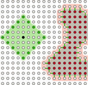
Figure 5: Visualization of the enumeration of $N_{l}$ as in Appendix C. As before, oscillators belonging to the distinguished (shaded) region $I$ are marked , the outside ones are shown as . $\partial O$ is shown as the orange shaded area. $M_{4}(\boldsymbol{i})=\{\boldsymbol{j}\in C|d(\boldsymbol{i},\boldsymbol{j})\leq 4\}$ for a certain oscillator  is shaded green, its surface oscillators $m_{4}(\boldsymbol{i})=\{\boldsymbol{j}\in C|d(\boldsymbol{i},\boldsymbol{j})=4\}$ are depicted by  .

We start by identifying the set of oscillators that can contribute to $N_{l}$, $l>1$,

$$N_{l}=\sum_{\boldsymbol{j}\in O}\sum_{\begin{subarray}{c}\boldsymbol{i}\in I\\ d(\boldsymbol{i},\boldsymbol{j})=l\end{subarray}}1.$$

Oscillators $\boldsymbol{j}\in O$ can only contribute if their distance to the boundary $\partial O$ is not larger than $l-1$,

$$\partial O=\left\{\boldsymbol{j}\in O\;|\;\exists\boldsymbol{i}\in I:d(\boldsymbol{i},\boldsymbol{j})=1\right\}.$$

Thus, we can restrict the sum over $O$ to the set $A_{l}$

$$A_{l}=\bigcup_{\boldsymbol{i}\in\partial O}\left\{\boldsymbol{j}\in O\;|\;d(\boldsymbol{i},\boldsymbol{j})\leq l-1\right\},$$

i.e., we can write

$$N_{l}=\sum_{\boldsymbol{o}\in A_{l}}\sum_{\begin{subarray}{c}\boldsymbol{i}\in I\\ d(\boldsymbol{i},\boldsymbol{o})=l\end{subarray}}1\leq\sum_{\boldsymbol{o}\in A_{l}}\sum_{\begin{subarray}{c}\boldsymbol{i}\in C\\ d(\boldsymbol{i},\boldsymbol{o})=l\end{subarray}}1\leq|A_{l}|m_{l},$$

where $m_{l}$ is the number of surface oscillators of a ball with radius $l$ within the metric $d$, i.e., $m_{l}\leq 2(2l+1)^{D-1}$ for $l\geq 1$. Using the fact that $|\partial O|\leq N_{1}=s(I)$, $|A_{l}|$ can now be bounded from above in the following way

$$|A_{l}|\leq|\partial O|M_{l-1}\leq s(I)M_{l-1},$$

where $M_{l}$ is the volume of a ball with radius $l$ within the metric $d$, i.e., $M_{l}\leq(2l+1)^{D}$. To summarize, we have

$$N_{l}\leq 2(2l-1)^{D}(2l+1)^{D-1}s(I)\leq 2(2l)^{2D-1}s(I).$$

References

- (1) S. J. Summers and R. F. Werner, Phys. Lett. A 110, 257 (1985).
- (2) P. Stelmachovic and V. Buzek, Phys. Rev. A 70, 032313 (2004).
- (3) A. Osterloh, L. Amico, G. Falci, and R. Fazio, Nature 416, 608 (2002).
- (4) T. J. Osborne and M. A. Nielsen, Phys. Rev. A 66, 032110 (2002).
- (5) K. Audenaert, J. Eisert, M. B. Plenio, and R. F. Werner, Phys. Rev. A 66, 042327 (2002).
- (6) G. Vidal, J. I. Latorre, E. Rico, and A. Kitaev, Phys. Rev. Lett. 90, 227902 (2003), quant-ph/0211074; J. I. Latorre, E. Rico, and G. Vidal, Quant. Inf. Comp. 4, 048 (2004), quant-ph/0304098.
- (7) B.-Q. Jin and V. E. Korepin, J. Stat. Phys. 116, 79 (2004); A. R. Its, B.-Q. Jin, and V. E. Korepin, J. Phys. A 38, 2975 (2005).
- (8) M. Fannes, B. Haegeman, and M. Mosonyi, J. Math. Phys. 44, 6005 (2003).
- (9) M. B. Plenio, J. Eisert, J. Dreißig, and M. Cramer, Phys. Rev. Lett. 94, 060503 (2005), quant-ph/0405142.
- (10) J. Eisert and M. B. Plenio, Int. J. Quant. Inf. 1, 479 (2003).
- (11) M. B. Plenio and V. Vedral, Contemp. Phys. 39, 431 (1998).
- (12) M. B. Plenio and S. Virmani, quant-ph/0504163.
- (13) J. P. Keating and F. Mezzadri, Phys. Rev. Lett. 94, 050501 (2005); J. P. Keating and F. Mezzadri, Commun. Math. Phys. 252, 543 (2004).
- (14) P. Calabrese and J. Cardy, J. Stat. Mech. 06, 002 (2004), hep-th/0405152.
- (15) M. Hein, J. Eisert, and H. J. Briegel, Phys. Rev. A 69, 062311 (2004).
- (16) J. K. Pachos and M. B. Plenio, Phys. Rev. Lett. 93, 056402 (2004).
- (17) A. Hamma, R. Ionicioiu, and P. Zanardi, Phys. Rev. A 71, 022315 (2005).
- (18) F. Verstraete and J. I. Cirac, cond-mat/0407066.
- (19) M. M. Wolf, F. Verstraete, and J. I. Cirac, Phys. Rev. Lett. 92, 087903 (2004).
- (20) A. Botero and B. Reznik, Phys. Rev. A 70, 052329 (2004); B. Reznik, A. Retzker, and J. Silman, J. Mod. Opt. 51, 833 (2004); B. Reznik, Found. Phys. 33, 167 (2003).
- (21) I. Peschel, J. Stat. Mech. Th. E P12 (2004).
- (22) N. Lambert, C. Emary, and T. Brandes, Phys. Rev. Lett. 92, 073602 (2004).
- (23) W. Dür, L. Hartmann, M. Hein, M. Lewenstein, and H. J. Briegel, Phys. Rev. Lett. 94, 097203 (2005).
- (24) M. M. Wolf, quant-ph/0503219.
- (25) D. Gioev and I. Klich, quant-ph/0504151.
- (26) R. Orus, quant-ph/0501110.
- (27) J. I. Latorre, C. A. Lütken, R. Rico, and G. Vidal, Phys. Rev. A 71, 034301 (2005), quant-ph/0404120.
- (28) C. Callan and F. Wilczek, Phys. Lett. B 333, 55 (1994), hep-th/9401072.
- (29) J. D. Bekenstein, Lett. Nuovo Cim. 4, 737 (1972).
- (30) J. D. Bekenstein, Phys. Rev. D 7, 2333 (1973).
- (31) J. D. Bekenstein, Contemp. Phys. 45, 31 (2004).
- (32) L. Bombelli, R. Koul, J. Lee, and R. Sorkin, Phys. Rev. D 34, 373 (1986).
- (33) M. Srednicki, Phys. Rev. Lett. 71, 66 (1993).
- (34) C. Holzhey, F. Larsen, and F. Wilczek, Nucl. Phys. B 424, 443 (1995), hep-th/9403108.
- (35) T. M. Fiola, J. Preskill, A. Strominger, and S. P. Trivedi, Phys. Rev. D 50, 3987 (1994).
- (36) J. Cardy and I. Peschel, Nucl. Phys. B 300, 377 (1988).
- (37) K. Zyczkowski, P. Horodecki, A. Sanpera, and M. Lewenstein, Phys. Rev. A 58, 883 (1998); J. Eisert and M. B. Plenio, J. Mod. Opt. 46, 145 (1999); J. Eisert (PhD thesis, Potsdam, February 2001); G. Vidal and R. F. Werner, Phys. Rev. A 65, 032314 (2002); K. Audenaert, M. B. Plenio, and J. Eisert, Phys. Rev. Lett. 90, 027901 (2003); M. B. Plenio, quant-ph/0505071.
- (38) J. Eisert, C. Simon, and M. B. Plenio, J. Phys. A 35, 3911 (2002).
- (39) R. A. Horn and C. R. Johnson, Matrix Analysis (Cambridge University Press, Cambridge, 1985).
- (40) I. Devetak and A. Winter, Proc. R. Soc. Lond. A 461, 207 (2005).
- (41) M. Benzi and G. H. Golub, BIT Numerical Mathematics 39, 417 (1999).
-
(42)
Note that the above choice of does
not restrict
generality: clearly, there exists a diagonal matrix , the elements of which are , such that
and . Hence, there exists a local symplectic transformation relating the Hamiltonian with to the one with . - (43) A. Wehrl, Rev. Mod. Phys. 50, 221 (1978).
- (44) D.J.E. Callaway, Phys. Rev. E 53 3738 (1996).